doi:10.1016/j.astropartphys.2003.09.003

Sensitivity of the IceCube detector to astrophysical sources

of high energy muon neutrinos

J. Ahrens

, J.N. Bahcall

, X. Bai

, R.C. Bay

, T. Becka

, K.-H. Becker

D. Berley

, E. Bernardini

, D. Bertrand

, D.Z. Besson

, A. Biron

E. Blaufuss

, D.J. Boersma

,S.B

€

oser

, C. Bohm

, O. Botner

, A. Bouchta

O. Bouhali

, T. Burgess

, W. Carithers

, T. Castermans

, J. Cavin

W. Chinowsky

, D. Chirkin

, B. Collin

, J. Conrad

, J. Cooley

D.F. Cowen

o,q

, A. Davour

, C. De Clercq

, T. DeYoung

, P. Desiati

R. Ehrlich

, R.W. Ellsworth

, P.A. Evenson

, A.R. Fazely

, T. Feser

T.K. Gaisser

, J. Gallagher

, R. Ganugapati

, H. Geenen

, A. Goldschmidt

J.A. Goodman

, R.M. Gunasingha

, A. Hallgren

, F. Halzen

, K. Hanson

R. Hardtke

, T. Hauschildt

, D. Hays

, K. Helbing

, M. Hellwig

P. Herquet

, G.C. Hill

, D. Hubert

, B. Hughey

, P.O. Hulth

, K. Hultqvist

S. Hundertmark

, J. Jacobsen

, G.S. Japaridze

, A. Jones

, A. Karle

H. Kawai

, M. Kestel

, N. Kitamura

, R. Koch

,L.K

€

opke

, M. Kowalski

J.I. Lamoureux

, H. Leich

, M. Leuthold

, I. Liubarsky

, J. Madsen

H.S. Matis

, C.P. McParland

, T. Messarius

,P.M

esz

aros

o,q

, Y. Minaeva

R.H. Minor

, P. Mio

cinovi

, H. Miyamoto

, R. Morse

, R. Nahnhauer

T. Neunh

€

offer

, P. Niessen

, D.R. Nygren

,H.

€

Ogelman

, Ph. Olbrechts

S. Patton

, R. Paulos

,C.P

erez de los Heros

, A.C. Pohl

, J. Pretz

P.B. Price

, G.T. Przybylski

, K. Rawlins

, S. Razzaque

, E. Resconi

W. Rhode

, M. Ribordy

, S. Richter

, H.-G. Sander

, K. Schinarakis

S. Schlenstedt

, T. Schmidt

, D. Schneider

, R. Schwarz

, D. Seckel

A.J. Smith

, M. Solarz

, G.M. Spiczak

, C. Spiering

, M. Stamatikos

T. Stanev

, D. Steele

, P. Steffen

, T. Stezelberger

, R.G. Stokstad

K.-H. Sulanke

, G.W. Sullivan

, T.J. Sumner

, I. Taboada

, S. Tilav

N. van Eijndhoven

, W. Wagner

, C. Walck

, R.-R. Wang

, C.H. Wiebusch

C.Wiedemann

,R.Wischnewski

,H.Wissing

,K.Woschnagg

,S.Yoshida

Corresponding author. Tel.: +49-33762-77512; fax: +49-33762-77330.

E-mail address:

hwissing@ifh.de(H. Wissing).

0927-6505/$ - see front matter

doi:10.1016/j.astropartphys.2003.09.003

Astroparticle Physics 20 (2004) 507–532

www.elsevier.com/locate/astropart

Institute of Physics, University of Mainz, Staudinger Weg 7, D-55099 Mainz, Germany

Institute for Advanced Study, Princeton, NJ 08540, USA

Bartol Research Institute, University of Delaware, Newark, DE 19716, USA

Department of Physics, University of California, Berkeley, CA 94720, USA

Fachbereich 8 Physik, BUGH Wuppertal, D-42097 Wuppertal, Germany

Department of Physics, University of Maryland, College Park, MD 20742, USA

DESY-Zeuthen, D-15738 Zeuthen, Germany

Universit

Libre de Bruxelles, Science Faculty CP230, Boulevard du Triomphe, B-1050 Brussels, Belgium

Deparment of Physics and Astronomy, University of Kansas, Lawrence, KS 66045, USA

Department of Physics, Stockholm University, SE-10691 Stockholm, Sweden

Division of High Energy Physics, Uppsala University, S-75121 Uppsala, Sweden

Lawrence Berkeley National Laboratory, Berkeley, CA 94720, USA

University of Mons-Hainaut, 7000 Mons, Belgium

SSEC, University of Wisconsin, Madison, WI 53706, USA

Department of Physics, Pennsylvania State University, University Park, PA 16802, USA

Department of Physics, University of Wisconsin, Madison, WI 53706, USA

Department of Astronomy and Astrophysics, Pennsylvania State University, University Park, PA 16802, USA

Vrije Universiteit Brussel, Dienst ELEM, B-1050 Brussels, Belgium

Department of Physics, George Mason University, Fairfax, VA 22030, USA

Department of Physics, Southern University, Baton Rouge, LA 70813, USA

Department of Astronomy, University of Wisconsin, Madison, WI 53706, USA

CTSPS, Clark-Atlanta University, Atlanta, GA 30314, USA

Department of Physics, Chiba University, Chiba 263-8522, Japan

Blackett Laboratory, Imperial College, London SW7 2BW, UK

Department of Physics, University of Wisconsin, River Falls, WI 54022, USA

Departamento de F

ısica, Universidad Sim

n Bol

ıvar, Caracas, 1080, Venezuela

Faculty of Physics and Astronomy, Utrecht University, NL-3584 CC Utrecht, The Netherlands

Received 6 June 2003; received in revised form 27 August 2003; accepted 15 September 2003

Abstract

We present results of a Monte Carlo study of the sensitivity of the planned IceCube detector to predicted fluxes of

muon neutrinos at TeV to PeV energies. A complete simulation of the detector and data analysis is used to study the

detector

s capability to search for muon neutrinos from potential sources such as active galaxies and gamma-ray bursts

(GRBs). We study the effective area and the angular resolution of the detector as a function of muon energy and angle

of incidence. We present detailed calculations of the sensitivity of the detector to both diffuse and pointlike neutrino

fluxes, including an assessment of the sensitivity to neutrinos detected in coincidence with GRB observations. After

three years of data taking, IceCube will be able to detect a point-source flux of

GeV

at a 5

significance, or, in the absence of a signal, place a 90% c.l. limit at a level of

GeV. A diffuse

flux would be detectable at a minimum strength of

GeV.

A GRB model following the formulation of Waxman and Bahcall would result in a 5

effect after the observation of 200

bursts in coincidence with satellite observations of the gamma rays.

PACS:

95.55.Vj; 95.85.Ry

Keywords:

Neutrino telescope

; Neutrino astronomy; IceCube

1. Introduction

The emerging field of high-energy neutrino

astronomy [1–3] has seen the construction, opera-

tion and results from the first detectors, and pro-

posals for the next generation of such instruments.

The pioneering efforts of the DUMAND [4]

collaboration were followed by the successful

508

J. Ahrens et al. / Astroparticle Physics 20 (2004) 507–532

deployments of NT-200 at Lake Baikal [5] and

AMANDA [6] at the South Pole. These detectors

have demonstrated the feasibility of large neutrino

telescopes in open media like sea- or lake-water and

glacial ice. They have been used to observe neu-

trinos produced in the atmosphere [7] and to set

limits on the flux of extraterrestrial neutrinos [8,9]

which are significantly below those obtained from

the much smaller underground neutrino detectors

[10,46]. The results obtained so far, together with

refinements of astrophysical theories predicting

extraterrestrial neutrino fluxes from cosmic sour-

ces, have provided the impetus to construct a

neutrino observatory on a much larger scale. Pro-

posals for a detector in the deep water of the

Mediterranean have come from the ANTARES

[11], NESTOR [12] and NEMO [13] collabora-

tions. IceCube is a projected cubic-kilometer

under-ice neutrino detector [14–16], to be located

near the geographic South Pole in Antarctica.

The IceCube detector will consist of optical

sensors deployed at depth into the thick polar ice

sheet. The ice will serve as Cherenkov medium for

secondary particles produced in neutrino interac-

tions in or around the instrumented volume. The

successful deployment and operation of the

AMANDA detector have shown that the polar ice

is a suitable medium for a large neutrino telescope

and the analysis of AMANDA data has proven

the science potential of such a detector.

IceCube will offer great advantages over

AMANDA beyond its larger size: it will have a

higher efficiency and a higher angular resolution in

reconstructing muon tracks, it will map electro-

magnetic and hadronic showers (

cascades

) from

electron- and tau-neutrino interactions and, most

importantly, it will have a superior energy resolu-

tion. Simulations, backed by AMANDA data,

indicate that the direction of muons can be deter-

mined with subdegree accuracy and their energy

measured to better than 30% in the logarithm of

the energy. For electron neutrinos that produce

electromagnetic cascades, the direction can be

reconstructed to better than 25

and the response

in energy is linear with a resolution better than

10% in the logarithm of the energy [16]. Good

energy resolution is crucial in that it allows full

sky coverage for ultrahigh-energy extraterrestrial

neutrinos, since no atmospheric muon or neutrino

background exceeds 1 PeV in a deep, cubic-kilo-

meter detector.

IceCube will be able to investigate a large

variety of scientific questions in astronomy, astro-

physics, cosmology and particle physics [16,22]. In

this paper we focus on the IceCube performance in

searching for TeV to PeV muon neutrinos, as ex-

pected from sources such as active galactic nuclei

(AGN), gamma-ray bursts (GRBs) or other cos-

mic accelerators observed as TeV gamma-ray

emitters. We present the results of a Monte Carlo

study that includes the simulation of the detec-

tor and the full analysis chain, from filtering of

the triggered data to event reconstruction and

selection. We assess basic detector parameters,

such as the pointing resolution and the effective

area of the detector, directly from simulated data.

We also present a detailed calculation of the de-

tector

s sensitivity to both diffuse and pointlike

neutrino emission following generic energy spec-

tra, providing benchmark sensitivities for some of

the fundamental goals in high-energy neutrino

astronomy.

2. The IceCube detector

The IceCube detector is planned as a cubic-

kilometer-sized successor to the AMANDA detec-

tor. It will consist of 4800 photomultiplier tubes

(PMTs) of 10-inch diameter, each enclosed in a

transparent pressure sphere. These optical modules

(OMs) will be arrayed on 80 cables, each such

string

comprising 60 modules spaced by 17 m. During

deployment the strings will be lowered into vertical,

water-filled holes, drilled to a depth of 2400 m with

pressurized hot water, and allowed to freeze in

place. The instrumented volume will span a depth

from 1400 to 2400 m below the ice surface. In the

horizontal plane the strings will be arranged in a

triangular pattern such that the distances between

each string and its up-to-six nearest neighbors are

125 m (Fig. 1). This configuration is the result of an

extensive optimization procedure [18,19].

The relatively sparse instrumentation is made

possible by the low light absorption of the deep

Antarctic ice. The absorption length for light from

J. Ahrens et al. / Astroparticle Physics 20 (2004) 507–532

509

UV to blue varies between 50 and 150 m, depend-

ing on depth. Light scattering, on the other hand,

will result in strong dispersion of the Cherenkov

signal over large distances, diluting the timing

information carried by the photons. This scatter-

ing effect increases with the average distance at

which photons are collected, but is somewhat com-

pensated for by the information contained in the

time structure of the recorded PMTpulse, since,

e.g., its length is a measure for the distance to the

point of light emission.

As a significant improvement over the

AMANDA technology, each IceCube OM will

house electronics to digitize the PMTpulses, so

that the full waveform information is retained [17].

The waveforms will be recorded at a frequency of

about 300 mega-samples per second, leading to an

intrinsic timing accuracy for a single pulse mea-

surement of 7 ns. The digitized signals will be

transmitted to the data acquisition system, located

at the surface, via twisted-pair cables. Each OM

will communicate, through an embedded CPU,

with its nearest neighbors by means of a dedicated

copper-wire pair. This enables the implementation

of a local hardware trigger in the ice, such that

digitization occurs only when some coincidence

requirement has been met [16]. This is particularly

important in order to suppress the transmission of

pure noise pulses, which, unlike photon pulses

from high-energy particles, are primarily isolated,

i.e., occur without correlation to pulses recorded in

neighboring and nearby OMs. (The dark noise rate

of an OM will be as low as 300–500 Hz, due to the

sterile and low-temperature environment.) Local

triggers will be combined by surface processors to

form a global trigger. Triggered events will be fil-

tered and reconstructed on-line, and the relevant

information will be transmitted via satellite to re-

search institutions in the northern hemisphere.

The complete detector will be operational per-

haps as soon as five years after the start of con-

struction, but during the construction phase all

deployed strings will already produce high-quality

data.

AMANDAII

SPASE2

Old Pole Station line

Runway

South

Pole

Dome

125 m

north

Grid

Fig. 1. Schematic view of the planned arrangement of strings of the IceCube detector at the South Pole station. The existing

AMANDA-II detector will be embedded in the new telescope, and the SPASE-2 air-shower array will lie within its horizontal

boundaries.

510

J. Ahrens et al. / Astroparticle Physics 20 (2004) 507–532

The IceCube array deep in the ice will be

complemented by IceTop, a surface air-shower

array consisting of 160 frozen-water tanks. The

tanks will be arranged in pairs, separated by a few

meters, one on top of each IceCube string. IceTop

is the logical extension of the SPASE surface array

[20] which already is a unique asset for AMA-

NDA. The air-shower parameters measured at the

surface combined with the signal from the high-

energy muon component at depth provide a new

measure for the primary composition of cosmic

rays. Furthermore, data from IceTop will serve as

a veto for air-shower-induced background and will

enable cross-checks for the detector geometry

calibration, absolute pointing accuracy and angu-

lar resolution. In addition, the energy deposited by

tagged muon bundles in air-shower cores will be

an external source for energy calibration.

3. Simulation and analysis chain

The science potential of a kilometer-scale neu-

trino telescope has been assessed in previous papers

by convoluting the expected neutrino-induced

muon flux from various astrophysical sources with

an assumed square-kilometer effective detector

area [21–23]. In this work we use a full simulation

of event triggering, reconstruction and data selec-

tion to assess the detector capabilities. The simu-

lation of the detector response and the analysis of

Monte Carlo-generated data rely on software

packages presently provided by the AMANDA

collaboration [24,40]. This means that the software

concepts and analysis techniques used here have

proven capable and have been verified by real data

taken with the AMANDA detector. However, a

full simulation of the IceCube hardware was not

possible with the present software. The simulated

data correspond to the original AMANDA read-

out, which does not yield full waveforms for the

PMTpulses, but only leading-edge times and peak

amplitudes (of which only the timing information

is used in the reconstruction). More advanced

analysis methods which take advantage of the

additional information were not applied and hence

this work may yield a conservative assessment of

the IceCube performance.

3.1. Event generation

The backgrounds for searches for extrater-

restrial neutrinos come from the decay of mesons

produced from cosmic-ray interactions in the

atmosphere. The decay products include both

muons and neutrinos. The muons created above

the detector will be responsible for the vast

majority of triggers, since they are sufficiently

penetrating to be capable of reaching the detector

depth. Air-shower-induced events can be identi-

fied by the fact that they involve exclusively

downward tracks and a comparatively small de-

posit of Cherenkov light in the detector, as the

muons will have lost most of their energy upon

reaching the detector. However, an upward track

might be faked if two uncorrelated air showers

produce time-coincident muons within the detec-

tor. About three percent of all triggered events

will be caused by muons from two independent

air showers.

The simulation packages

Basiev

[25] and

Corsika

[26] were used to generate cosmic-ray-

induced muon background. Roughly 2.4 million

events containing muon tracks from one single air

shower (

Atm

single

) were simulated with primary

energies up to 10

GeV. High-energy events and

events containing tracks close to the horizon were

oversampled, in order to achieve larger statistics at

high analysis levels. In addition, we simulated one

million events containing tracks from two inde-

pendent air showers (

Atm

double

Muons induced by atmospheric neutrinos

(

Atm

) form a background over the full sky and

up to very high energies. However, the energy

spectrum of atmospheric neutrinos falls steeply

like d

, whereas one expects an

energy spectrum as hard as

from shock-

acceleration mechanisms in anticipated cosmic

TeV-neutrino sources. Therefore, cosmic-neutrino

energies should extend to higher values and cause

more light in the detector than will atmospheric

neutrinos. The amount of light observed in an

event is therefore useful as a criterion to separate

high-energy muons induced by cosmic neutrinos

from those induced by atmospheric neutrinos. An

uncertainty in the flux of atmospheric neutrinos

at high energies arises from the poorly known

J. Ahrens et al. / Astroparticle Physics 20 (2004) 507–532

511

contribution from prompt decays of charmed

mesons produced in the atmosphere. The prompt-

charm-related muon-neutrino fluxes predicted by

various theoretical models [27,28] show large

variations. Most of the uncertainty is associated

with the extrapolation of charm-production mod-

els to high energies. Models applying perturbative

QCD, for example, predict higher fluxes than non-

perturbative QCD approaches.

Neutrino-induced events were simulated with

the program

nusim

[29], which allows the gener-

ation of muon neutrinos with arbitrary energy

spectra. Neutrinos are sampled from an

spec-

trum and are then reweighted to produce user-

defined energy spectra, as required. The code

includes a simulation of neutrino propagation

through the Earth, taking into account absorption

in charged-current interactions as well as neutral-

current regeneration. The neutrino cross sections

are calculated using the MRSG [30] parton distri-

butions. The column density of nucleons to be

traversed is calculated according to the Preliminary

Reference Earth Model [31]. Muons that are

produced in the rock beneath the detector are

propagated to the rock/ice boundary using the

Lipari–Stanev [32] muon propagation code. In to-

tal, we simulated 7.4

events induced by neu-

trinos with primary energies up to 10

GeV. The

flatness of the generated

neutrino spectrum

leads to a statistically beneficial oversampling of

events at high energies for the mostly softer energy

spectra investigated.

For the ‘‘conventional’’ flux of atmospheric

neutrinos (i.e., the component related to decays of

pions and kaons) we apply the prediction calcu-

lated by Lipari [33]. For the prompt-charm con-

tribution we compare the predictions from two

different charm-production models: a phenome-

nological non-perturbative approach, the Recom-

bination Quark Parton Model (

rqpm

), by Bugaev

et al. [34], and perturbative QCD calculations

made by Thunman et al. (

TIG

) [35]. The prompt-

neutrino event rate predicted by

TIG

is the lower

by more than an order of magnitude, and is low

even when compared to other calculations using

non-perturbative QCD (e.g., [36]), and may

therefore serve as a lower limit for the prompt-

charm contribution.

For the flux of extraterrestrial neutrinos (

Cos-

mic

) we apply a generic

energy spectrum, as

expected from shock acceleration. We use a source

strength of

GeV as a benchmark diffuse flux of extraterres-

trial neutrinos. This is the logarithmic mean of two

upper bounds on the diffuse neutrino flux: (a) the

bound obtained if one assumes that the neutrino

sources are completely transparent to neutrons

and that these sources are responsible for the ob-

served flux of ultrahigh-energy cosmic rays, while

one does not allow for cosmological evolution of

the sources, and (b) the bound obtained if one

assumes that the sources are opaque to neutrons

and only high-energy gamma rays escape ([2] and

references therein). The flux is an order of mag-

nitude below present experimental limits set on the

flux of muon neutrinos [9] and electron neutrinos

[37].

3.2. Muon propagation

The propagation of muons through the ice is

modeled with either the code by Lohmann et al.

[38] (for muon energies smaller than 10

GeV) or

the code by Lipari and Stanev [32] (for muon

energies greater than 10

GeV). These codes cal-

culate the stochastic-radiative and nuclear-inter-

active energy losses along the muon track within

or close to the instrumented detector volume.

The complete tracking of all Cherenkov pho-

tons produced by the muon and associated

stochastic-radiative energy losses for each event

would require an impractical amount of comput-

ing power. Therefore, the photon amplitudes and

timing distributions at all points in space from

both a muon and an electromagnetic cascade are

pre-calculated and tabulated for fast lookup using

the

PTD

[39] software package. This simulation

takes into account the scattering and absorption

properties of the ice as well as the response of

the PMT.

3.3. Detector simulation

The response of the entire array of optical

modules is modeled with the detector simulation

512

J. Ahrens et al. / Astroparticle Physics 20 (2004) 507–532

amasim

[40,41]. The actual number of photons at

an OM is found by sampling from a Poisson dis-

tribution with a mean amplitude computed by

summing over all contributing muons and cascades.

The arrival times of these photons are sampled

from the pre-tabulated distributions. Noise pulses

are added assuming a PMTnoise rate of 500 Hz.

For event triggering, and to suppress PMTnoise,

we require at least five local coincidences in a

global trigger time window of 7

s. A local coin-

cidence is defined as the registration of at least two

pulses within 1

s among an OM and its nearest

and next-to-nearest neighbors. Only pulses that

are part of a local coincidence are read out and

used for further reconstruction.

The detector geometry used in this simulation

differs from the finalized design in the total num-

ber of strings (we have simulated a detector with

75 strings instead of 80), the total number of OMs

(4575 instead of 4800), the instrumented string

length (960 m instead of 1000 m) and the depth of

the detector center (which was simulated at 2000

m, while it will lie at 1900 m in the updated de-

sign). The spatial arrangement with the strings

spaced 125 m apart on a triangular grid is in

accordance with the design presented in the pre-

vious section. A simulation of the detector in its

finalized configuration using a subsample of the

Monte Carlo-generated events showed an increase

in the expected event rates of roughly 10% for both

signal and background at trigger level.

3.4. Event reconstruction

The reconstruction of an event involves fitting a

muon track hypothesis to the recorded pattern of

PMTpulses (‘‘hits’’) assumed to be caused by

Cherenkov photons generated by the muon.

Triggered events are first reconstructed with three

fast ‘‘first guess’’ algorithms which use the arrival

times of the photons or the topology of OMs

having registered a hit: (1) The

line fit

(LF) is based

on a simple analytic

minimization [42]. It fits the

free parameters (vertex position and velocity) of a

hypothetical straight-line trajectory to the one-

dimensional projection of the observed pattern of

hits. (2) The

dipole approximation

[43] is based on

the hit topology. The sum of all unit vectors

pointing from one hit to the next in time gives a

‘‘dipole vector’’

. The direction of

is corre-

lated to the direction of the incoming track(s),

while its absolute value is a measure of the good-

ness of the approximation. (3) The

direct walk

algorithm

(DW) [43] posits as track hypotheses the

straight-line connections between every pair of hits

that have occurred in separate OMs with a time

difference consistent with the muon flight time

between these two OMs. Those track hypotheses

that pass a consistency check with respect to the

complete hit pattern of the event are combined to

obtain an estimate of the track parameters.

Following these first-guess methods, the events

are reconstructed using a full

maximum likelihood

reconstruction

(LR) [43,44]. The probabilities in

the likelihood function are based on the arrival-

time distribution of photons emitted along a track

as a function of distance and angle of the track

with respect to the OM. These distributions have

been obtained from a detailed photon-propagation

simulation. The reconstruction used here relies

only on the timing information carried by the

first

photon that is recorded by the OM. This corre-

sponds to the current practice in AMANDA,

whose original read-out only yields minimal timing

information for the pulses (leading and trailing

edges at the corresponding threshold crossings)

and the peak amplitude seen by the PMTin the

event.

4. Basic performance capabilities

The trigger rate for a fivefold local coincidence

trigger was found to be 1.7 kHz. This includes

a 50 Hz rate of triggers due to uncorrelated

time-coincident air showers (

Atm

double

). As

described below, a set of event selection criteria

In contrast, the IceCube electronics will retain the full pulse

shape. Detailed hit information can then be extracted from the

integrated charge and the peak structure of the pulse. Future

reconstructions will therefore profit from the additional infor-

mation carried by consecutively arriving photons which were

multiple-scattered and delayed on their way from the muon

track to the PMT.

J. Ahrens et al. / Astroparticle Physics 20 (2004) 507–532

513

was established that removes the bulk of the

downward cosmic-ray-induced muons, but still

yields a high passing rate for upward muons from

atmospheric neutrinos. These atmospheric-neu-

trino events would then form the main back-

ground in searches for cosmic neutrinos. We use

this level of data reduction as a baseline perfor-

mance measure.

4.1. Event selection

The most effective handle to reject the back-

ground of downward cosmic-ray-induced muons is

provided by the zenith angles

obtained from the

various reconstruction and filter algorithms (

and

). The most straightforward way

to reject cosmic-ray muons would be to exclusively

select upward tracks. However, muons from PeV

or EeV neutrino interactions are expected to arrive

from directions close to or above the horizon, so it

is worthwhile to combine the angular cut with an

energy criterion. If the neutrino interaction occurs

close to the detector, the energy deposit of the

daughter muon will be large enough to distinguish

it from low-energy cosmic-ray muons. An estima-

tor of this energy deposit is the number of OMs (or

‘‘channels’’) that have registered a hit. We there-

fore accept downward tracks provided the channel

multiplicity,

, of the event is sufficiently large.

The selection criteria used in the data reduction

are listed in Table 1. The first three criteria are

based on the estimates of track directions obtained

from the three first-guess methods and aim at the

early rejection of low-energy downward cosmic-

ray muons. The level of data reduction achieved

with the application of cuts 1–3 will be referred to

as ‘‘level 1’’.

The higher ‘‘level 2’’, defined by cuts 4–9, is

based on variables from the more accurate (and

more CPU intensive) LR:

•

Events reconstructed with zenith angles smaller

than 85

(i.e., directions more than 5

above the

horizon) are rejected, as long as

is less than

150. The

criterion is tightened with decreas-

ing zenith angle

[cut 4].

Apart from the direction criterion, the LR

provides a series of quality parameters, which we

apply cuts on in order to select a sample of high-

quality and well-reconstructed events:

•

We require the

reduced likelihood

to be suf-

ficiently small.

is given by the negative loga-

rithm of the likelihood of the best-fit track

hypothesis divided by the number of degrees

of freedom of the fit, hence a

small

value indi-

cates a good track quality [cut 5].

•

We require a minimum

number of direct hits

direct

, i.e., hits that have occurred with a rela-

tively short delay (<150 ns) relative to the arrival

time predicted for an unscattered Cherenkov

photon emitted from the reconstructed track

[cut 6].

•

We require a minimum

track length

, i.e., a

minimum distance along the reconstructed track

over which the hits were detected. We define this

length as the maximum distance between two hit

positions projected on the straight line defining

the track direction. A more stringent criterion

is a lower bound on the track length based only

on direct hits

direct

[cut 7].

•

The consistency of the fitted track direction is

checked with the

smoothness parameter

[7,43].

It is a measure of the evenness of the projection

of the hit positions along the track, based on

a Kolmogorov–Smirnov test. The smoothness

parameter is calculated both with all hits

and exclusively with direct hits

direct

[cut 8].

•

For high-quality tracks, the various reconstruc-

tion methods are likely to produce similar

results close to the true track direction. We

therefore require the difference in zenith angles

obtained by two different methods to be small

[cuts 9 and 3].

These quality criteria are particularly important

for muons that travel merely a short distance

through the instrumented detection volume, e.g.,

The detector coordinate system is oriented such that a

zenith angle of

corresponds to vertically downward-

going tracks, and, correspondingly, tracks from straight below

the detector have

180

514

J. Ahrens et al. / Astroparticle Physics 20 (2004) 507–532

low-energy muons or muons that pass only

through the rim of the detector or even outside its

geometrical volume. These muons will cause hits in

fewer OMs and therefore provide less information

for the reconstruction. Most of the quality criteria

are therefore tightened if

is small.

4.2. Muon detection rates

We compare the detector response as well as the

event selection efficiency for all types of events:

cosmic-ray muons, muons induced by atmospheric

neutrinos and muons from cosmic neutrinos

with a hard energy spectrum, following an

power law. The numbers of triggered and selected

events at each level, normalized to one year of data

taking, are listed in Table 2. With a flux of

GeV adopted as a

benchmark for the flux of cosmic neutrinos, we

expect more than 1000 signal events per year at

level 2. At this level, both the background from

atmospheric neutrinos and the background from

cosmic-ray muons yield roughly 10

events per

year. The

rqpm

model for atmospheric charm

predicts a contribution of almost 5000 prompt-

charm events to the atmospheric background. The

TIG

model predicts thirty times fewer events.

Fig. 2 shows distributions of the reconstructed

zenith angle,

, for the four event classes

(

Cosmic

Atm

single

and

Atm

double

)at

different cut levels. The level 1 selection removes

the bulk of low-energy downward cosmic-ray-

induced background. The cuts on the zenith angles

from the first-guess methods being relatively soft,

most of the remaining background is located in the

angular region around 30

above the horizon

Table 1

Definitions of individual cuts and cut levels

Parameter Cut Explanation

Level 1

50 Zenith-angle criterion based on LF, applied for low-multiplicity

events

2 Zenith-angle criterion based on

, applied for high goodness-of-

fit values

Consistency of LF and DW

Level 2

>85

150

250

cos

Zenith-angle criterion of LR which is weakened with increasing

channel multiplicity

<10 Reduced likelihood of LR

direct

>10 if

50 Requirement of 10 direct hits for low-multiplicity events

>300 m

and

Requirement of minimum track length, using direct hits for

multiplicities smaller than 150

direct

>300 m if

150

<0.5

and

Constancy of light output along the track, requirement is

tightened for low multiplicities

direct

<0.5 if

<10

150 Consistency of LF and LR

Cut level 1 uses the ‘‘first-guess’’ zenith angles

and

as obtained from the

linefit

, the

dipole approximation

and the DW

algorithm. Level 2 exploits the fitted zenith angle from the

, and various quality parameters from the fit, such as the reduced

likelihood

, the number of unscattered photons

direct

, the track length

(

direct

) defined as the maximum distance between the

positions of two (direct) hits projected on the track, the

smoothness

parameters

and

direct

which are a measure of the evenness of the

light emission along the track and the difference between the zenith angles

and

. Most of the cuts are varied with the number of

modules (or channels),

, that have recorded at least one hit in the event. A zenith angle of

corresponds to a vertically

downward-going track.

J. Ahrens et al. / Astroparticle Physics 20 (2004) 507–532

515

cos

. Level 2 then restricts the allowed

zenith region to less than 5

above the horizon,

except for very bright (i.e., high-multiplicity)

events. The remaining ordinary cosmic-ray muon

background (

Atm

single

) at level 2 is concentrated

at the horizon and could be rejected with a tight-

ened cut on the zenith angle, while the sample of

cosmic-ray-induced background composed of

muons from two air showers (

Atm

double

) still

contains misreconstructed events that ‘‘fake’’ an

upward-going track. However, level 2 does not

contain a definite energy discrimination, required

to separate the high-energy signal of cosmic neu-

trinos from the atmospheric-neutrino background.

In the simplest approach this energy selection is

accomplished by an additional tight cut on the

channel multiplicity. This final cut, which has to be

optimized for different analysis purposes (see Sec-

tion 5.2), will lead to a drastic reduction of all

three classes of background. In this analysis, none

of the cosmic-ray muon events passed this addi-

tional

cut.

Simulated energy spectra for muons generated

by cosmic and atmospheric neutrinos are shown in

Fig. 3. At the point of their closest approach to the

detector center, muons from a cosmic

neutrino

source typically have energies in the TeV–PeV

range, whereas the energy distribution for the

background of muons induced by atmospheric

neutrinos peaks between 100 and 300 GeV. Fig. 4

shows channel-multiplicity distributions at level 2

for all event classes. The signal class of high-energy

cosmic neutrinos shows a clear excess at high

multiplicities compared to the lower-energy back-

ground classes.

4.3. Effective detector area

As a measure of the detector efficiency we use

the effective detector area, defined as

eff

;

Þ¼

detected

;

generated

;

gen

;

where

detected

is the number of events that trigger

the detector or pass the cut level under consider-

ation, from a test sample of

generated

muons that

have an energy

at a given point within the

fiducial volume and an incident zenith angle

.In

the following, we give

at the point of closest

approach to the detector center (which might lie

outside the geometrical detector volume). The

fraction of generated to triggered or selected

events is scaled with the size of the generation

plane,

gen

, which is the cross-sectional area of the

cylinder that contains all generated muon tracks

with directions parallel to its axis.

The effective area will depend on the muon

energy, since very bright high-energy muons will

trigger the detector and pass the selection criteria

more efficiently. It will also depend strongly on the

zenith angle of the incident muon after event

selection, since low-energy muons are always re-

Table 2

Passing rates

for signal and background events predicted for one year of data

Trigger Level 1 Level 2

Cosmic

3331 ± 6 2172 ± 4 1089 ± 3

Atm

(824 ± 4)

(264 ± 2)

(91 ± 1)

TIG

(0.97 ± 0.003)

(0.40 ± 0.002)

(0.17 ± 0.001)

[0.1%] [0.2%] [0.2%]

rqpm

(24.8 ± 0.07)

(11.08 ± 0.04)

(4.85 ± 0.03)

[3%] [4%] [5%]

Atm

single

(5.2 ± 0.01)

(1.3 ± 0.01)

(72 ± 3)

Atm

double

(1.6 ± 0.02)

(4.6 ± 0.3)

(28 ± 7)

The signal expectation corresponds to a source flux of

GeV. The expectation for atmospheric-

neutrino events is listed separately for the ‘‘conventional’’ component and the ‘‘prompt’’ component (following [35] (

TIG

) and [34]

(

rqpm

)). The fraction of prompt-charm events with respect to the whole atmospheric-neutrino sample is given in square brackets. The

numbers of cosmic-ray muon background events are shown separately for events that contain muon(s) from only one air shower (

Atm

single

) and those that contain muons from two accidentally coinciding air showers (

Atm

double

). The quoted uncertainties are statistical

only.

516

J. Ahrens et al. / Astroparticle Physics 20 (2004) 507–532

jected if they arrive from above the horizon. Thus,

the effective area for a neutrino telescope, as it is

defined here, is a priori zero for downward events

below a certain energy.

In order to expose only the

energy

dependence

of the trigger- and selection efficiencies, we have

computed

eff

using a sample of muons which

arrive from below the horizon, i.e., tracks with

incident zenith angles larger than 90

(or cos

0). This has the advantage that the angular cuts,

which reject low-multiplicity downward muons,

have no impact on the signal (except for com-

pletely misreconstructed events) and so the effi-

ciency is not artificially reduced by the ‘‘blindness’’

of the experiment to low-energy muons from the

southern sky. Fig. 5 shows the effective area as a

function of the muon energy for muons arriving

from the northern sky. At trigger level the detector

shows a sizeable acceptance even for low-energy

events. The effective trigger area reaches one

square kilometer at a few hundred GeV. Sensitiv-

ity to sub-TeV signals is required for science mis-

sions like the search for weakly interacting massive

particles (WIMPs). WIMPs might be trapped in

Trigger

Level 1

Level 2

Trigger

Level 1

Level 2

Trigger

Level 1

Level 2

cos

Events / Year

1 0.8 0.6 0.4 0.2 0 0.2 0.4 0.6 0.

Atm

cos

Events / Year

1 0.8 0.6 0.4 0.2 0 0.2 0.4 0.6 0.

Atm

single

cos

Events / Year

1 0.8 0.6 0.4 0.2 0 0.2 0.4 0.6 0.

Atm

double

cos

Events / Year

1 0.8 0.6 0.4 0.2 0 0.2 0.4 0.6 0.8

Fig. 2.

Reconstructed zenith angle

for signal from a diffuse flux of cosmic neutrinos following an

spectrum of intensity

GeV (top left), atmospheric neutrino background including

rqpm

charm according to [34] (top

right), and atmospheric muon background from single air showers (bottom left) and from two coincident air showers (bottom right).

The individual histograms in each plot correspond to trigger level (solid lines) and after applying level 1 (dashed lines) and level 2

(dotted lines) cuts. Event numbers are normalized to one year. The irregular shapes of the level 2 distributions in the lower plots are due

to the low number of events (before normalization) remaining in the simulated samples at this level.

J. Ahrens et al. / Astroparticle Physics 20 (2004) 507–532

517

the center of the Earth where they can annihilate

pairwise, producing muon neutrinos that can be

detected by IceCube. A dedicated selection, tai-

lored to select vertical, upward-going tracks, could

retain most of the triggered signal in the GeV

range [16].

The search for high-energy extraterrestrial

neutrinos, on the other hand, would benefit from a

raised energy threshold, as the signal-to-back-

ground ratio improves with increased energy. The

optimal threshold, i.e., the threshold that maxi-

mizes the sensitivity to a given signal, is deter-

mined by the shape of the signal energy spectrum.

For instance, a hard signal spectrum like

Trigger

Level 1

Level 2

log

/ GeV)

Events / Year

100

120

140

Atm

log

/ GeV)

Events / Year

10000

20000

30000

40000

50000

60000

70000

0 1 23 4 5 67 8 9 0 1 23 4 5 67 8 9

Fig. 3.

Energy spectra for neutrino-induced muons at different cut levels

for signal from an

source (left) and atmospheric neutrino

background (right). Each plot shows the muon energy at the point of closest approach to the detector center and compares the spectra

at trigger level (solid lines) and after applying level 1 (dashed lines) and level 2 (dotted lines) cuts.

Atm

(rqpm)

Atm

(TIG)

Events / Year

0 100 200 300 400 500 600 700 800

Fig. 4.

Channel multiplicity at level 2

for signal from an

source (dashed), atmospheric neutrinos including the two

alternative charm contributions

TIG

(sparse dots) and

rqpm

(dense dots) and cosmic-ray muon events (solid).

/ GeV)

log

0 1 2 345 6 7 8

]

[km

eff

0.2

0.4

0.6

0.8

1.2

1.4

1.6

1.8

2.2

Trigger

Level 2

> 20

> 30

Fig. 5.

Effective area as a function of the muon energy

at trigger

level, after level 2 selection and after additional energy-sensitive

cuts on the number of channels

that have recorded at least

one hit. The effective area was calculated using a muon sample

with arrival directions from the northern sky only, meaning that

the data points reflect an average over one hemisphere.

518

J. Ahrens et al. / Astroparticle Physics 20 (2004) 507–532

would suggest a tighter cut than a softer

spectrum. After imposing level 2 cuts the detector

still has an effective area of

0.3 km

for upward-

moving muons of a few tens of GeV. Additional

cuts from level 2 on, optimized with respect to

different signal hypotheses, in some cases shift the

threshold considerably to higher energies. Fig. 5

includes the effective area after adding energy-

separation cuts requiring the channel multiplicity

to be larger than 20 and 30 respectively. Such

cuts are applied in the search for high-energy

neutrinos from steady point sources. The tighter

requirement

, for instance, is the result

of an optimization procedure (see Section 5)

assuming a pointlike

signal and an exposure

time of one year. This cut only affects events at

energies below 10 TeV (where most of the atmo-

spheric background lies), while full efficiency is

retained at higher energies. For an

signal

spectrum and the same exposure time, the opti-

mization yields a looser cut,

20, which has

less impact on the energy threshold. (The impact

on the energy threshold resulting from the addi-

tional

cuts optimized for diffuse and pointlike

signals can also be seen in Figs. 13 and 17.

Note, however, that these figures show the energy

spectra of the primary neutrino, rather than the

muon energy at the detector.)

While in Fig. 5 the effective area was averaged

over all directions throughout the northern sky,

Fig. 6 shows the effective area as a function of

zenith angle of the muon track over the full sky,

from vertically upward-going

cos

¼?

vertically downward-going

cos

.Ineach

of the four discrete energy intervals shown sepa-

rately, the effective area reflects an average value

for a sample of muons induced by neutrinos with

an initial energy spectrum proportional to

The detector will have an effective detection area

of one square kilometer for upward-moving muons

in the TeV range. Above 100 TeV the selection

allows the detection of downward neutrinos, i.e.,

an observation of the southern sky

cos

In the PeV range the effective area for downward

muons is at least 0.6 km

, increasing towards the

horizon. This means that for these energies Ice-

Cube can observe a large part of our Galaxy,

including the Galactic center. When seen from the

South Pole, the Galactic center is located approxi-

mately 30

above the horizon, which corresponds

to cos

5 in detector coordinates. In that

direction, the effective area is

0.2 km

at 0.1–

1 PeV, rising to 0.8 km

for PeV muons.

4.4. Angular resolution

The angular resolution for reconstructed muon

tracks is an important quantity in the search for

neutrinos from point sources. A higher angular

resolution allows the use of a smaller search bin,

resulting in a lower background rate per bin and

thus a higher signal-to-noise ratio.

We characterize the reconstruction error by the

angle

between the true and the reconstructed

directions of the simulated muon tracks. Fig. 7

shows the distribution of

at level 2 for the entire

signal sample of muons from neutrinos with an

energy spectrum. The median of this distribution

can be used as a simple measure of the pointing

resolution. It corresponds to the size (i.e., the

opening half-angle) of the angular cone about the

true track direction in which 50% of the recon-

structed tracks lie. The overall median angular

error for the

signal sample is about 0.8

cos

1 0.5 0 0.5 1

]

[km

eff

0.2

0.4

0.6

0.8

1.2

1.4

1100 PeV

100TeV1PeV

1TeV10TeV

100GeV1TeV

Fig. 6.

Effective area at level 2 as a function of the zenith angle.

The effective area was calculated for muons in four separate

energy ranges after imposing level 2 cuts.

J. Ahrens et al. / Astroparticle Physics 20 (2004) 507–532

519

However, the reconstruction accuracy depends

on the energy and angle of incidence of the muon.

The median angular error is shown in Fig. 8 as a

function of the cosine of the zenith angle of the

muon for four different muon energy ranges.

For muon energies from 100 GeV to 1 TeV the

median angular error approaches 1

for tracks

with zenith angles smaller than roughly 140

cos

. For nearly vertical, upward-

going tracks of low-energy muons the angular

resolution is worse, because such events are likely

to cause hits in optical modules on a single string

only. However, the reconstruction accuracy in this

energy range is similar to the mean angle between

the muon and the initial neutrino. In the more

promising higher energy range, a few TeV and

above, the resolution is substantially higher and its

zenith-angle dependency weaker. Most of the sig-

nal in the TeV–PeV range will be reconstructed

with an accuracy significantly better than 1

.The

angular error for muons with energies between 1

and 100 PeV is shown only above cos

15,

i.e., only down to 10

or so below the horizon,

since the Earth becomes opaque to muon neutri-

nos with sufficient energy to induce muons at these

energies. For downward muons, the reconstruc-

tion error is smaller for sub-PeV muons than for

muons in the PeV range. This is due to the angular

selection at level 2 (cut 4 in Table 1) which only

retains events with zenith angles less than 85

they have a large channel multiplicity

. Muons

with TeV energies, compared to the much brighter

PeV muons, have to travel a longer path inside the

instrumented volume in order to fulfill the

requirement, and will thus be reconstructed more

accurately. A significant improvement in the

reconstruction of PeV events is expected with

further development of the reconstruction, in

particular from including amplitude and waveform

information.

Apart from using the median angular error, the

reconstruction resolution can also be characterized

in terms of the width of the two-dimensional dis-

tribution of the angular deviation of reconstructed

track directions from the true track direction. This

so-called ‘‘point-spread function,’’ expressed in

spherical detector coordinates

and

such that

all bins span equal solid angles, is shown in Fig. 9.

This two-dimensional function being fairly

symmetric, we calculate the density of recon-

structed tracks (number of tracks per steradian) as

]

[

0 0.5 1 1.5 2 2.5 3 3.5 4 4.5 5

Events / Year

median = 0.8

Fig. 7.

Angular reconstruction error for neutrino-induced muon

events.

The angle

between the reconstructed and the true

direction of the muon track was calculated for a sample of

neutrino-induced muons, for a primary neutrino energy spec-

trum proportional to

, and is shown here after level 2

selection.

100GeV 1TeV

1 10 TeV

100TeV 1 PeV

1 100 PeV

cos

Median

ψ[

]

0.5

1.5

2.5

1 0.75 0.5 0.25 0 0.25 0.5 0.75 1

Fig. 8.

Pointing resolution for neutrino-induced muon events.

The median space-angle error of the LR is shown as a function

of the zenith angle of the incident muon. The resolution was

calculated for an energy spectrum proportional to

and after

applying level 2 cuts.

520

J. Ahrens et al. / Astroparticle Physics 20 (2004) 507–532

a function of the space angle

from the true track

by normalizing each bin in the space-angle distri-

bution (Fig. 7) with the corresponding solid-angle

element. The resulting one-dimensional point-

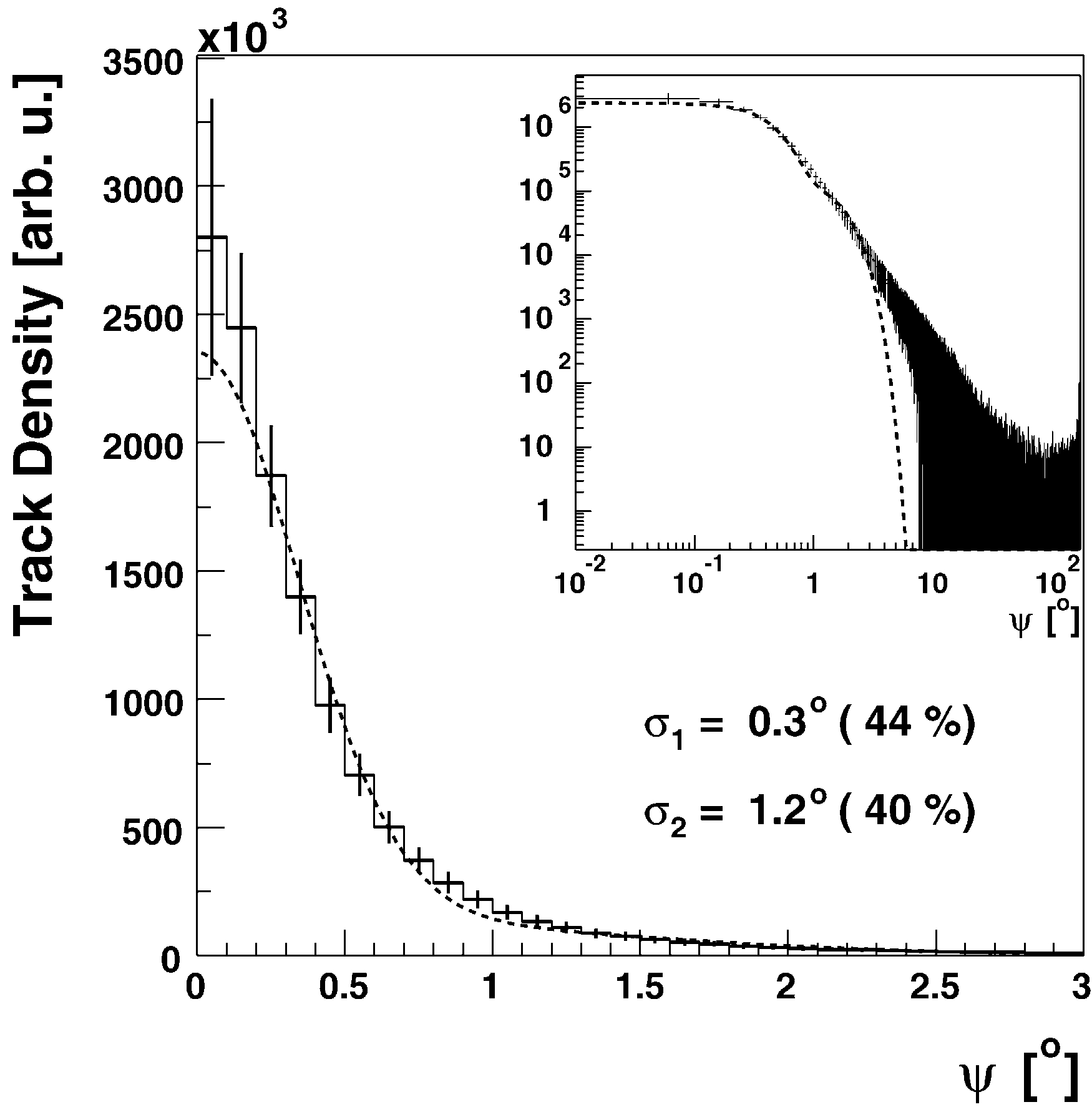
spread function is shown in Fig. 10. This density

distribution is not described well by a single

Gaussian, but can be fitted reasonably well with a

sum of two Gaussians. Such a fit yields standard

deviations of

and

for the two

Gaussians. Integrating the fitted density functions

over the full solid angle shows that the narrower

Gaussian accounts for about 44% of the event

statistics, the broader Gaussian accounts for 40%,

and roughly 16% of the events lie in the tail of the

distribution where the track density is not de-

scribed by a double Gaussian.

5. Sensitivity to astrophysical sources of muon

neutrinos

In most theoretical models, the production of

high-energy cosmic rays is accompanied by the

production of mesons. Prominent candidates for

cosmic-ray sources are putative cosmic accelera-

tors like AGN, microquasars, supernova remnants

and GRBs. Theoretical models for such objects

usually involve shock acceleration of protons. The

Fig. 10.

One-dimensional point-spread function.

The density

distribution, after level 2 selection, of reconstructed tracks

about the true muon direction as a function of the angle

between reconstructed and true track was fitted with the sum of

two Gaussians.

sin

)

–

(

2 1.5 1 0.5 0.5 1.5

–

1.5

0.5

1.5

]

[

)

–

(

1.5

0.5

1.5

]

[

–

1.5

0.5

1.5

Events / Year

01 2

Fig. 9.

Point-spread function in detector coordinates.

The full Monte Carlo event sample of neutrino-induced muons weighted to an

energy spectrum of the initial neutrinos was used after applying level 2 cuts.

J. Ahrens et al. / Astroparticle Physics 20 (2004) 507–532

521

protons interact with ambient matter or radiation

fields producing mesons that subsequently decay

into neutrinos. The spectral distribution of neu-

trinos expected from cosmic accelerators is

, or even harder, depending on the

predominant meson-production mechanism in the

source and on full particulars of the acceleration.

The sum of all cosmic accelerators in the uni-

verse should produce an isotropic flux of high-

energy neutrinos, which would be observable as an

excess above the diffuse flux of atmospheric neu-

trinos. The absolute fluxes from individual sources

may be small, and require careful selection in order

to be resolved. However, in this case, background

can be strongly suppressed since the number of

background events will be reduced with the size of

the spatial search bin or––in case of transient

phenomena––the duration of the observation time

window.

In the following we calculate the sensitivity for

diffuse fluxes of cosmic muon neutrinos as well as

for fluxes from individual point sources, both

steady and transient (GRBs). In contrast to former

analyses, which were based on simple assumptions

on the detector effective area as well as on its en-

ergy resolution [21–23], the method we apply in-

volves exclusively event observables that will be

available from real data taken by IceCube.

5.1. Calculation of the sensitivity

We explore the sensitivity of the IceCube

detector to cosmic neutrino fluxes in two ways.

First we consider the limits that would be placed

on models of neutrino production if no events

were to be seen above those expected from atmo-

spheric neutrinos. Second, we evaluate the level of

source flux required to observe an excess at a given

significance level.

5.1.1. Limit setting potential

Feldman and Cousins have proposed a method

to quantify the ‘‘sensitivity’’ of an experiment

independently of experimental data by calculating

the average upper limit,

, that would be obtained

in absence of a signal [45]. It is calculated from the

mean number of expected background events,

, by averaging over all limits obtained from all

possible experimental outcomes. The average up-

per limit is the maximum number of events that

can be excluded at a given confidence level. That

is, the experiment can be expected to constrain any

hypothetical signal that predicts at least

i¼

signal events.

From the 90% c.l. average upper limit, we define

the ‘‘model rejection factor’’ (

mrf

) for an arbitrary

source spectrum

predicting

signal events, as

the ratio of the average upper limit to the expected

signal [23]. The average flux limit

is found by

scaling the normalization of the flux model

such

that the number of expected events equals the

average upper limit

mrf

5.1.2. Discovery potential

For our purposes, a phenomenon is considered

‘‘discovered’’ when a measurement yields an excess

of 5

over background, meaning that the proba-

bility of the observation being due to an upward

fluctuation of background is less than 2.85

this number being the integral of the one-sided tail

beyond 5

of a normalized Gaussian. From the

background expectation

, we can determine

the minimum number of events

to be observed

to produce the required significance as

obs

iÞ

;

where

obs

iÞ

is the Poisson probability for

observing

obs

background events. The minimum

detectable flux

for any source model can then

be found by scaling the model flux

such that

iþh

i¼

If a real signal source of average strength

present, the probability of the combination of

signal and background producing an observation

sufficient to give the required significance (i.e., an

observation of

events or greater) is

obs

iþh

iÞ

Thus we cannot say that an underlying signal

strength will always produce an observation with

522

J. Ahrens et al. / Astroparticle Physics 20 (2004) 507–532

significance, but we can find the signal strength

such that the probability of

is close to cer-

tainty, e.g., 70%, 90% or 99%.

5.2. Diffuse flux sensitivity

Many models have been developed that predict

a diffuse neutrino flux to be expected from the sum

of all active galaxies in the universe. First we will

consider the potential of IceCube to both place a

limit on, and detect, a generic diffuse flux following

spectrum. After looking in detail at this

case we summarize the capabilities of the detector

to place limits on a few models with spectral

shapes different from

We use the simplest observable related to muon

energy, the multiplicity

of hit channels per

event, for an energy-discrimination cut, in order to

reject the steep spectrum of events induced by

atmospheric neutrinos and retain events from the

harder extraterrestrial diffuse spectrum.

The

correlation between muon energy at closest ap-

proach to the detector center and channel multi-

plicity is shown in the left plot of Fig. 11. The right

plot compares the

distributions for an

signal and atmospheric-neutrino background.

We determine the

cut (rejecting events

below the cut-off) that maximizes the sensitivity

by optimizing the cut with respect to the model

rejection factor (

mrf

) [23]. For each possible cut

value we compute the

mrf

from the number of

remaining signal and background events. The cut

is then applied where the

mrf

is minimized.

This procedure is illustrated in Fig. 12. The left

plot shows the average number of signal and

background events, together with the average

upper limit

, expected from one year

s exposure

to a simulated cosmic-neutrino flux of

GeV as a function of a cut

. The corresponding

mrf

, shown in the right

plot, reaches its minimum of 8.1

for

227, which translates to an overall flux limit

GeV.

This limit applies to the flux of extraterrestrial

muon neutrinos measured at the Earth. In the

presence of neutrino oscillations, the constraint on

the flux escaping cosmic sources must be modified

accordingly. For maximal mixing [46,47] between

muon- and tau-neutrinos during propagation to

the Earth, one would expect the flux of muon

neutrinos at the Earth to be half the flux at the

An improved energy separation is expected from the use of

a more sophisticated energy reconstruction using individual hit

amplitude and/or the full waveform information.

log

(E / GeV)

02 3 4 5 6 7 8

Events / Year

Atm

0 100 200 300 400 500 600 700 800

Fig. 11.

Channel multiplicity.

Left: Correlation between muon energy at closest approach to the detector center and detected channel

multiplicity. The filled squares show the mean number of OMs with at least one recorded hit, averaged over one decade in energy. The

vertical bars indicate the spreads of the corresponding

distributions. Right: Detected channel multiplicity for

signal and

atmospheric background. The signal event rate is normalized to a flux of

GeV.

J. Ahrens et al. / Astroparticle Physics 20 (2004) 507–532

523

source. The limit on the muon-neutrino flux

pro-

duced

in cosmic sources would thus be a factor of

two higher. Here, ‘‘cosmic neutrino flux’’ refers to

the flux of muon neutrinos measured at the Earth.

In the above simulation, in one year 75 signal

events on average are predicted to pass the opti-

mized

cut, compared to eight background

events from atmospheric neutrinos. The back-

ground expectation was calculated using the

rqpm

model for the prompt-charm contribution, ac-

cording to which prompt charm decays account

for 80% of the remaining atmospheric neutrinos.

Using the corresponding prediction based on the

TIG

model would result in an improvement of the

average flux limit by roughly a factor of 2.

The energy spectra of the incident signal and

background neutrinos are shown in Fig. 13. The

final

cut translates into a detection threshold of

about 100 TeV. This threshold results from the

optimization to one particular signal hypothesis,

Cut

Integrated Number of Events

–

0 100 200 300 400 500

mrf

Cut

Minimum : 8.1 * 10

227

0 100 200 300 400 500

Fig. 12.

Optimization of channel multiplicity cut.

Left: Mean number of expected signal (solid) and background (dashed) events in one

year for a model source flux of

GeV, and the corresponding 90% c.l. average upper limit (dotted), as

a function of a cut in channel multiplicity. Right: The model rejection factor calculated from the left plot has a minimum for

227.

Level 2

227

log

/ GeV)

Events / Year

0 1 23 4 5 6 7 8 9 0 1 23 4 5 6 7 8 9

Atm

log

/ GeV)

Events / Year

Fig. 13.

Energy spectra of selected neutrinos

for a diffuse signal flux of

GeV (left) and for atmo-

spheric neutrinos (right), after level 2 cuts (dotted lines) and after application of the optimized

227 cut (solid lines). The cut-off in

the signal spectrum at 10

GeV is due to the limited energy range in the simulation.

524

J. Ahrens et al. / Astroparticle Physics 20 (2004) 507–532

neutrino spectrum extending up to energies

of 10

GeV, where it has an artifical cut-off (the

simulation ends). Extrapolating the signal spec-

trum beyond the cut-off leads to the conclusion

that for an

source a few percent of the final

signal sample would lie at energies above 100 PeV,

provided the flux of neutrinos extends to such high

energies. Without the cut-off in the energy spec-

trum of our simulated event sample, the calculated

sensitivity would be improved at the same scale as

the signal event rate is increased, i.e., the average

upper limit after one year of operation is overes-

timated by a few percent. The effect is stronger for

longer exposure times and for harder spectra, since

the optimal energy-separation cut will be tighter,

shifting the energy threshold towards higher

energies and thereby increasing the fraction of

events with energies above the cut-off.

The sensitivity attained after one year of data

taking is already well below the diffuse bound

calculated by Waxman and Bahcall [48]. (Their

limit holds for optically thin cosmic-ray sources,

under the assumption that these sources produce

the observed flux of high-energy cosmic rays.)

A flux at the level

GeV is needed on average for a 5

detection after a period of one year. This flux is

forty times below the present best established 90%

c.l. upper limit [9].

The improvement with time of the exclusion and

discovery potential of the IceCube detector is

summarized in Table 3. As the exposure time in-

creases, the optimal multiplicity cut becomes tigh-

ter (i.e., higher), resulting in a better separation of

signal and background. After data is taken over

five years instead of one, the sensitivity is improved

by a factor of about 2.5. The 5

detection level

given in Table 3 corresponds to the flux for which

the average event rate from signal plus background

exceeds the 5

threshold. The signal strength at

which the 5

excess is produced at a fixed proba-

bility, is shown in Fig. 14 as a function of time. A

signal of

GeV,

for instance, would be detected with a probability

of 70% after five years of data taking.

Apart from the generic case of an

spectrum,

which is typical for scenarios that involve meson

production in interactions of shock-accelerated

cosmic rays with matter, we have varied the signal

slope towards flatter spectra. Such spectra would be

expected from environments where cosmic rays

predominantly interact on photon fields, e.g., AGN

jets. For each alternative energy spectrum, we

minimized the model rejection factor to find the

cut for which the best sensitivity is attained. From

Table 3

Sensitivity to diffuse neutrino fluxes

Years

cut

(90% c.l.)

1 227 75.4 8.0 6.1 8.1

2.6

3 244 204.8 18.4 8.7 4.2

1.2

5 276 272.5 18.0 8.6 3.2

9.9

Expected limits,

2 d

(90% c.l.), and minimal detectable fluxes,

2 d

, in units of cm

GeV for a generic

source

spectrum. Event numbers correspond to a hypothetical source strength of

GeV.

P(5

) = 70 %

P(5

) = 90 %

P(5

νν

) = 99 %

Years of Data Taking

∗

dN /dE

[

–

GeV

]

90 % C.L. Exclusion

0.5

1.5

2.5

3.5

0 0.5 1 1.5 2 2.5 3 3.5 4 4.5 5

Fig. 14.

Sensitivity to diffuse neutrino fluxes.

Improvement with

time of the diffuse flux with an

spectrum that can be ex-

cluded at 90% c.l. (lower curve) or detected at a 5

level with a

fixed probability

(upper curves).

J. Ahrens et al. / Astroparticle Physics 20 (2004) 507–532

525

the number of background events remaining after

imposing this cut, we determined the event average

upper limit

. As above, the simulated spectrum

was then normalized such that the expected number

of signal events equaled

. The resulting nor-

malization constant is a measure of the detector

sensitivity to signal of this specific spectral shape.

The results obtained for source spectra propor-

tional to

and

are given in Table 4. The

cut was optimized after normalizing the event

samples to a data-taking period of three years. A

signal with a harder energy spectrum allows a

tighter

cut and hence the optimization results in

a lower average upper limit. For an

source

model, the maximum flux which is expected to be

excluded at 90% c.l. after three years of operation

is d

(E/GeV)

This limit is compared to the limit for an

source

spectrum in Fig. 15. The limit that can be placed on

signal hypothesis is d

Table 4

Sensitivity to diffuse neutrino fluxes for alternative source spectra

Source model

cut

Expected 90% c.l. limit

427 3.3 3.1

(E/GeV)

336 4.9 1.5

(E/GeV)

MPR [49] 324 5.2

MPR

S&S [50] 250 8.3

For each energy spectrum, the quoted expected limit is the maximum flux level which is expected to be excluded at 90% c.l. after three

years of data taking. The flux predictions by MPR,

MPR

, and by Stecker and Salamon,

, are still excludable when scaled down by

factors 1.9

and 2.3

(the corresponding model rejection factors after

cut optimization), respectively.

Fig. 15.

Expected sensitivity of the IceCube detector to diffuse neutrino fluxes.

Solid lines indicate the 90% c.l. limit for various dif-

ferential signal energy spectra, calculated for a data-taking period of three years. The lines extend over the energy range containing 90%

of the expected signal. The dashed curve indicates the expected diffuse neutrino flux according to the Stecker and Salamon model for

photo-hadronic interactions in AGN cores [50]. The model rejection factor after three years of data taking for this signal shape is

2.3

. The dotted curve corresponds to the MPR upper bound on neutrino emission from photo-hadronic interactions in AGN jets

[49]. The model rejection factor for this model is 1.9

after three years of data taking. Also shown is the prediction from the GRB

model by Waxman and Bahcall [48] (dash-dotted line).

526

J. Ahrens et al. / Astroparticle Physics 20 (2004) 507–532

(E/GeV)

after three years of oper-

ation.

Mannheim, Protheroe and Rachen (MPR) [49]

have calculated a theoretical upper bound on the

diffuse neutrino flux arising from photo-hadronic

interactions in unresolved AGN jets in the uni-

verse. Their flux bound is shown in Fig. 15 (labeled

MPR

). In order to compare this bound to the

IceCube sensitivity we have computed the model

rejection factor for a hypothetical diffuse signal

with an energy spectrum following this upper

bound. However, since the MPR model extends to

energies well beyond 100 PeV (the artificial cut-off

in the simulation), the simulated signal will not

include events predicted at the highest energies.

The model rejection factor for the MPR model

(

100 PeV) is 1.9

after three years of

data taking, meaning that after this period Ice-

Cube will be sensitive to fluxes of similar spectral

shape, but fifty times lower than the MPR bound.

Finally, we have selected one particular model

by Stecker and Salamon [50] for neutrinos from

proton interactions on the UV thermal photon

field in AGN cores. The corresponding diffuse flux

prediction is labeled

in Fig. 15. The model

rejection factor corresponding to three years of

data taking is in this case 2.3

5.3. Sensitivity to point sources

An excess of events from a particular direction

in the sky suggests the existence of a point source.

The ability of the detector to reconstruct muon

tracks to within 1

of their true direction allows a

search window to be used with a size that greatly

reduces the background, while retaining a large

fraction of the signal. This allows a loosening of

the energy-separation cut.

We restrict this analysis to the case of a point-

source search for candidate sources in the northern

sky. That is, we do not simulate a cluster or grid

search, but instead consider the case where an

angular search bin is fixed by the direction of

the candidate source under scrutiny. In reality the

sensitivity will depend on the declination of the

source location. For simplicity of presentation we

calculate averaged event rates for all declinations

throughout the northern sky.

We use an angular search cone with a 1

opening half-angle centered about the direction of

a hypothetical point source (i.e., we allow an

angular deviation of 1

in any direction). After

application of the standard cut selection (level 2),

we again optimize the

cut with respect to the

model rejection potential for a point source fol-

lowing an

spectrum. A cut at a channel mul-

tiplicity of

30, combined with the angle cut

of one degree, leads to the best average flux upper

limit of

GeV

after one year of data taking. A flux three times

greater will on average produce a 5

signal.

Table 5 and Fig. 16 summarize the improvement

of the limit with increased exposure time. After

three years of operation IceCube can be expected to

place flux limits on potential sources at a level of

GeV, while

the discovery probability for a flux three times

stronger is higher than 70%. After five years of

operation a source emitting a flux of

GeV would be ob-

served at 5

significance with a probability of 70%.

As in the case of a diffuse signal, we have varied

the energy spectrum for the signal hypothesis in

order to see how it affects the sensitivity to point

sources. The results listed in Table 6 correspond to

three years of data taking.

Table 5

Sensitivity to neutrino point sources

Years

cut

(90% c.l.)

1 30 62.8 1.4 3.6 5.5

1.7

3 40 142.3 1.3 3.5 2.4

7.2

5 42 213.7 1.4 3.6 1.7

4.9

Expected limits,

2 d

90%c

, and minimal detectable fluxes,

2 d

, in units of cm

GeV for a generic

source spectrum

and different exposure times. Signal event rates correspond to a hypothetical source strength of

GeV.

Background event rates include

rqpm

charm neutrinos.

J. Ahrens et al. / Astroparticle Physics 20 (2004) 507–532

527

Fig. 17 shows the energy spectra of both

the remaining signal events and the remaining

events from the atmospheric-neutrino back-

ground after applying standard level 2 cuts and

after cutting at

30. This selection results

in an effective energy threshold of about 1 TeV.

Since most of the signal in this case is in the

TeV–PeV range, the energy cut-off at 10

GeV

in the simulation has a negligible impact on the

result. The shown results are valid for the

rqpm

prediction for prompt neutrinos. Using

the

TIG

model improves the sensitivity by about

2%.

5.4. Gamma ray burst sensitivity

Although the progenitors of GRBs are un-

known, observations indicate the existence of a

fireball. The coexistence of nucleons and photons

P(5

) = 70

P(5

) = 90

P(5

) = 99

Years of Data Taking

/dE

[

–

GeV

]

C.L. Exclusion

0.5

1.5

2.5

3.5

0 0.5 1 1.5 2 2.5 3 3.5 4 4.5 5

∗

Fig. 16.

Sensitivity to pointlike neutrino emission.

Improvement

with time of the point-source flux with an

source spectrum

that can be excluded at 90% c.l. (lower curve) or detected at a 5

level with a fixed probability

(upper curves).

Table 6

Sensitivity to point-source fluxes for various source energy spectra

Source model

cut

Expected 90% c.l. limit

58 2.7 2.4

(E/GeV)

49 2.9 4.5

(E/GeV)

40 3.5 2.4

(E/GeV)

24 6.1 3.8

(E/GeV)

For each energy spectrum, the quoted expected limit is the maximum flux level which is expected to be excluded at 90% c.l. after three

years of data taking.

Level 2

log

/ GeV)

Events / (Year*Bin)

Atm

log

/ GeV)

Events / (Year*Bin)

02 3

45 6 7 8 9

02 3

45 6 7 8 9

Fig. 17.

Energy spectra of selected neutrinos

for a point-source signal with an assumed flux of

GeV (left)

and for atmospheric neutrinos including

rqpm

charm (right). The selection corresponds to level 2 cuts (dotted lines) and additional

application of the optimized cut

30 (solid lines). The spatial search bin was defined by an angular cone with a 1

opening half-

angle.

528

J. Ahrens et al. / Astroparticle Physics 20 (2004) 507–532

in the fireball may result in the production of

neutrinos.

Waxman and Bahcall [48] calculated the ex-

pected flux of neutrinos from the sum of all GRBs

by assuming that they are the source of the ob-

served flux of cosmic rays. The Waxman–Bahcall

model results in a broken power-law neutrino

spectrum given by

;

where the break energy

lies at

GeV. Above

GeV the spectrum steepens again by one

power in energy. With a full-sky GRB rate of

1000 per year, as assumed by Waxman and Bah-

call, the normalization constant in Eq. (5) would

amount to

GeV.

This

neutrino flux is shown in Fig. 15 (labeled

GRB

). It

appears to be below the diffuse-flux sensitivity level

of IceCube. However, the search for neutrinos

accompanying GRBs is essentially background-

free, due to the requirement that the neutrino events

are coincident in both direction

and

time with sa-

tellite observations of the gamma rays.

The search for neutrinos from GRB sources

involves summing over the observation time and

spatial search windows for many separate bursts.

For this analysis we have used a hypothetical

observation duration of 10 s and a spatial search

cone of 10

(opening half-angle) centered about the

direction of each GRB. We have only considered

events in the northern sky, where the search is not

limited by downward cosmic-ray-muon back-

ground. From 500 bursts in 2

sr (out of the 1000

assumed over the full sky in one year) we would

expect 13 neutrino-induced upward muons per year

after applying standard level 2 quality cuts. The

background of atmospheric neutrinos is strongly

reduced by the spatial and temporal coincidence

requirements. With almost full retention of the

signal (

i¼

3 after imposing the coincidence

requirements), the atmospheric neutrino back-

ground expectation is reduced to roughly 0.1 event.

This low background expectation allows the exclu-

sion of signals of mean intensity

5 events

per year at 90% classical confidence, which trans-

lates into a model rejection factor of

mrf

meaning that the experiment will be sensitive to a

neutrino flux with roughly one fifth of the intensity

originally calculated by Waxman and Bahcall

(Table 7). This, in turn, means that a sample of 100

observed bursts would suffice to exclude the Wax-

man and Bahcall model. A 5

detection would re-

quire the observation of

5 neutrino events,

which corresponds to the mean number of events

expected from 203 bursts. In this case the proba-

bility to actually observe a 5

excess is about 58%.

With 500 bursts this probability climbs to 99%.

The time period after which we can expect a

detection depends on the efficiency of gamma-ray

observations, since the search strategy requires the

GRBs to trigger satellite-borne detectors. Assum-

ing that future gamma-ray observations will pro-

vide a few hundred triggered bursts per year, we

can conclude that IceCube has excellent prospects

to reveal the neutrino signal possibly emerging

from gamma-ray bursters within a very short time.

The analysis of data taken over one year would

presumably suffice to yield a 5

signal, provided

the model by Waxman and Bahcall predicts neu-

trino fluxes at the right scale. Moreover, the sen-

sitivity given above is obtained when employing

the most conservative search strategy, namely

searching only one hemisphere for the signal of

upward neutrinos. However, the drastic back-

ground reduction that follows from restricting the

search to a short time window about each ob-

served GRB

s detection time will result in a sizable

acceptance also for signal from above the horizon.

5.5. Systematic uncertainties and possible improve-

ments

The systematic uncertainty in the given flux

limits is presently dominated by three components.

The largest is an uncertainty in the angular

dependence of the OM sensitivity, including the

effect of the refrozen ice around the OM. A local

A more recent calculation yielded a normalization constant

which is about three times larger [51]. The event rates given here

do not include this factor, since we have used the normalization

originally calculated by Waxman and Bahcall in [48].

J. Ahrens et al. / Astroparticle Physics 20 (2004) 507–532

529

increase in light scattering from air bubbles trapped

in the vicinity of the OM translates into a modu-

lation of its angle-dependent acceptance. This

component is followed in size by uncertainties in

the absolute OM sensitivity and uncertainties re-

lated to modeling and implementation of the

optical properties of the bulk ice in the simulation.

For the comparatively small AMANDA-B10 array

the inclusion of all components of uncertainty

weakens the point source flux limit by 25% com-

pared to when the nominal simulation values are

used [52]. The variation of some of these parame-

ters in simulations of the larger AMANDA-II

array and for IceCube indicates that for larger

arrays the systematic uncertainties of the basic

input parameters become less important, except for

muon energies close to the detection threshold. For

instance, increasing the absolute OM sensitivity in

IceCube by a factor of two results in a 25% (10%)

larger effective area at 1 (10) TeV. Taking into ac-

count that uncertainties in limits depend weaker-

than-linearly on uncertainties in effective area [52],

we estimate the overall uncertainties in the limits

for

signal derived above to be at most 20%.

However, a number of improvements of detec-

tor properties will reduce the systematic uncer-

tainties and enhance the performance of IceCube

compared to AMANDA. Using glass spheres and

PMTglass with higher UV transparency or, alter-

natively, covering the glass spheres with wave-

length-shifting film, will increase the OM sensitivity

in the UV range and improve light collection. This

will increase the overall sensitivity and angular

resolution, particularly at

low energies

. Informa-

tion extracted from the full PMTwaveforms

will

improve both angular resolution and energy

reconstruction at

high energies

. Finally, the inclu-

sion of information provided by the IceTop surface

array will enhance the rejection power with respect

to downward-moving atmospheric muons. This

tool, unique to IceCube, is expected to be particu-

larly helpful for rejecting events with coincident

muons from independent air showers and would

allow the loosening of other rejection criteria,

thereby enhancing the signal efficiency.

6. Summary

We have described the expected performance of

the IceCube detector in searching for muons from

extraterrestrial neutrinos in the TeV–PeV energy

range.

A Monte Carlo simulation of a realistic model

detector was used to assess the sensitivity of the

experiment. We simulated both neutrino-induced

muons and muons produced from cosmic-ray

interactions in the atmosphere with sufficient sta-

tistics to establish event-selection criteria and to

infer expected event rates for each event class. The

trigger rate due to downward muons produced in

the atmosphere was found to be 1.7 kHz, including

a 50 Hz rate due to uncorrelated air showers that

produce time-coincident muons within the detec-

tor. Muons induced by atmospheric neutrinos are

expected to cause about 0.8 million triggers per

year. A benchmark flux of

GeV for the diffuse signal of astro-

physical neutrinos results in 3300 triggers per year.

Roughly one third of these events pass a set of

standard quality cuts which at the same time re-

duces the background rate from misreconstructed

downward-going muon tracks to the level of well-

reconstructed upward-moving muons from atmo-

spheric neutrinos.

Table 7

Sensitivity to neutrino fluxes in coincidence with GRBs

GRBs Time window Angular cone

Flux limit

500 10 s 10

12.3 0.1 2.5 0

Average numbers of signal and background events expected for a sample of 500 observed GRBs, given a neutrino spectrum

(as defined in Eq. (5)) and an intensity as calculated by Waxman and Bahcall in [48]. The event numbers are summed

over all temporal and spatial search windows centered about each GRB. A neutrino flux following this energy spectrum is expected to

be excludable by IceCube at an intensity 0.2 times the intensity originally calculated by Waxman and Bahcall.

Waveform information will be available also in AMANDA

data from 2003 onward.

530

J. Ahrens et al. / Astroparticle Physics 20 (2004) 507–532

In order to quantify the detector acceptance,

we have computed the effective detector area for

muons. After applying the standard quality crite-

ria, the effective area exceeds one square kilometer

for upward-moving muons with energies above 10

TeV. At this level of data reduction, 50% of all

muons with these energies will be reconstructed

with an accuracy of 0.8

or better. For energies

above 100 TeV, the angular acceptance with

respect to well-identified extraterrestrial neutrinos

extends above the horizon and the effective area

reaches 0.6 km

for near-vertical downward

muons in the PeV range. This means that at high

energies IceCube can observe a large part of the

Galaxy, including the Galactic center.

In order to quantify the sensitivity to fluxes of

astrophysical neutrinos, we have determined the

flux normalization for a generic

differential

energy spectrum that corresponds to a detection

with 5

significance, or, in absence of signal, a 90%

c.l. limit. We found a diffuse source strength of

GeV for the 5

detection level and 4

GeV for

the exclusion potential of the detector, given an

observation time of three years. This is two orders

of magnitude below present experimental limits.

For pointlike neutrino emission we found that,

after three years, a flux of

GeV would result in a 5

excess over

background, while a flux of

GeV could be excluded at 90% c.l.

Both numbers are averaged over all declinations

throughout the northern sky. Integrated over all

neutrino energies above 1 TeV, these fluxes trans-

late to

1TeV

Þ¼

Þ?

We have also calculated the potential of Ice-

Cube to detect neutrinos in coincidence with GRB,

following the model of Waxman and Bahcall. We

found that a 5

signal is expected from the

observation of about 200 bursts, while an obser-

vation of 100 bursts would suffice to rule out the

Waxman and Bahcall model.

Acknowledgements

This research was supported by the following

agencies: National Science Foundation––Office of

Polar Programs, National Science Foundation––

Physics Division, University of Wisconsin Alumni

Research Foundation, USA; Swedish Research

Council, Swedish Polar Research Secretariat,

Knut and Alice Wallenberg Foundation, Sweden;

German Ministry for Education and Research,

Deutsche Forschungsgemeinschaft (DFG), Ger-

many; Fund for Scientific Research (FNRS-

FWO), Flanders Institute to encourage scientific

and technological research in industry (IWT),

Belgian Federal Office for Scientific, Technical and

Cultural affairs (OSTC), Belgium; Inamori Science

Foundation, Japan; FPVI, Venezuela; The Neth-

erlands Organization for Scientific Research

(NWO).

References

[1] T.K. Gaisser, F. Halzen, T. Stanev, Phys. Rep. 258 (1995)

173.

[2] J.G. Learned, K. Mannheim, Ann. Rev. Nucl. Part. Sci. 50

(2000) 679.

[3] C. Spiering, Prog. Particle Nucl. Phys. 48 (2002) 43.

[4] P.K.F. Grieder et al., Nucl. Phys. Proc. Suppl. 43 (1995)

145.

[5] V.A. Balkanov et al., Nucl. Phys. Proc. Suppl. 75A (1999)

409.

[6] E. Andres et al., Astropart. Phys. 13 (2000) 1.

[7] J. Ahrens et al., Phys. Rev. D 66 (2002) 012005.

[8] I.A. Belolaptikov et al., Phys. Atom. Nucl. 63 (2000) 951.

[9] J. Ahrens et al., Phys. Rev. Lett. 90 (2003) 251101.

[10] T. Montaruli et al., in: Proceedings of the 26th ICRC, vol.

2, 1999, p. 213.

[11] E. Aslanides et al., A Deep Sea Telescope for High Energy

Neutrinos, Proposal, 1999. Available from <astro-ph/

9907432>.

[12] S. Bottai, in: Proceedings of the 26th ICRC, vol. 2, 1999,

p. 456.

[13] G. Riccobene, in: Proceedings of the Workshop on

Methodical Aspects of Underwater/Ice Neutrino Tele-

scopes, DESY-PROC-2002-01, 2002, p. 61.

[14] J. Ahrens et al., The IceCube NSF Proposal, 2000.

[15] A. Biron et al., Participation of DESY-Zeuthen in the

IceCube Project, Proposal to the DESY PRC, 2001.

[16] J. Ahrens et al., IceCube Conceptual Design Document,

2001.

[17] A. Goldschmidt, in: Proceedings of the 27th ICRC, vol. 3,

2001, p. 1237.

[18] M. Leuthold, in: Proceedings of the Workshop on Simu-

lation and Analysis Methods for Large Neutrino Tele-

scopes, DESY-PROC-1999-01, 1999, p. 484.

[19] H. Wissing, Diploma thesis, Humboldt Universit

€

at zu

Berlin, 2001.

J. Ahrens et al. / Astroparticle Physics 20 (2004) 507–532

531

[20] X. Bai et al., in: Proceedings of the 27th ICRC, vol. 3,

2001, p. 981.

[21] I.F.M. Albuquerque, J. Lamoureux, G. Smoot. Available

from <hep-ph/0109177>.

[22] J. Alvarez-Muniz, F. Halzen, Phys. Rev. D 63 (2001) 037302.

[23] G.C. Hill, K. Rawlins, Astropart. Phys. 19 (2003) 393.

[24] A.Bouchta et al., 2002. Available from <http://www.ifh.de/

nuastro/software/siegmund/siegmund.html>.

[25] S.N. Boziev et al., INR-Preprint 0630, 1989.

[26] D. Heck, J. Knapp, Extensive Air Shower Simulation with

CORSIKA: A User

s Guide, Forschungszentrum Kar-

lsruhe, Institut f

€

ur Kernphysik, 2000.

[27] C.G.S. Costa, Astropart. Phys. 16 (2001) 193.

[28] T. Gaisser, M. Honda, Ann. Rev. Nucl. Part. Sci. 52 (2002)

153.

[29] G.C. Hill, Ph.D. thesis, University of Adelaide, 1996.

[30] A.D. Martin, W.J. Stirling, R.G. Roberts, Phys. Lett. B

354 (1995) 155.

[31] A.M. Dziewonski, D.L. Anderson, Phys. Earth Planet.

Interiors 25 (1981) 297.

[32] P. Lipari, T. Stanev, Phys. Rev. D 44 (1991) 3543.

[33] P. Lipari, Astropart. Phys. 1 (1993) 195.

[34] E.V. Bugaev et al., Phys. Rev. D 58 (1998) 054001.

[35] M. Thunman, G. Ingelman, P. Gondolo, Astropart. Phys.

5 (1996) 309.

[36] G. Gelmini, P. Gondolo, G. Varieschi, Phys. Rev. D 61

(2000) 036005; Phys. Rev. D 61 (2000) 056011.

[37] J. Ahrens et al., Phys. Rev. D 67 (2003) 012003.

[38] W. Lohmann, R. Kopp, R. Voss, CERN Yellow Report

85-03, 1985.

[39] A. Karle, in: Proceedings of the Workshop on Simulation

and Analysis Methods for Large Neutrino Telescopes,

DESY-PROC-1999-01, 1999, p. 174.

[40] S. Hundermark, in: Proceedings of the Workshop on

Simulation and Analysis Methods for Large Neutrino

Telescopes, DESY-PROC-1999-01, 1999, p. 276.

[41] S. Hundertmark, Ph.D. thesis, Humboldt-Universit

€

at zu

Berlin, 1999.

[42] V.J. Stenger, DUMAND internal Report HDC-1-90, 1990.

[43] J. Ahrens et al., NIM, submitted.

[44] C. Wiebusch, in: Proceedings of the Workshop on Simu-

lation and Analysis Methods for Large Neutrino Tele-

scopes, DESY-PROC-1999-01, 1999, p. 302.

[45] G.J. Feldman, R.D. Cousins, Phys. Rev. D 57 (1998) 3873.

[46] Y. Fukuda et al., Phys. Rev. Lett. 81 (1998) 1562.

[47] Q.R. Ahmad et al., Phys. Rev. Lett. 87 (2001) 071301.

[48] E. Waxman, J. Bahcall, Phys. Rev. D 59 (1999) 023002.

[49] K. Mannheim, R.J. Protheroe, J.P. Rachen, Phys. Rev. D

63 (2001) 023003.

[50] F.W. Stecker, M.H. Salamon, Space Sci. Rev. 75 (1996)

341.

[51] E. Waxman, Nucl. Phys. Proc. Suppl. 118 (2003) 353.

Available from <astro-ph/0211358>.

[52] J. Ahrens et al., Astrophys. J. 583 (2003) 1040.

532

J. Ahrens et al. / Astroparticle Physics 20 (2004) 507–532