Measurement of the cosmic ray composition at the knee
with the SPASE-2/AMANDA-B10 detectors
AMANDA and SPASE Collaborations
J. Ahrens
a
, M. Ackermann
b
, E. Andres
c
, X. Bai
d,1
, S.W. Barwick
e,
*
,
R.C.Bay
f
,T.Becka
a
,K.-H.Becker
g
,E.Bernardini
b
,D.Bertrand
h
,F.Binon
h
,
A. Biron
b
, D.J. Boersma
b
,S.B
€
oser
b
, O. Botner
i
, A. Bouchta
i
, O. Bouhali
h
,
T. Burgess
j
, S. Carius
k
, T. Castermans
l
, D. Chirkin
f
, J. Conrad
i
, J. Cooley
c
,
D.F. Cowen
m
, A. Davour
i
, C. De Clercq
p
, T. DeYoung
c,2
, P. Desiati
c
,
J.-P. Dewulf
h
, E. Dickinson
n,1
, P. Ekstr
€
om
j
, R. Engel
d,3
, P. Evenson
d,1
,
T. Feser
a
, T.K. Gaisser
d,1
, R. Ganugapati
c
, M. Gaug
b
, H. Geenen
g
,
L. Gerhardt
e
, A. Goldschmidt
o
, A. Hallgren
i
, F. Halzen
c
, K. Hanson
c
,
R. Hardtke
c
, T. Hauschildt
b
, M. Hellwig
a
, P. Herquet
l
, G.C. Hill
c
,
J.A. Hinton
n,1
, D. Hubert
p
, B. Hughey
c
, P.O. Hulth
j
, K. Hultqvist
j
,
S.Hundertmark
j
,J.Jacobsen
o
,A.Karle
c
,J.Kim
e
,L.K
€
opke
a
,M.Kowalski
b
,
K. Kuehn
e
, J.I. Lamoureux
o
, H. Leich
b
, M. Leuthold
b
, P. Lindahl
k
,
I. Liubarsky
q
, J. Lloyd-Evans
n,1
, J. Madsen
r
, K. Mandli
c
, P. Marciniewski
i
,
H.S. Matis
o
, C.P. McParland
o
, T. Messarius
g
, T.C. Miller
d,4
, Y. Minaeva
j
,
P. Mio
?
cinovi
?
c
f,5
, P.C. Mock
e,6
, R. Morse
c
, R. Nahnhauer
g
, T. Neunh
€
offer
a
,
P. Niessen
p
, D.R. Nygren
o
,H.
€
Ogelman
c
, Ph. Olbrechts
p
,
C.P
?
erezdelosHeros
j
,A.C.Pohl
j
,R.Porrata
e,7
,P.B.Price
f
,G.T.Przybylski
o
,
K. Rawlins
c
, E. Resconi
b
, W. Rhode
g
, M. Ribordy
b
, S. Richter
c
,
K.Rochester
n,1
,J.Rodr
?
ıguezMartino
j
,D.Ross
e
,H.-G.Sander
a
,T.Schmidt
b
,
K. Schinarakis
g
, S. Schlenstedt
b
, D. Schneider
c
, R. Schwarz
c
, A. Silvestri
e
,
M. Solarz
f
, G.M. Spiczak
r,1
, C. Spiering
b
, M. Stamatikos
c
, T. Stanev
d,1
,
*
Corresponding author. Fax: +1-949-824-2174.
E-mail address:
sbarwick@uci.edu(S.W. Barwick).
1
SPASE Collaboration.
2
Department of Physics, University of Maryland, College Park, MD 20742.
3
Present address: Forschungszentrum Karlsruhe, Institut fur Kernphysik, Postfach 3640, 76021 Karlsruhe, Germany.
4
Present address: Applied Physics Laboratory, Johns Hopkins University, Laurel, MD 20723, USA.
5
Department of Physics and Astronomy, University of Hawaii, Honolulu, HI 96822, USA.
6
Present address: SEA Inc. 7545 Metropolitan Dr. San Diego, CA 92108, USA.
7
Present address: L-174, Lawrence Livermore National Laboratory, 7000 East Ave., Livermore, CA 94550, USA.
0927-6505/$ - see front matter
?
2004 Elsevier B.V. All rights reserved.
doi:10.1016/j.astropartphys.2004.04.007
Astroparticle Physics 21 (2004) 565–581
www.elsevier.com/locate/astropart
D. Steele
c
, P. Steffen
b
, R.G. Stokstad
o
, K.-H. Sulanke
b
, I. Taboada
s
,
S. Tilav
d,1
, C. Walck
j
, W. Wagner
g
, Y.-R. Wang
c
, A.A. Watson
n,1
,
C.H. Wiebusch
g
, C. Wiedemann
j
, R. Wischnewski
b
, H. Wissing
b
,
K. Woschnagg
f
,W.Wu
e
, G. Yodh
e
, S. Young
e
a
Institute of Physics, University of Mainz, Staudinger Weg 7, D-55099 Mainz, Germany
b
DESY-Zeuthen, D-15735 Zeuthen, Germany
c
Department of Physics, University of Wisconsin, Madison, WI 53706, USA
d
Bartol Research Institute, University of Delaware, Newark, DE 19716, USA
e
Department of Physics and Astronomy, University of California, Irvine, CA 92697, USA
f
Department of Physics, University of California, Berkeley, CA 94720, USA
g
Fachbereich 8 Physik, BUGH Wuppertal, D-42097 Wuppertal, Germany
h
Universit
?
e
Libre de Bruxelles, Science Faculty CP230, Boulevard du Triomphe, B-1050 Brussels, Belgium
i
Division of High Energy Physics, Uppsala University, S-75121Uppsala, Sweden
j
Department of Physics, Stockholm University, SCFAB, SE-10691 Stockholm, Sweden
k
Department of Technology, Kalmar University, S-39182 Kalmar, Sweden
l
Universit
?
e
de Mons-Hainaut, 19 Avenue Maistriau 7000, Mons, Belgium
m
Department of Physics, Pennsylvania State University, University Park, PA 16802, USA
n
School of Physics and Astronomy, University of Leeds, Leeds LS2 9JT, UK
o
Lawrence Berkeley National Laboratory, Berkeley, CA 94720, USA
p
Vrije Universiteit Brussel, Dienst ELEM, B-1050 Brussel, Belgium
q
Imperial College, London SW7 2AZ, UK
r
Department of Physics, University of Wisconsin, River Falls, WI 54022, USA
s
Departamento de Fı
´
sica, Universidad Simon Bolı
´
var, Apdo. Postal 89000, Caracas, Venezuela
Received 6 February 2004; accepted 5 April 2004
Available online 26 May 2004
Abstract
The mass composition of high-energy cosmic rays at energies above 10
15
eV can provide crucial information for the
understanding of their origin. Air showers were measured simultaneously with the SPASE-2 air shower array and the
AMANDA-B10 Cherenkov telescope at the South Pole. This combination has the advantage to sample almost all high-
energy shower muons and is thus a new approach to the determination of the cosmic ray composition. The change in
the cosmic ray mass composition was measured versus existing data from direct measurements at low energies. Our data
show an increase of the mean log atomic mass
h
ln
A
i
by about 0.8 between 500 TeV and 5 PeV. This trend of an
increasing mass through the ‘‘knee’’ region is robust against a variety of systematic effects.
?
2004 Elsevier B.V. All rights reserved.
Keywords:
Cosmic Rays; Neutrino astronomy; Mass composition
1. Introduction
Cosmic rays observed at Earth follow a steep
power-law spectrum over many orders of magni-
tude in energy. At an energy of approximately
3 PeV, however, the spectral index steepens; this
feature is called the ‘‘knee’’. To understand the
reason for the knee, one must understand the
source, acceleration mechanism, and propagation
of cosmic rays. For instance, first-order Fermi
acceleration, thought to explain cosmic rays below
the knee, has a natural cutoff energy which de-
pends on the rigidity of the nucleus being accel-
erated. Observing the mass composition of cosmic
rays at the knee therefore provides an important
clue to the origin of cosmic rays.
The study of high-energy cosmic rays has led to
the construction of large ground-based air shower
566
J. Ahrens et al. / Astroparticle Physics 21 (2004) 565–581
arrays to explore the energy range above 100 TeV
where the cosmic ray flux is too low for direct
measurements. These arrays, unlike satellite- or
balloon-borne instruments, must reconstruct the
properties of primary cosmic rays indirectly, from
the behavior of the extensive air shower particles
produced in the atmosphere. The different particle
components of an air shower (electrons, photons,
muons, and hadrons) can be measured using dif-
ferent detection techniques. Since the behavior of
any one particle component generally depends on
both primary energy and primary mass, multi-
component measurements are proving to be a
powerful detection tool.
One such multicomponent experiment is
SPASE/AMANDA, a scintillator array and deep-
ice Cherenkov telescope working in coincidence at
the South Pole. SPASE measures the electron
component of the air showers at the surface, while
AMANDA measures muon bundles at depths of
1500–2000 m. By combining electron and muon
information, the primary cosmic ray energy and
mass can be estimated for each coincidence event.
2. The SPASE and AMANDA detectors
The South Pole Air Shower Experiment
(SPASE-2, or SPASE in this paper) is a scintillator
array consisting of 120 modules grouped into 30
stations on a 30 m triangular grid. The SPASE site
on the surface lies about 400 m from the center of
the AMANDA hole locations, at an atmospheric
depth of
?
685g cm
?
2
[1].
The Antarctic Muon And Neutrino Detector
Array (AMANDA) uses the natural ice at the
South Pole as the target and detection volume for
a large-scale Cherenkov telescope [2]. Currently,
an array of 677 optical modules (OM’s) containing
photomultipliers is frozen in the ice. This work
uses data from 1998, in which the detector com-
prised 302 OM’s on 10 strings between depths of
1500 and 2000 m. The OM’s measure the Cher-
enkov light emitted by charged particles traveling
faster than the speed of light in ice. AMANDA’s
primary mission is the detection of high-energy
neutrinos by collecting Cherenkov light emitted by
their interaction product, a lepton such as a muon.
A neutrino-induced muon is only identifiable by its
upgoing direction. Misreconstructed downgoing
cosmic ray muons (produced in the atmosphere
above the South Pole) constitute the dominant
background for neutrino-induced muons, and so
great care is taken to remove them from neutrino
analyses. In this work, however, cosmic ray muons
are the
signal
, rather than the background. Some
difficulties of the neutrino analysis can be avoided
here, while a cosmic ray analysis presents new and
different challenges of its own.
3. Shower reconstruction in SPASE
SPASE data analysis reconstructs the shower
direction from the arrival times of charged parti-
cles in the array’s scintillators. The shower core
location and shower size are reconstructed by fit-
ting the lateral distribution of particle density to
the Nishimura–Kamata–Greisen (NKG) function
[3] and then evaluating this lateral distribution at a
fixed distance from the shower core. In particular,
SPASE data analysis computes for each event the
shower parameter
S
(30), the measured particle
density at 30 m from the shower core, in units of
equivalent minimum ionizing vertical muons per
m
2
. The shower core can be reconstructed within a
few meters, and the shower direction to within 1.5
?
at low energies, improving to less than 0.4
?
at
higher energies [4].
S
(30) can be used as an energy
estimator, but it is not entirely composition-inde-
pendent. The shower size depends also on the
height of interaction in the atmosphere, which in
turn depends on the primary mass. A detailed
description of how
S
(30) is measured can be found
in references [1,5].
4. Reconstruction in AMANDA
Just as SPASE is used to reconstruct the posi-
tion, direction, and electron size of an air shower
event, a similar procedure is developed for the
analysis of the muon bundle in AMANDA. First,
the combined detectors are used to get the bundle’s
position and direction more accurately than can be
achieved using either detector alone. Then, the
J. Ahrens et al. / Astroparticle Physics 21 (2004) 565–581
567
expected lateral distribution function (LDF) of
photons from a muon bundle is computed. Two
corrections must be applied to the LDF in order to
be able to apply it to all OM’s and all depths. The
first accounts for the ranging-out of muons be-
tween the top of the detector and the bottom. The
second accounts for the changing scattering length
in the ice, due to variation of concentration of
impurities such as dust in ice. For each event, the
LDF is fitted to OM amplitudes and evaluated at a
fixed distance of 50 m from the center of the
bundle to compute a parameter called
K
ð
50
Þ
. This
parameter is analogous to
S
(30) but measures
muon energy loss rather than electron density. The
technique is described in more detail below.
4.1. Track reconstruction
The standard AMANDA track reconstruction,
described in [6], is performed by the reconstruction
program recoos. To reconstruct muon direction in
normal operation, recoos varies the position
ð
x
;
y
;
z
Þ
of a point on the track and its direction
ð
h
;
/
Þ
, until the track hypothesis (a single muon
line source) is most likely to have given rise to the
observed light pattern. SPASE coincidences,
however, provide additional information: the
shower core location at the surface (within 3–4 m)
and shower direction (within 1.5
?
). A better track
can be found by fixing the track position at the
reconstructed shower core in SPASE, using SPA-
SE’s reconstructed track as a first guess, and
allowing
recoos
to vary
only
the direction angles
ð
h
;
/
Þ
as free parameters. The long lever arm be-
tween the two detectors (about 1750 m center-
to-center) gives this technique great accuracy, less
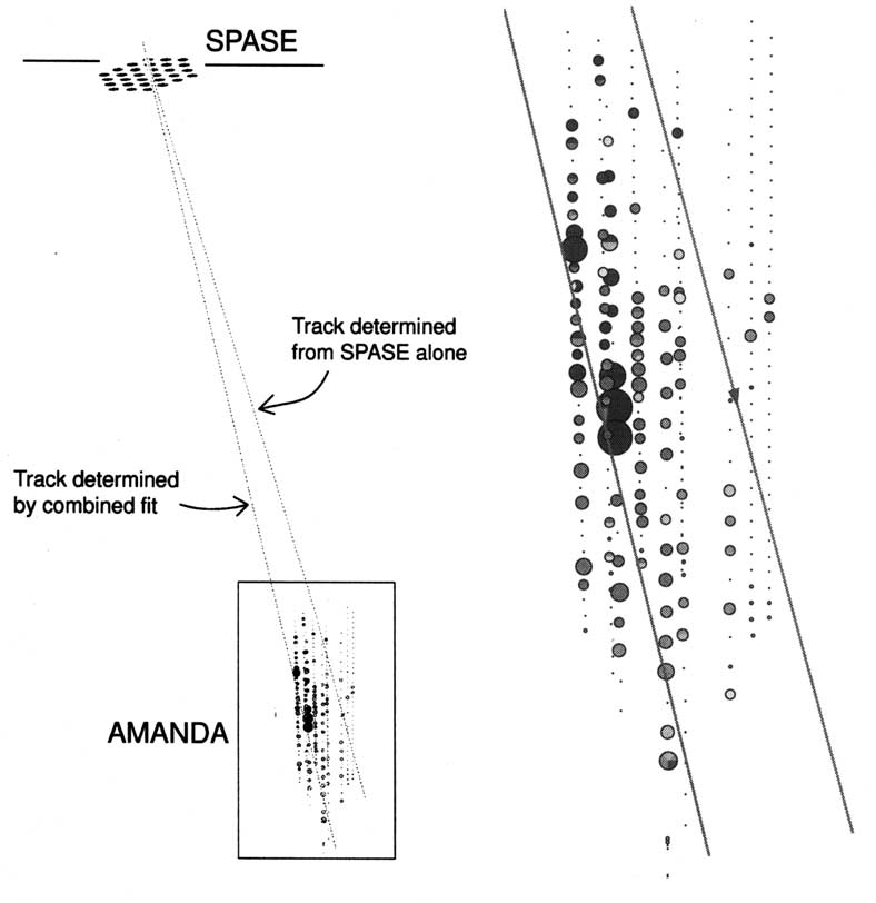
than a half degree. Fig. 1 shows the relative posi-
tions of SPASE and AMANDA, and how the
SPASE reconstruction alone can be improved by
using both detectors with this combined technique.
Fig. 1. SPASE/AMANDA coincidence event from 1997 data.
568
J. Ahrens et al. / Astroparticle Physics 21 (2004) 565–581
4.2. Muons in AMANDA
High-energy muons (meaning in this context,
muons of energy above 300 GeV which can reach
the detector at depth) are created by the decay of
high-energy charged pions and kaons originating
high in the atmosphere in the early stages of
shower development. The Gran Sasso laboratories
(housing the underground LVD and MACRO
experiments) have explored the potential of coin-
cidences between surface electrons from EAS-TOP
and TeV muons [7–10]. Due to their small size,
MACRO and similar experiments sample only a
few individual muons from the air shower.
AMANDA is shallower (resulting in a lower muon
energy threshold) and also much larger. It can also
detect light up to 150 m from the muon bundle.
AMANDA can measure the energy loss of the
muon bundle at depth, but it is too sparse an array
to resolve individual muons. This makes AMAN-
DA a fundamentally different kind of cosmic ray
detector, requiring new techniques. Therefore in
this paper we must devote some time to the physics
of muon bundles emitting light in ice, and the
introduction of a new technique for reconstructing
the total muon energy loss using photomultiplier
pulse amplitudes recorded by AMANDA.
The differential energy spectrum of the muons
in a shower at the surface follows a power law with
spectral index
)
2.757 [11]. As the muons penetrate
the ice, their energy loss can be described by [12]
?
d
E
l
d
x
¼
a
eff
þ
b
eff
E
l
ð
1
Þ
with values of
a
eff
and
b
eff
for ice also taken from
[12]. From the surface spectrum and this differen-
tial equation, one can calculate the distribution of
the number of muons surviving to slant depth
X
N
l
depth
ð
X
Þ¼
N
l
surface
ð
>
E
Þ¼
KE
?
1
:
757
¼
K
a
eff
b
eff
??
ð
e
b
eff
X
?
?
1
Þ
?
?
1
:
757
ð
2
Þ
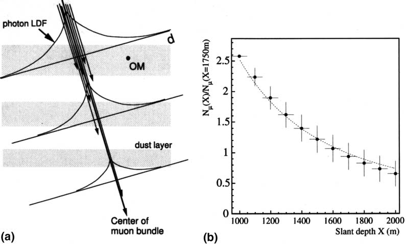
This equation also describes how the muon
intensity within a single event changes as the
bundle propagates through the detector from 1500
m at the top to 2000 m at the bottom, illustrated in
Fig. 2(a). Simulations of muons propagating
through these depths of ice are compared in Fig.
2(b) to this simple functional form, which will be
used later for computing the range-out correction
to the photon LDF.
Only muons with a surface energy of more than
?
300 GeV survive to AMANDA depth. The
transverse momentum of these muons is small
Fig. 2. Propagation of muons through the ice: (a) schematic representation of how the ranging out of muons affects the photon LDF;
(b) ratio of muons reaching slant depth
X
, as a function of
X
, averaged over many simulated events. The fraction is defined to be
relative to the arbitrary reference slant depth of 1750 m, which is the distance from the center of SPASE to the center of AMANDA.
Dashed line: Muon fraction calculated using Eq. (2) in the text.
J. Ahrens et al. / Astroparticle Physics 21 (2004) 565–581
569
compared to their longitudinal momentum, so the
muons are tightly contained in a bundle. Simula-
tions show that on average 90% of all muons
reaching the detector level are contained within a
radius of
?
20 m in 1 PeV proton-induced showers.
In iron-induced showers of the same energy this
radius increases to
?
30 m.
4.3. Light from muons in ice
At the wavelengths relevant to AMANDA,
between 300 and 600 nm, impurities (dust) are the
most important contributor to both absorption
and scattering of light in deep Antarctic ice. A
YAG laser at a wavelength of 532 nm was first
used to map the effective scattering length,
k
e
, and
the absorption length,
k
a
, as functions of depth
[13], revealing vertical fluctuations due to dusty
layers of ice. More recently,
in-situ
light emitters at
a variety of other wavelengths (470 nm with blue
LEDs, 370 nm with UV LEDs, and 337 nm with a
Nitrogen laser) [14] have confirmed the predicted
wavelength dependence of both scattering [15] and
absorption [16].
For a
line
source of light, the photon intensity
seen by an OM is the integrated contribution from
many infinitesimal length elements. At distances
d
large compared to
k
e
the photon intensity is de-
scribed by a modified Bessel function of the second
kind [16]:
I
ð
d
Þ/
1
k
e
K
0
ð
d
=
k
Þ
;
ð
3
Þ
where
d
is the perpendicular distance from the OM
to the primary track, and
k
is an effective propa-
gation length due to the combined effects of
absorption and scattering, given by
k
¼
ffiffiffiffiffiffiffiffiffiffiffiffiffiffi
k
e
k
a
=
3
p
/
k
e
ð
4
Þ
For large enough values of its argument
z
, the
Bessel function
K
0
, can be approximated as
ffiffiffiffiffiffiffiffiffiffiffiffiffiffi
2
=
ð
p
z
Þ
p
e
?
z
. The photon LDF for a particular ice
layer can then be described by:
I
ð
d
Þ/
1
k
ffiffiffiffiffiffiffiffi
d
=
k
p
e
?
d
=
k
¼
1
ffiffiffiffiffiffiffiffi
d
=
k
p
e
?
d
=
k
ð
5
Þ
At large distances, photons have been travelling
through ice layers of different quality, which to-
gether can be described by a bulk ice propagation
length
k
¼
k
0
. At near distances, the propagation
length of the OM’s local ice layer
k
¼
k
ð
z
Þ¼
c
ice
ð
z
Þ
k
0
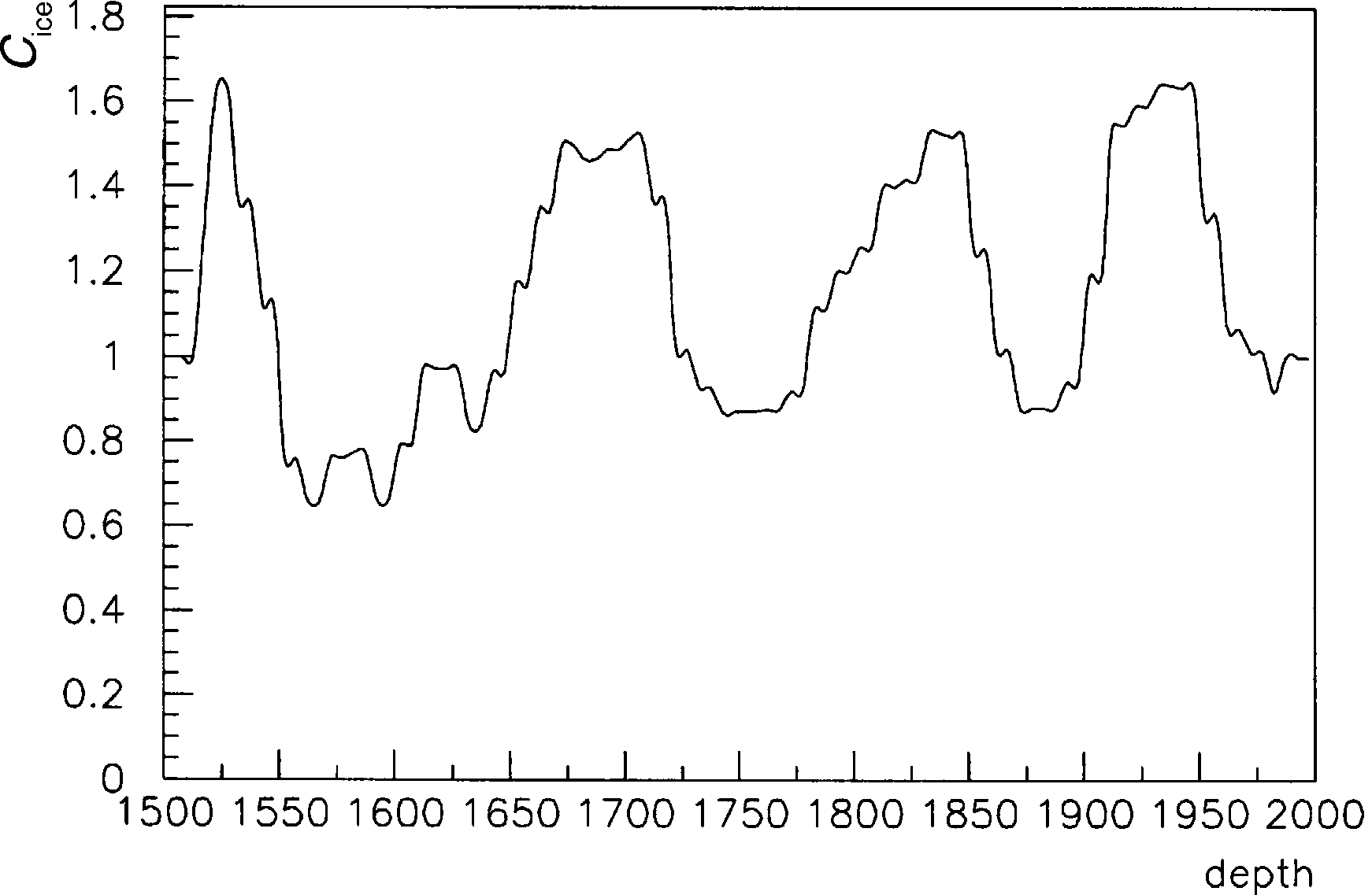
is more appropriate. The depth-depen-
dent correction factor
c
ice
ð
z
Þ
, shown in Fig. 3, is
taken from in-ice measurements of the variation of
scattering length around the average value [13].
For an approximate treatment of the effect of dust
layers at
all
distances, the photon LDF can be
described by a split function which employs
k
ð
z
Þ
below a transition distance
D
and
k
0
above it
I
ð
z
;
d
Þ/
1
ffiffiffiffiffiffiffiffiffiffiffiffiffiffiffiffiffiffiffi
k
0
c
ice
ð
z
Þ
d
p
e
?
d
=
ð
k
0
c
ice
ð
z
ÞÞ
;
d
<
D
1
ffiffiffiffiffiffiffi
k
0
d
p
e
?
d
=
k
0
;
d
>
D
8
>
>
>
<
>
>
>
:
ð
6
Þ
This functional form fits well to data when a
value of 80 m, which is comparable to the spacing
between depths with peak concentration of dust, is
used for the transition distance
D
.
4.4. Complete LDF fit
The complete photon LDF for all depths and
distances incorporates both the range-out correc-
tion and the ice correction. An expected OM
amplitude
A
, follows the same functional form
and is proportional to the LDF intensity
A
¼
NN
l
depth
ð
X
Þ
I
ð
z
;
d
Þð
7
Þ
where the overall normalization,
N
, absorbs other
normalization factors and also converts the result
Fig. 3. The ice correction
C
ice
as a function of depth, from in-
ice scattering data.
570
J. Ahrens et al. / Astroparticle Physics 21 (2004) 565–581
into units of OM amplitude (photoelectrons).
N
is
also proportional to the total amount of light
emitted by the muon bundle.
With the track position and direction held fixed,
recoos maximizes the likelihood
L
of the ampli-
tudes measured by AMANDA modules to derive
from the expected functional form:
L
¼
Y
all OM
0
s
L
OM
¼
Y
all OM
0
s
P
ð
A
measured
j
A
Þ
;
ð
8
Þ
where
P
is a Poisson probability. The overall
normalization
N
and the bulk propagation length
k
0
are left as free parameters.
N
is proportional to
the total energy loss of muons in the ice.
k
0
is
known from in-ice measurements to be about 26 m
[13]. However, errors in track reconstruction can
cause a change in the best-fit slope of the LDF. If
instead we fit
k
0
as a free parameter and then
evaluate the resulting reconstructed LDF at a fixed
distance, we can achieve a very stable measure-
ment of the overall muon energy loss. The recon-
structed
k
0
can also be used as a cut parameter to
ensure that the LDF for the fitted event has been
reconstructed sensibly.
The fit LDF is evaluated at a constant distance,
in this case 50 m; this distance offers the most
stable measurement under simultaneous variations
in fitted
N
and
k
0
due to errors in track recon-
struction. The parameter
K
50 is defined as
the value of the fit LDF function, evaluated in
the absence of correction factors (meaning
N
l
depth
ð
X
Þ¼
1and
c
ice
ð
z
Þ¼
1), and at a distance of
50 m from the primary track
K
50
¼
N
ffiffiffiffiffiffiffiffiffiffiffiffiffiffiffiffiffiffiffi
ð
50 m
Þ
k
0
p
e
?ð
50 m
Þ
=
k
0
:
ð
9
Þ
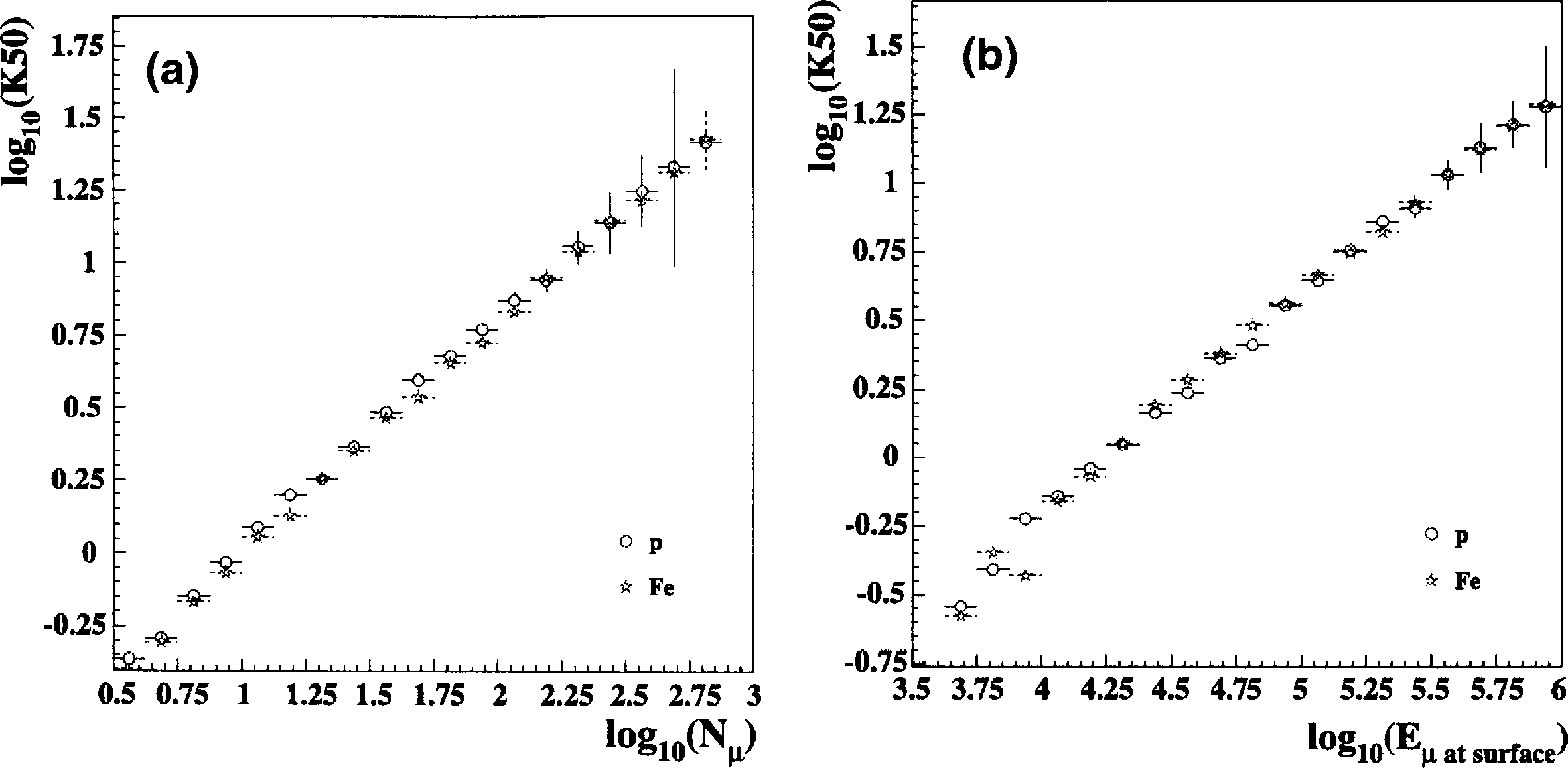
K
50 is analogous to similar parameters used by
other experiments, and is a measurement of muon
energy loss. This parameter is also well-correlated
with the number of muons in the bundle, shown in
Fig. 4(a), and with the total muon energy at the
surface, shown in Fig. 4(b) (see Section 5.2 for a
description of the simulation procedure). These
correlations are nearly composition-independent.
K
50 is not, however, a direct measurement of the
number of muons that reach the detector, since it
also accounts for the emission and propagation of
the Cherenkov light through the ice that surrounds
the AMANDA optical modules.
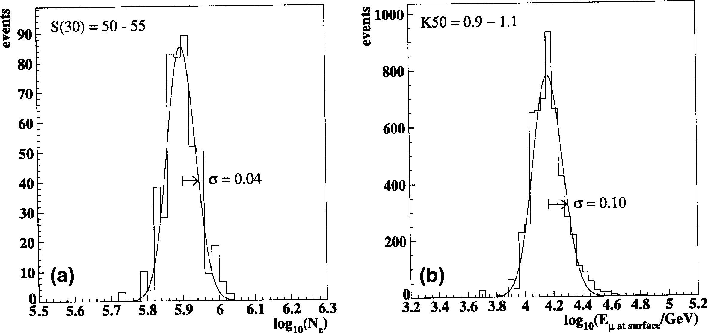
Fig. 5 shows the resolutions of the two
parameters we will use together to measure cosmic
ray energy and mass:
S
ð
30
Þ
and
K
50. A measure-
ment of
S
ð
30
Þ
in SPASE relates to the total num-
ber of electrons in the shower, with a resolution
shown in Fig. 5 (a): 0.04 in log
10
ð
N
e
Þ
for
S
ð
30
Þ
between 50 and 55 m
?
2
. A measurement of
K
50
in AMANDA relates to the total muon energy,
with a resolution shown in Fig. 5(b) 0.10 in
log
10
(
E
l
at surface
Þ
for
K
50 between 0.9 and 1.1 pho-
toelectron/OM. It may be noted that an event of
this brightness generates a total of about 300
photoelectrons summed over all OM’s.
Fig. 4. The reconstructed
K
50 resolution, for proton and iron simulations (the irregularity at low energies is a small-statistics fluc-
tuation): (a)
K
50 vs. the true number of muons at 1750 m slant depth and (b)
K
50 vs. the true total muon energy at the surface.
J. Ahrens et al. / Astroparticle Physics 21 (2004) 565–581
571
5. Data and Monte Carlo samples
5.1. Data
SPASE/AMANDA coincidence data from 1998
were used for the results in this work (though data
from 1997 were used first to explore the tech-
niques). AMANDA operated in slave mode to
SPASE, reading out all OM’s upon receiving an
SPASE trigger externally. Events were matched
together offline by comparing GPS times (each
detector has its own independent clock) and
requiring a match within 1 ms. A more detailed
description of how SPASE and AMANDA oper-
ate in coincidence can be found in [17]. Coinci-
dence events between SPASE and AMANDA
have zenith angles of between 8
?
and 18
?
,with
additional quality cuts confining this range even
further.
5.2. Monte Carlo simulations
The simulation used in this work employs a
modified version of the air shower code MOCCA
[18] using the QGSJET98 interaction model [19].
We simulated 350 000 proton- and iron-induced
showers according to an
E
?
1
spectrum from ener-
gies of 100 TeV to about 100 PeV, and from angles
of 0
?
to 30
?
. The events are re-weighted to a cosmic
ray energy spectrum, with a spectral index of
)
2.7
below a knee at 3 PeV and
)
3.0 above it. The
surface component is processed through the
SPASE detector simulation. Whenever SPASE is
triggered by the simulated air shower, the SPASE
scintillator data together with the muon informa-
tion are recorded. The high-energy muons are then
propagated through the ice with the muon prop-
agator PROPMU [20]. The Cherenkov photons
generated by the muon are finally propagated
through the ice and events are simulated with a
detailed AMANDA detector simulation. The sys-
tematic uncertainties associated with these simu-
lations will be discussed further on, together with
the results.
5.3. Quality cuts
A small set of quality cuts ensures an event
sample where both SPASE and AMANDA have
reliably reconstructed the track direction and the
parameters
S
ð
30
Þ
and
K
50.
•
The shower is large enough to reconstruct size
.
Small showers are not well reconstructed, so an
iterative determination of
S
ð
30
Þ
is not performed
when the first determination gave
S
ð
30
Þ
<
4
m
?
2
. All events with
S
ð
30
Þ
less than m
?
2
are dis-
carded in this analysis at an early stage.
•
The track passes within the AMANDA array
.
SPASE tracks which pass
outside
AMANDA
tend to get pulled
in
by the combined track fit
described in Section 4.1. Thus, we require the
Fig. 5. Resolutions of
S
ð
30
Þ
reconstructed by SPASE, and
K
50 reconstructed by AMANDA (simulated p,He,O,and Fe nuclei all
included): (a) shower size resolution: The distribution of true total number of electrons is shown for events with
S
ð
30
Þ
in the range 50–
55 m
?
2
and (b) muon energy resolution: the distribution of true total muon energy at the surface is given for a
K
50 in the range 0.9–1.1
photoelectron/OM.
572
J. Ahrens et al. / Astroparticle Physics 21 (2004) 565–581
SPASE track of an event to intersect a cylinder
of ice representing AMANDA’s geometrical
volume.
•
The shower core lies within the SPASE array
. The
shower core reconstruction and therefore the
entire event reconstruction is not reliable if
the core is located outside the array. The cut
removes about 10% of the data.
•
For small
S
ð
30
Þ
showers, the track must pass clo-
ser to the center of AMANDA
. Angular resolu-
tion begins to suffer for small
S
ð
30
Þ
when fewer
AMANDA modules are hit. However, tracks
which pass close to the center of AMANDA
can still be reconstructed well. Between
S
ð
30
Þ¼
5 and 20 m
?
2
, the cut on track direction
is tightened linearly from 1.0 to 0.7 times the
geometrical size of AMANDA, in order to pre-
serve good angular resolution without losing
too many events.
•
The LDF fit slope is within a reasonable range
.
As discussed earlier, the reconstructed effective
propagation length
k
0
should resemble what
has been independently measured for antarctic
ice, but can take on a range of values and still
provide a robust
K
50. This slope is required
to be between zero and 100. This cut does not
have a large impact on the event statistics; it
merely removes unphysical outliers.
In 1998 SPASE recorded 28.9 million showers.
AMANDA’s ontime during that year was 70% of
SPASE’s. Out of the coincidentally recorded
events 16% were pointing at AMANDA and pas-
sed the
S
ð
30
Þ
>
5
m
?
2
cut. 70,000 of those events
were succesfully reconstructed, and 5655 events
survive the additional quality cuts to the final
analysis level. From the Monte Carlo sample, 5515
events survive to this level.
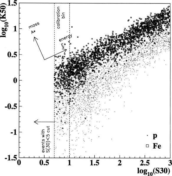
6. Measuring cosmic ray energy and composition
When the two observables
K
50 and
S
ð
30
Þ
are
plotted against each other, as in Fig. 6, showers of
different primary energy and primary mass can be
separated in the two-dimensional parameter space.
The higher the primary energy of the event, the
more electrons in SPASE and the more muons in
AMANDA. But for a
given
primary energy, iron-
induced showers are more muon-rich than proton-
induced showers and
K
50 is enhanced relative to
S
ð
30
Þ
. This can be explained in a simplified way by
the superposition principle; a shower from a nu-
cleus of mass
A
can be approximated as
A
super-
imposed proton-like showers, each with 1
=
A
of the
total primary energy. The larger the
A
, the smaller
the energy fraction carried by each nucleon, and
the lower the energies of secondary pions, which
are more likely to decay into muons before inter-
acting. Thus, heavy primaries produce more muons
for the same primary energy than light primaries.
We can create a set of transformed axes, named
E
?
and
A
?
, also shown in Fig. 6. These axes are
rotated from
K
50 and
S
(30) by an angle (deter-
mined by simulations) of 24
?
. Every event can now
be identified with coordinates in
E
?
?
A
?
space,
and these coordinates are used as energy and mass
estimators for that event.
Two more steps are necessary to get to a
determination of
h
ln
A
i
itself. First, the absolute
scale of
K
50 (the more vulnerable of the two ob-
servables to systematic uncertainties) must be cal-
ibrated. This is done by calibrating the mass
Fig. 6.
S
ð
30
Þ
vs. JFC50 for simulated proton and iron events.
The ‘‘calibration bin’’ of
S
ð
30
Þ
between 5 and 10 m
?
2
, as well as
the directions of the
A
?
and
E
?
axes are indicated on the plot.
J. Ahrens et al. / Astroparticle Physics 21 (2004) 565–581
573
composition at low energies where direct mea-
surements are available. Second, the data and
Monte Carlo simulations are then compared along
the
E
?
and
A
?
axes to get the best fit mass com-
position in a series of energy bins.
The analysis presented here uses a 2-component
Monte Carlo model (proton and iron primaries).
The data are expected to lie somewhere in be-
tween, and the mean log mass
h
ln
A
i
from a mix-
ture of protons and iron is used to characterize the
mass composition. A 4-component model (p, He,
O, and Fe) was also explored, and is used here as a
consistency check.
6.1. Calibrating with direct measurements at low
energy
To measure the absolute scale of
K
50 from
simulations alone suffers systematic uncertainties
from a variety of sources, for instance, the absolute
number of muons predicted by the hadronic inter-
action model or the muon propagation simulation.
These uncertainties affect the absolute calibration
of the
K
50 parameter, but not the shape or prop-
erties of its distribution. Cosmic ray composition is
known at low energies from direct measurements
up to several hundred TeV; if we calibrate the
measurement at low energies to agree with the
known composition, we can then investigate whe-
ther the composition
changes
as energy increases.
The technique is calibrated at low energies using
events with
S
ð
30
Þ¼
5–10 m
?
2
, the vertical ‘‘slice’’
shown in Fig. 6, which corresponds to 200–350
TeV protons and about twice this energy for iron.
Monte Carlo events, which are generated over a
wide energy range using the same spectral index
for each component, are weighted by a relative
proportion which represents a mixed composition,
or
h
ln
A
i
. This mean log mass at low energy can be
taken from direct measurements such as JACEE
[21] and RUNJOB [22]. Figure 19 of Ref. [22]
shows
h
ln
A
i
of 2.1
?
0.2 measured by JACEE be-
tween 10
5
and 10
6
GeV and
h
ln
A
i¼
1
:
7
?
0
:
3
measured by RUNJOB. We have taken a calibra-
tion value
h
ln
A
i¼
2.
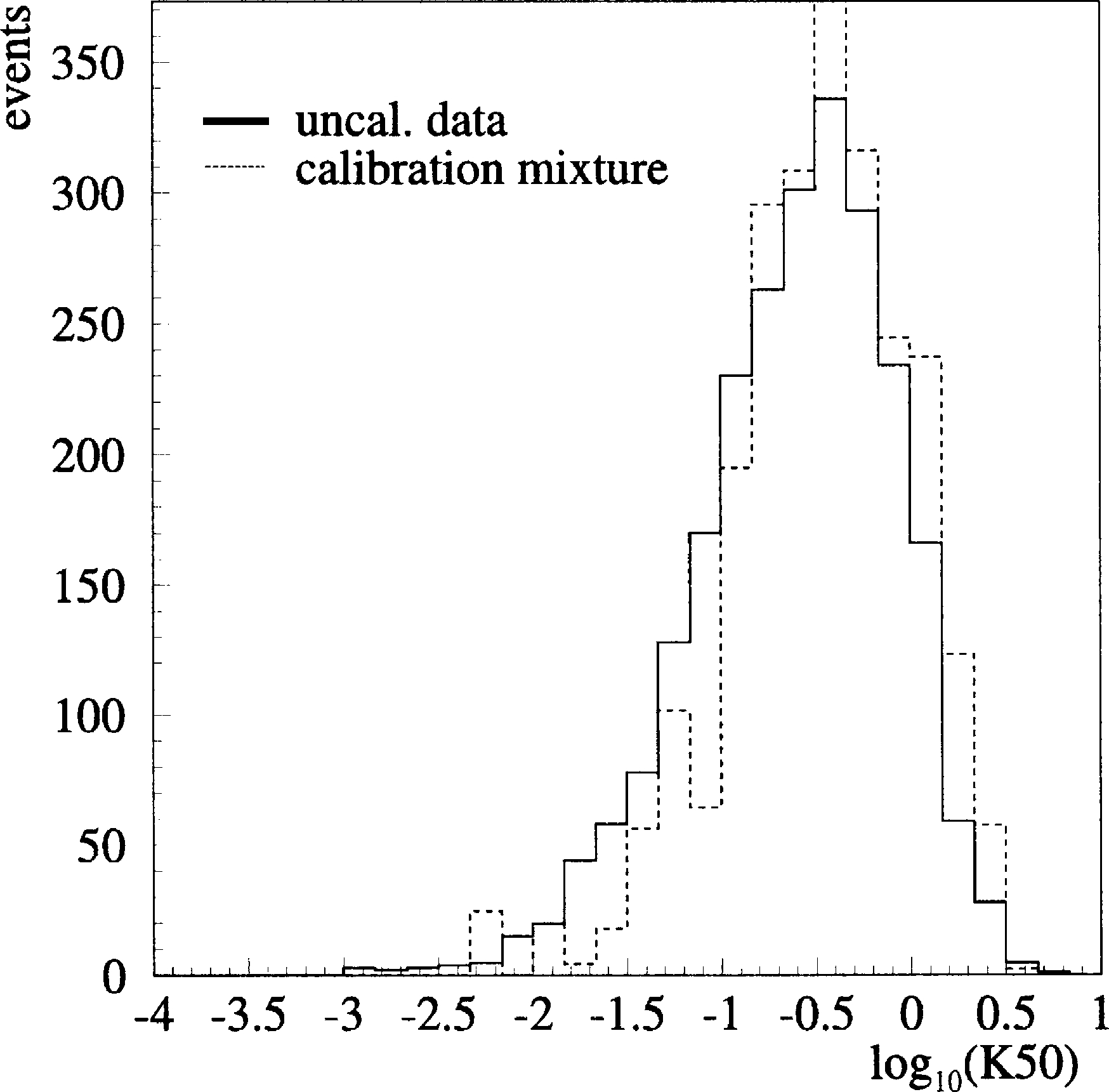
The distributions of log
10
ð
K
50
Þ
for data and the
calibration mixture of simulated proton and iron
within this slice, shown in Fig. 7, agree well in
shape, but not in mean. Hypothesizing that data
and Monte Carlo differ by a constant offset
?
in
log
10
ð
K
50
Þ
, we can find the value of
?
which makes
the two histograms agree best using a Kolmogo-
rov–Smirnov test. This renormalization factor is
applied to the log
10
ð
K
50
Þ
of the data for the
remainder of this paper. For the baseline model,
?
is found to be 0.14. Alternative values of
?
were
also analyzed in order to investigate systematic
errors; these will be discussed later.
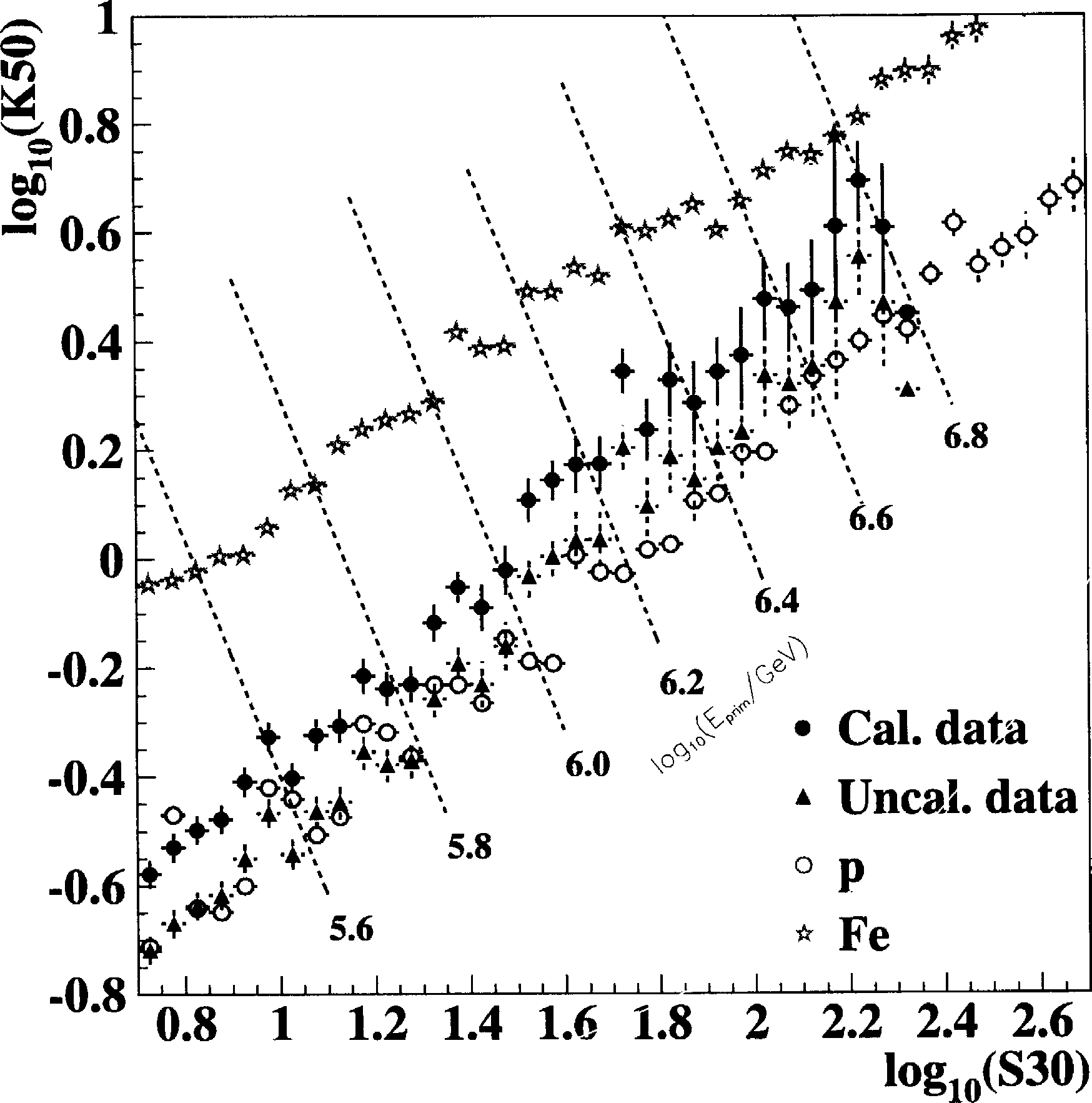
Fig. 8 shows both calibrated and uncalibrated
data in the
K
50
?
S
ð
30
Þ
parameter space, together
with the simulated proton and iron events. Un-
calibrated, the data appear unphysically light
given our knowledge of mass composition at low
energies. Calibrated, the data reveal the trend in
mass composition. The seven slanted straight lines
drawn represent the constant energies of log
10
(
E
prim
=
GeV
Þ¼
5
:
6, 5.8, 6.0, 6.2, 6.4, 6.6, and 6.8.
They form six
bins
of constant energy. A formal
procedure for measuring energy and mass is de-
scribed below.
6.2. Energy resolution
The
E
?
axis is roughly linear in the log of
the true primary energy. Using simulations, we
Fig. 7. The distribution of log
10
(
K
50) for uncalibrated data and
the calibration mixture.
574
J. Ahrens et al. / Astroparticle Physics 21 (2004) 565–581
compare this energy estimator with the true pri-
mary energy log
10
(
E
prim
). The relationship is com-
position-independent, and can be fit by
log
10
ð
E
prim
=
GeV
Þ¼
4
:
9
þ
0
:
72
?
E
?
ð
10
Þ
The resolution of this line fit is given in Table 1
for five different energy ranges with equal mixtures
of proton- and iron-induced showers:
r
¼
0
:
12 in
log
10
ð
E
prim
Þ
at energies near 100 TeV, and
improving 0.057 at the highest simulated energies
of 30 PeV. The combined detector’s response is
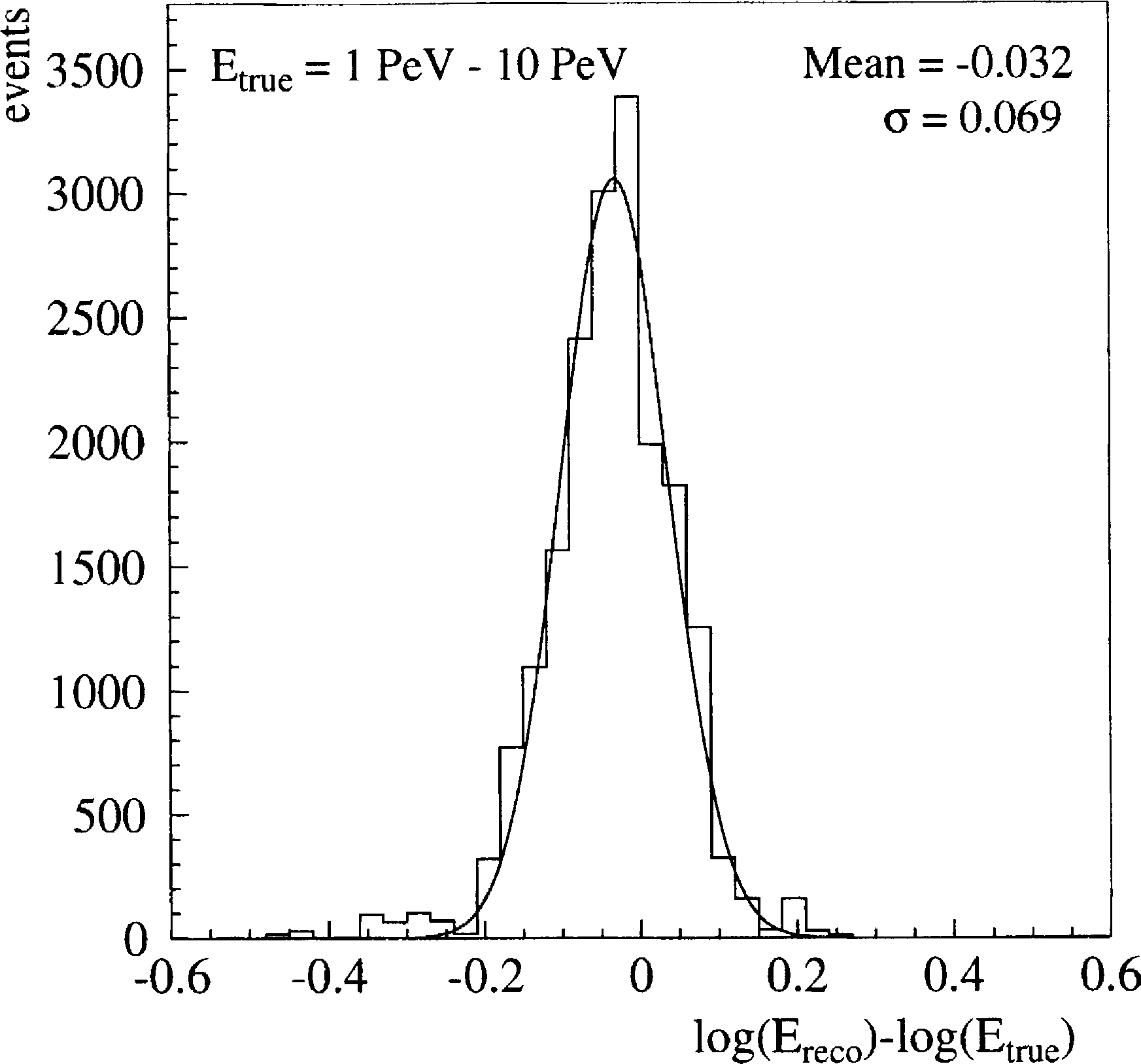
linear up to about 10 PeV. Fig. 9 shows the energy
resolution of proton- and iron-induced air showers
in the energy range from 1 to 10 PeV. The average
energy resolution is
r
¼
0
:
07 in log
10
(
E
prim
).
6.3. Mass resolution
Just as
E
?
can be used to estimate primary en-
ergy,
A
?
can be used to estimate primary mass for
each shower. In particular, to measure cosmic ray
composition from the data, we compare the
A
?
distributions of the data and the Monte Carlo. The
proton and iron Monte Carlo events can be mixed
with an iron fraction
f
Fe
to reproduce a given
h
ln
A
i
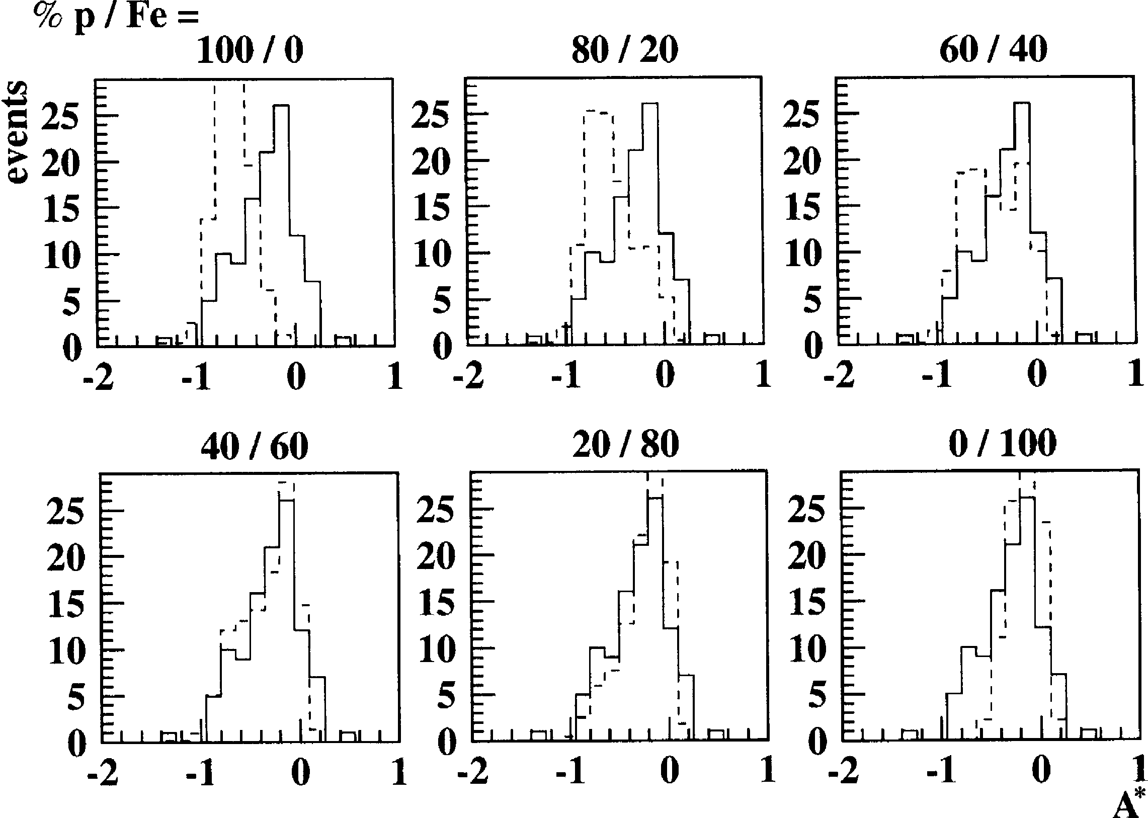
. The mixture which best describes the data is
found by scanning through hypothesis mixtures,
such as those shown in Fig. 10. The likelihood
L
of each hypothesis
f
Fe
is the product over histo-
gram bins of the Poisson probability of observing
the number of data events given the number of
simulated events in that bin. The most likely
f
Fe
is
found at the peak of the resulting likelihood curve,
where
L
ð
f
Fe
Þ¼
L
max
. The error on the measure-
ment can be derived from the width of the likeli-
hood curve; if
L
is Gaussian in
f
Fe
, then 1
r
is the
value of
f
Fe
at which [23]
Fig. 8. Uncalibrated and calibrated data, in the
K
50
?
S
ð
30
Þ
parameter space, compared to simulated proton and iron
events. Constant-energy contours are also shown.
Table 1
Energy resolution of an equal mixture of p- and Fe-induced
showers as a function of energy based on full detector simula-
tion of both detectors
log
10
ð
E
=
GeV
Þ
log
10
ð
E
reco
=
E
true
Þ
lr
5.0–5.5 0.010 0.119
5.5–6.0
)
0.041 0.113
6.0–6.5
)
0.035 0.072
6.5–7.0
)
0.014 0.059
7.0–7.5
)
0.026 0.057
Fig. 9. Distributions of the differences between reconstructed
and true energy of an equal mixture of p- and Fe-showers for
the energy range from 1 to 10 PeV. The width of the distribu-
tion measures the energy resolution. The results are based on
full shower and detector Monte Carlo simulations.
J. Ahrens et al. / Astroparticle Physics 21 (2004) 565–581
575
ln
L
ð
f
Fe
Þ¼
ln
L
max
exp
"
?
ð
1
r
Þ
2
2
r
2
!#
¼
ln
L
max
?
1
=
2
ð
11
Þ
The simulated histograms are normalized to the
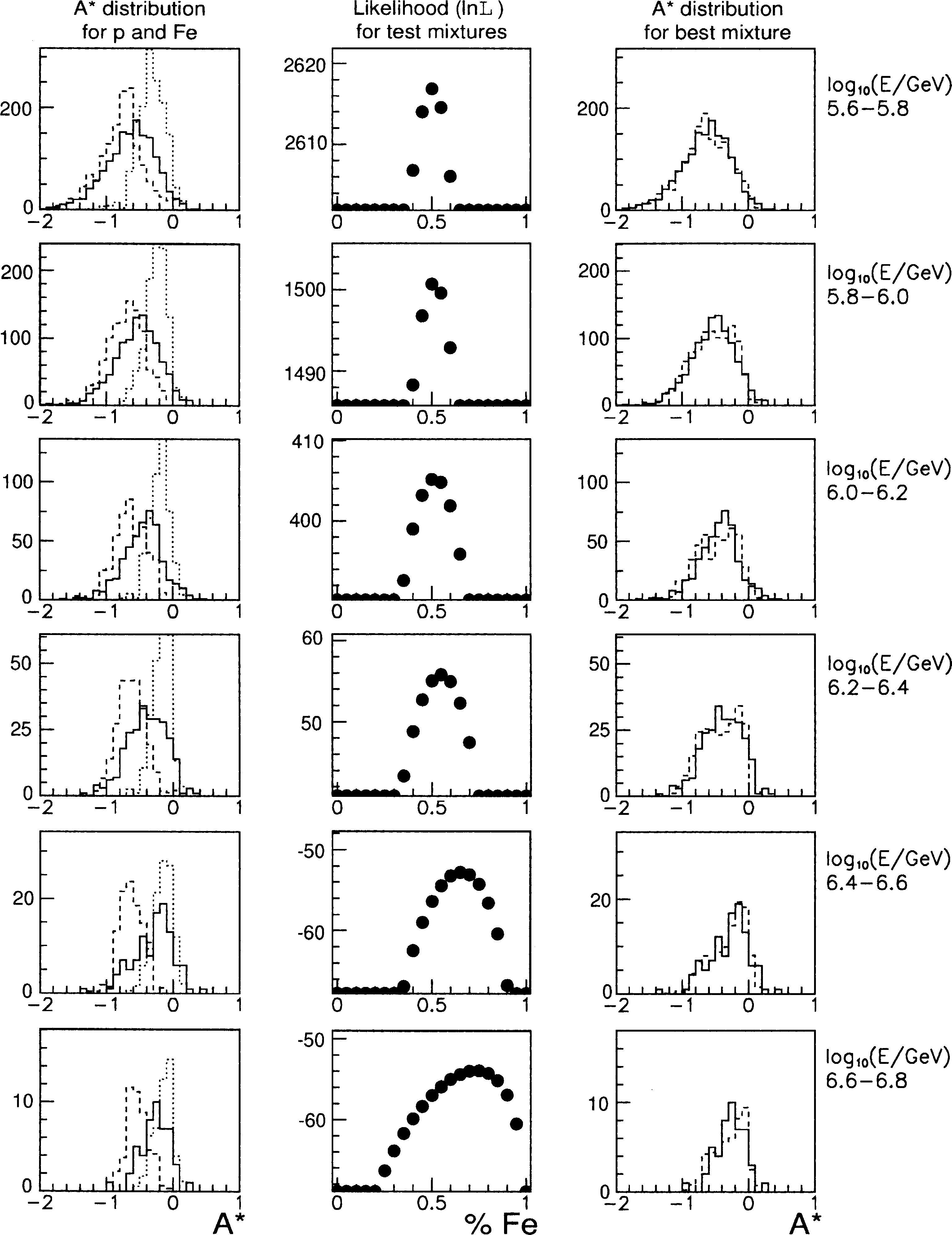
data, so the test compares the histogram shapes.
The Kolmogorov–Smirnov test was also applied to
the histograms as a cross-check, with duplicate
results. The procedure was repeated for each of the
six energy bins; the results for all six bins are
shown in Fig. 11.
6.4. Systematic uncertainties
We are faced with a choice of different shower
generation, muon propagation, and detector
models, each with a different absolute normaliza-
tion. However, calibrating data to Monte Carlo in
a low-energy calibration bin is a technique adapt-
able to any model. By treating each model as an
independent test of normalization and composi-
tion, we can gauge the stability of this technique
under changing models, and estimate the system-
atic error on the final measurement. In addition
to a baseline model, several alternatives can serve
to test the robustness of the analysis to a variation
of parameters. The six models used here are
•
Baseline
. MOCCA/QGSJET, muon propagator
PROPMU, 17-layer ice, 2-component (p and
Fe) composition.
•
Bulk
. Same as baseline, but with uniform ice.
Here we use a simplified ice model which con-
tains no vertical structure.
•
Four component
. p, He, O and Fe nuclei, split
into light and heavy groups with equal weight
within each group.
•
SIBYLL
. The SIBYLL-17 code [24] is used for
the interaction model instead of QGSJET.
•
Amplitude gate
. Here, an incorrect amplitude
readout was used in simulating AMANDA
electronics, resulting in a loss of photon count-
ing accuracy. Using this model tests the sensitiv-
ity of the Monte Carlo to a perturbation in the
electronic response.
•
MMC
. The muon propagator PROPMU has
been replaced with the propagator MMC[25].
For each model, a calibration constant
?
was
computed, and an independent analysis performed
in the same fashion as described above. The same
experimental data were compared to each model in
the variable
A
?
, and the mean log mass and error
bars for the model were computed from the like-
lihood curve. The numerical results from the six
models are summarized in Table 2. While there are
Fig. 10. Sample composition mixtures of p- and Fe-induced showers (dashed), and how they can be compared to data (solid). The
double peak structure in the some mixtures illustrates the separation potential between p and Fe.
576
J. Ahrens et al. / Astroparticle Physics 21 (2004) 565–581
systematic shifts in the
absolute
h
ln
A
i
between
different models, all of the composition measure-
ments follow a similar
trend
.
An additional source of systematic error is
uncertainty in the direct measurement at low
energy, against which the
K
50 parameter is
Fig. 11. For the six constant-energy bins: (left) distributions of
A
?
for pure protons (dashed), pure iron (dotted) and calibrated data
(solid); (middle) ln
ð
L
Þ
as a function of iron percentage and (right) distributions of
A
?
for best mixture of protons and iron (dashed) and
calibrated data (solid). Monte Carlo distributions are normalized to data.
J. Ahrens et al. / Astroparticle Physics 21 (2004) 565–581
577
calibrated and the factor
?
computed. To study
this, a variety of different values of
?
from 0.04 to
0.18 (corresponding to direct measurement
h
ln
A
i
values between 1.8 and 2.2) were tested. The re-
sults are included in the summary, as a distinct
source of error.
7. Results and discussion
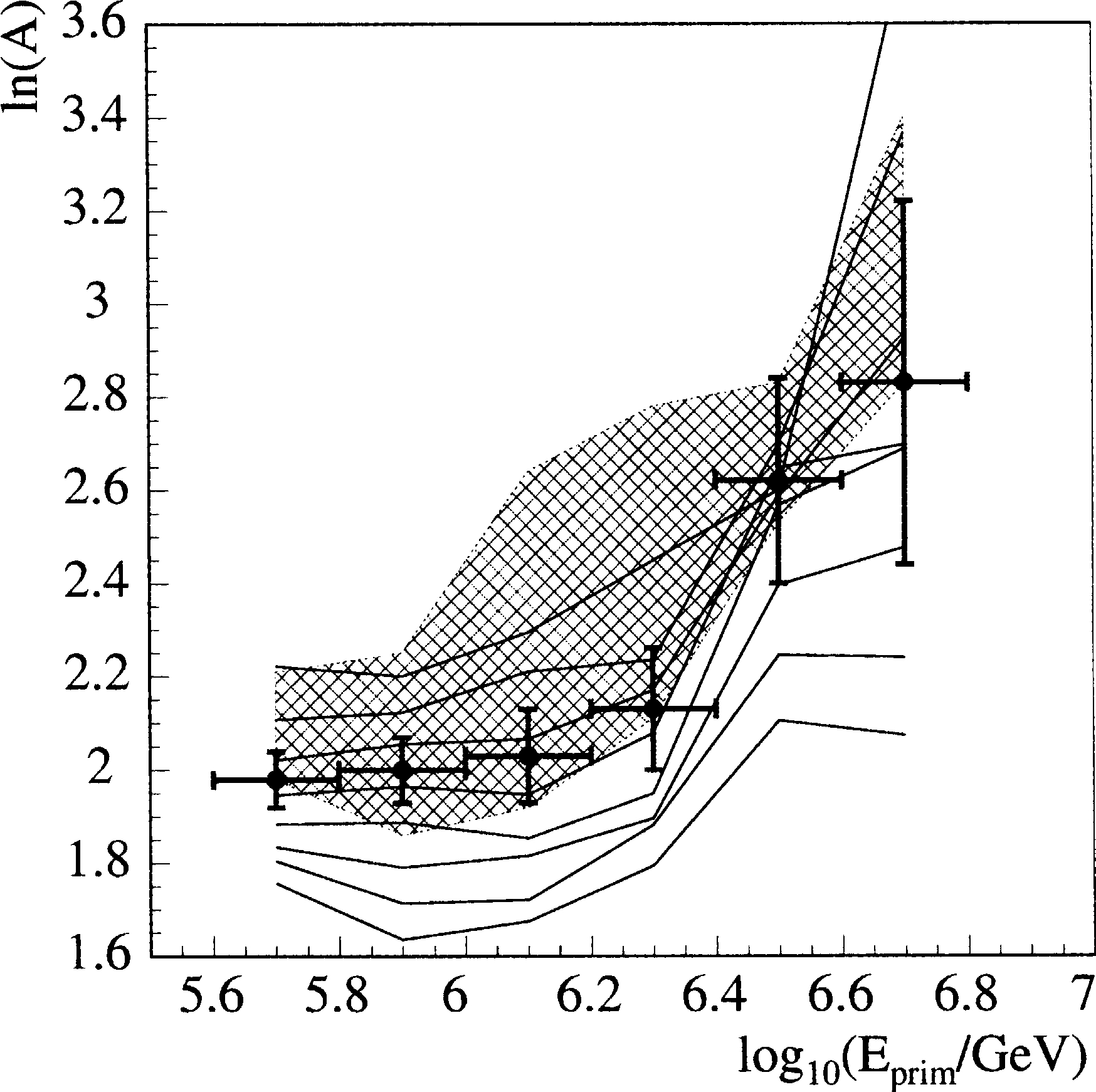
Fig. 12 shows the mean log mass as a function
of the primary energy. Data points indicate the
results from the baseline model, normalized to
h
ln
A
i¼
2
:
0 in the normalization bin, with one
standard deviation statistical error bars computed
from the likelihood curve. The shaded band indi-
cates the range of results obtained using different
simulations, an estimate of the systematic error
from models. Note that these error bars are highly
asymmetric and the baseline model gives values
close to the lower limit. The additional lines indi-
cate results using different initial calibration mix-
tures, corresponding to
?
values from 0.04 to 0.18,
with the baseline simulation, an estimate of the
systematic error from our incomplete knowledge
of
h
ln
A
i
at low energies.
The data show a mass composition consis-
tent with flat between 500 TeV and 1.2 PeV,
after which it starts to become heavier.
h
ln
A
i
in-
creases by 0.9 between 1.2 and 6 PeV. The statis-
tical and systematic errors in the last bins are
too large to allow a good determination of
growth of
h
ln
A
i
. The data are not consistent,
however, with mass becoming lighter through the
knee.
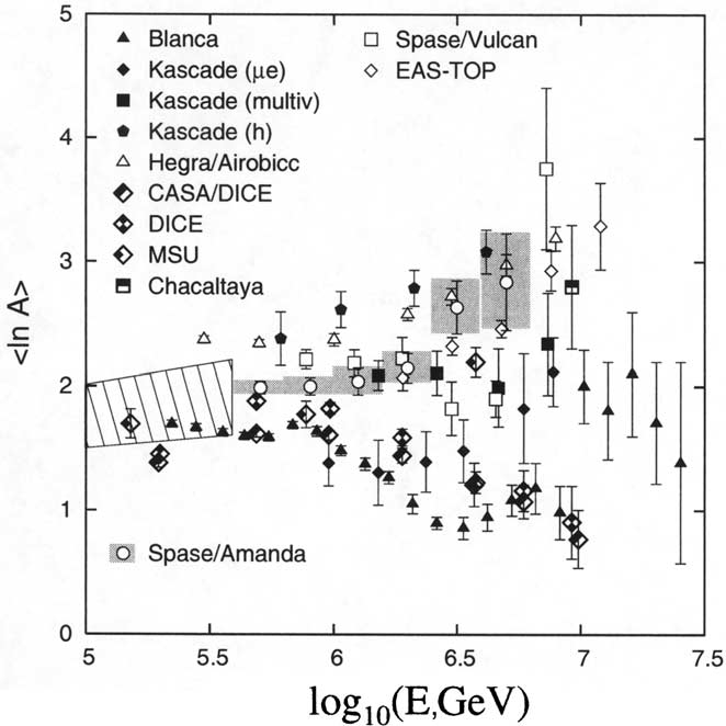
Fig. 13 compares our results with other pub-
lished values obtained with Cherenkov telescopes,
scintillators, and a variety of coincidence experi-
ments. Our results are consistent with most of the
other results that measure cosmic ray composition
becoming heavier with energy. These include the
air shower experiments KASCADE, MSU and
Chacaltaya, the Cherenkov light experiment HE-
GRA/AIROBICC, and the air-shower––deep
Table 2
Summary of composition results from different simulation models
Model Baseline Bulk 4 Comp. SIBYLL Ampl. gate MMC
?
0.14 0.06 0.10 0.01 0.14 0.16
log
10
(
E
/GeV)
h
ln
A
i?
1
r
ð
2
r
Þh
ln
A
i
5.6–5.8 1.98
?
0.06 (0.13) 2.09 1.86 2.08 1.99 2.21
5.8–6.0 2.00
?
0.07 (0.14) 2.05 1.91 1.86 2.00 2.15
6.0–6.2 2.03
?
0.10 (0.21) 2.22 2.42 1.92 2.03 2.36
6.2–6.4 2.13
?
0.13 (0.26) 2.11 2.61 2.13 2.15 2.24
6.4–6.6 2.62
?
0.22 (0.45) 2.53 2.61 * 2.56 2.67
6.6–6.8 2.83
?
0.39 (0.78) 2.87 3.40 * 2.83 3.2
The asterisk indicates omission due to lack of simulated statistics.
Fig. 12. Change of the mass composition relative to the base-
line model as a function of the energy. Error bars represent
statistical 1
r
errors. Shaded region indicates systematic errors
around these center values, defined as the envelope of maximum
deviation in
h
ln
A
i
when using the six perturbations of the
baseline simulation. Additional lines show results using alter-
native values of
?
with the baseline model.
578
J. Ahrens et al. / Astroparticle Physics 21 (2004) 565–581
underground muon telescope EAS-TOP/MACRO.
SPASE/AMANDA result is in conflict only with
the results of BLANCA and DICE (both Cher-
enkov telescopes) which show the mass becoming
lighter in this energy region.
Although each experiment alone has small sta-
tistical error bars (as can be seen in Fig. 13), sys-
tematic errors are often significant and not
displayed in the figure. One can see that many
results do not overlap with each other at low
energies where there is overlap with direct experi-
ments, suggesting differences in systematic errors
between experiments and making them difficult to
compare. Systematic errors are a challenge that all
experiments have in common, which in many cases
dominate the conclusion.
SPASE/AMANDA data indicate an increase of
the mass in the energy range from 1 to 6 PeV and
improve the current knowledge of the mass com-
position in the region of the knee. This result is
significant because the technique and its sources of
systematic error are unique. First, the muon sur-
face energy threshold for detection at depth is
about 300 GeV due to the 1500 to 2000 m of solid
ice overburden above the detector. This is high
enough for sensitivity to the muons created in the
first interactions, yet low enough to overlap with
direct measurements for mass composition cali-
bration. Second, the entire high-energy muon
bundle is measured over a large volume, and the
light output from all muons is sampled over a
track length of 500 m and laterally out to 150 m.
For a PeV iron primary, AMANDA collects a
hundred to several thousand photons over a large
volume, allowing a measurement of the total muon
bundle energy loss. As a result the combined
detectors achieve a mass-independent relative en-
ergy resolution of 0.07 in log
10
(
E
prim
/GeV). This
analysis is also not sensitive to details of the
implementation of the photon propagation, be-
cause
K
50 measures the light intensity at a con-
stant distance from the muon track. The primary
interaction model and the muon propagator are
probed only for the difference between proton- and
iron-induced showers and their energies. Thus, the
method of probing the relative change of muonic
(hadronic) energy to electromagnetic energy in the
air shower is robust and model independent. The
Fig. 13. SPASE/AMANDA composition results compared to other experiments, taken or adapted from [5,10,26–30]. Limits from
direct measurements at low energy are shown as lines.
J. Ahrens et al. / Astroparticle Physics 21 (2004) 565–581
579
location of the SPASE site at high altitude is
advantageous for the electron component, because
the shower maximum is closer to the detector and
fluctuations are not as strong as they are at sea
level.
However, there is room for improvement. Re-
cent data taken with the larger AMANDA-II
array will substantially increase the data statistics.
The rate of coincident events between SPASE-2
and AMANDA-II is increased by a factor of 2–3.
IceCube [31], the next generation neutrino tele-
scope currently in preparation will include a sur-
face array of one square kilometer in size
(
?
10
6
m sr). Simulations indicate that both the size
and technology will be adequate to measure the
mass composition up to 10
18
eV, well beyond any
current result.
Acknowledgements
This research was supported by the following
agencies: National Science Foundation: Office of
Polar Programs, National Science Foundation-
Physics Division, University of Wisconsin Alumni
Research Foundation, Department of Energy, and
National Energy Research Scientific Computing
Center (supported by the Office of Energy Re-
search of the Department of Energy), UC-Irvine
AENEAS Supercomputer Facility, USA; Swedish
Research Council, Swedish Polar Research Secre-
tariat, and Knut and Alice Wallenberg Founda-
tion, Sweden; German Ministry for Education and
Research, Deutsche Forschungsgemein-schaft
(DFG), Germany; Fund for Scientific Research
(FNRS-FWO), Flanders Institute to encourage
scientific and technological research in industry
(IWT), and Belgian Federal Office for Scientific,
Technical and Cultural affairs (OSTC), Belgium;
Particle Physics and Astronomy Research Council,
UK; D.F.C. acknowledges the support of the NSF
CAREER program.
References
[1] J.E. Dickinson et al., Nucl. Instrum. Methods A 440 (2000)
95.
[2] J. Ahrens et al., AMANDA Collaboration, Phys. Rev. D
66 (2002) 012005.
[3] K. Greisen, Progr. Cosm. Ray Phys. 3 (1956) 1.
[4] A. Walker et al., Nucl. Instrum Methods A 301 (1991)
574.
[5] J. Hinton, Ph.D. dissertation, University of Leeds,
1998.
[6] J. Ahrens et al., (AMANDA Collaboration), Muon track
reconstruction and data selection techniques in AMAN-
DA, Nucl. Instrum. Methods A 524 (2004) 169.
[7] M. Aglietta et al., EAS-TOP and MACRO Collaborations,
Phys. Lett. B 337 (1994) 376.
[8] G. Navarra et al., EAS-TOP and LVD Collaborations,
Nucl. Phys. B. Proc. Suppl. 70 (1999) 512.
[9] M. Aglietta et al., EAS-TOP and LVD Collaborations,
Astropart. Phys. 9 (1998) 185.
[10] M. Aglietta et al., Astropart. Phys. 20 (2004) 641.
[11] T. Gaisser, Cosmic Rays and Particle Physics, Cambridge
University Press, 1990.
[12] R.M. Barnett et al., Particle Data Group, Phys. Rev. D 54
(1996) 1.
[13] K. Woschnagg et al., (The AMANDA Collaboration), in:
Proceedings of the of the 26th ICRC, Salt Lake City 2,
1999, p. 200.
[14] K. Woschnagg, private communication.
[15] Y.D. He, P.B. Price, J. Geophys. Res. 103 (1998)
17041.
[16] P. Askebjer et al., Appl. Opt. 36 (1997) 4168.
[17] J. Ahrens et al., (AMANDA and SPASE Collaborations),
Calibration and survey of AMANDA with the
SPASE detectors, Nucl. Instrum. Methods A 522 (2004)
347.
[18] A.M. Hillas, in: Proceedings of the 24th International
Cosmic Ray Conference, Rome, vol. 1, 1995, p. 270.
[19] N.N. Kalmykov, S.S. Ostapchenko, Phys. At. Nucl. 56 (3)
(1993) 346;
N.N. Kalmykov, S.S. Ostapchenko, A.I. Pavlov, Nucl.
Phys. B (Proc. Suppl.) 52B (1997) 17.
[20] P. Lipari, T. Stanev, Phys. Rev. D 44 (1991) 3543.
[21] K. Asakimori (The JACEE Collaboration), in: Pro-
ceedings of the 23rd ICRC (Calgary), vol. 2, 1993, p. 21,
25.
[22] A.V. Apanasenko et al., Astropart. Phys. 16 (2001)
13.
[23] P.R. Bevington, D.K. Robinson, Data Reduction and
Error Analysis for the Physical Sciences, McGraw-Hill,
New York, 1969.
[24] R.S. Fletcher, T.K. Gaisser, P. Lipari, T. Stanev, Phys.
Rev. D 50 (1994) 5710;
J. Engel, T.K. Gaisser, P. Lipari, T. Stanev, Phys. Rev. D
46 (1992) 5013.
[25] W. Rhode, D. Chirkin, in: Proc. of the 27th ICRC
(Hamburg), 2001, p. HE220.
[26] A. Castellina, Nucl. Phys. Proc. Suppl. 97 (2001) 35.
[27] F. Arqueros et al., A&A 359 (2000) 682.
[28] S.P. Swordy et al., Astropart. Phys. 18 (2002) 129–150,
astro-ph/0202159.
580
J. Ahrens et al. / Astroparticle Physics 21 (2004) 565–581
[29] K.-H. Kampert, Invited paper at Vulcano Workshop 2002,
astro-ph/0212348.
[30] A. Haungs, H. Rebel, M. Roth, Rept. Prog. Phys. 66
(2003) 1145.
[31] J. Ahrens et al., The IceCube Proposal to NSF (2000);
J. Ahrens et al., PDD: IceCube Conceptual Design
Document (2001). Available from <http://ice-
cube.wisc.edu>.
J. Ahrens et al. / Astroparticle Physics 21 (2004) 565–581
581
Back to top