Limits to the muon flux from WIMP annihilation in the center of the Earth

with the AMANDA detector

J. Ahrens,

E. Andre

X. Bai,

G. Barouch,

S. W. Barwick,

R. C. Bay,

T. Becka,

K.H. Becker,

D. Bertrand,

A. Biron,

O. Botner,

A. Bouchta,

S. Carius,

A. Chen,

D. Chirkin,

6,11

J. Conrad,

J. Cooley,

C. G. S. Costa,

D. F. Cowen,

E. Dalberg,

2,†

C. De Clercq,

T. DeYoung,

4,‡

P. Desiati,

J.P. Dewulf,

P. Doksus,

J. Edsjo

P. Ekstro

T. Feser,

T. K. Gaisser,

M. Gaug,

8,§

L. Gerhardt,

A. Goldschmidt,

A. Goobar,

A. Hallgren,

F. Halzen,

K. Hanson,

R. Hardtke,

T. Hauschildt,

M. Hellwig,

G. C. Hill,

P. O. Hulth,

S. Hundertmark,

J. Jacobsen,

A. Karle,

J. Kim,

B. Koci,

L. Ko

pke,

M. Kowalski,

J. I. Lamoureux,

H. Leich,

M. Leuthold,

P. Lindahl,

P. Loaiza,

D. M. Lowder,

J. Ludvig,

J. Madsen,

P. Marciniewski,

9,¶

H. S. Matis,

C. P. McParland,

T. C. Miller,

Y. Minaeva,

P. Mioc

inovic

P. C. Mock,

5,††

R. Morse,

T. Neunho

ffer,

P. Niessen,

D. R. Nygren,

H. Ogelman,

Ph. Olbrechts,

C. Pe

rez de los Heros,

9,‡‡

A. Pohl,

R. Porrata,

5,§§

P. B. Price,

G.T. Przybylski,

K. Rawlins,

W. Rhode,

M. Ribordy,

S. Richter,

J. Rodrı

guez Martino,

P. Romenesko,

D. Ross,

H.G. Sander,

T. Schmidt,

D. Schneider,

E. Schneider,

R. Schwarz,

A. Silvestri,

11,8

M. Solarz,

G. M. Spiczak,

C. Spiering,

D. Steele,

P. Steffen,

R. G. Stokstad,

O. Streicher,

P. Sudhoff,

K. H. Sulanke,

I. Taboada,

L. Thollander,

T. Thon,

S. Tilav,

M. Vander Donckt,

C. Walck,

C. Weinheimer,

C. H. Wiebusch,

C. Wiedemann,

R. Wischnewski,

H. Wissing,

K. Woschnagg,

W. Wu,

G. Yodh,

and S. Young

AMANDA Collaboration

Institute of Physics, University of Mainz, D55099 Mainz, Germany

Department of Physics, SCFAB, Stockholm University, S10691 Stockholm, Sweden

Bartol Research Institute, University of Delaware, Newark, Delaware 19716

Department of Physics, University of Wisconsin

–

Madison, Wisconsin 53706

Department of Physics and Astronomy, University of California, Irvine, California 92697

Department of Physics, University of California, Berkeley, California 94720

Universite

Libre de Bruxelles, Science Faculty CP230, B1050 Brussels, Belgium

DESYZeuthen, D15735 Zeuthen, Germany

Division of High Energy Physics, Uppsala University, S75121 Uppsala, Sweden

Department of Technology, Kalmar University, S39182 Kalmar, Sweden

Fachbereich 8 Physik, BUGH Wuppertal, D42097 Wuppertal, Germany

Department of Physics and Astronomy, University of Pennsylvania, Philadelphia, Pennsylvania 19104

Vrije Universiteit, Dienst ELEM, B1050 Brussels, Belgium

Lawrence Berkeley National Laboratory, Berkeley, California 94720

Department of Physics, University of Wisconsin

–

River Falls, Wisconsin 54022

Received 8 February 2002; published 23 August 2002

A search for nearly vertical upgoing muonneutrinos from neutralino annihilations in the center of the Earth

has been performed with the AMANDAB10 neutrino detector. The data collected in 130.1 days of live time

in 1997,

;

events, have been analyzed for this search. No excess over the expected atmospheric neutrino

background has been observed. An upper limit at 90% confidence level has been obtained on the annihilation

rate of neutralinos in the center of the Earth, as well as the corresponding muon flux limit, both as a function

of the neutralino mass in the range 100 GeV–5000 GeV.

DOI: 10.1103/PhysRevD.66.032006 PACS number

: 95.35.

d, 11.30.Pb, 95.30.Cq

Currently at CERN, CH1211, Gene

ve 23, Switzerland.

†

Currently at Defense Research Establishment

FOA

!, S17290 Stockholm, Sweden.

‡

Currently at Santa Cruz Institute for Particle Physics, University of California–Santa Cruz, Santa Cruz, CA 95064.

Currently at IFAE, 08193 Barcelona, Spain.

Currently at MontaVista Software, 1237 E. Arques Ave., Sunnyvale, CA 94085.

Currently at The Svedberg Laboratory, S75121, Uppsala, Sweden.

Currently at Johns Hopkins University, Applied Physics Laboratory, Laurel, MD 20723.

††

Currently at Optical Networks Research, JDS Uniphase, 100 Willowbrook Rd., Freehold, NJ 077282879.

‡‡

Corresponding author. Email: cph@tsl.uu.se

§§

Currently at L174, Lawrence Livermore National Laboratory, 7000 East Ave., Livermore, CA 94550.

PHYSICAL REVIEW D

, 032006

2002

05562821/2002/66

/032006

0320061

I. INTRODUCTION

There are strong observational indications for the exis

tence of dark matter in the universe. Measurements of the

energy density of the universe,

, from the combined

analysis of cosmic microwave background radiation data and

high redshift type Ia supernovae favor

1, with a matter

and a cosmological constant

component. Combined

with data from rotation curves of galaxies and cluster mass

measurements, the matter contribution to

is 0.3

0.4. Big bang nucleosynthesis calculations of primordial

helium, lithium and deuterium production, supported by

abundance measurements of these elements, set an upper

limit on the amount of baryonic matter that can exist in the

universe,

0.05

see Ref.

for a recent review of val

ues of

). Nonbaryonic dark matter must therefore consti

tute a substantial fraction of

In this paper we present results of a search for non

baryonic dark matter in the form of weakly interacting mas

sive particles

WIMP

using the Antartic Muon and Neutrino

Detector Array

AMANDA

highenergy neutrino detector.

Section II contains a brief motivation for WIMPs as dark

matter candidates. Section III describes the characteristics of

the AMANDA detector in the configuration used for this

analysis. Sections IV and V contain a description of the

simulation and analysis techniques used. In Sec. VI we dis

cuss the sources of the current systematic uncertainties of our

analysis. In Sec. VII we present the results of the analysis

and we introduce a novel way of calculating upper limits in

the presence of systematic uncertainties. An upper limit on

the neutrinoinduced muon flux expected from WIMP anni

hilation in the center of the Earth is derived with this

method. A comparison with published muonflux limits ob

tained by existing neutrino experiments is presented in Sec.

VIII.

II. WIMPS AS DARK MATTER CANDIDATES

Particle physics provides an interesting dark matter can

didate as a weakly interacting massive particle

WIMP

. The

relic density of particle type

depends on its annihilation

cross section,

,as

;

neglecting mass

dependent logarithmic corrections

, where

indicates ther

mal average and v is the relative velocity of the particles

involved in the collision

see, for example, Ref.

. Weak

interactions provide the right annihilation cross section for

the WIMPs to decouple in the early universe and give a relic

density within the required range to contribute substantially

to the energy density of the universe today. This is basically

what would be needed to solve the dark matter problem.

In particular, and starting from a completely different ra

tionale, the minimal supersymmetric extension to the stan

dard model of particle physics

MSSM

provides a promis

ing WIMP candidate in the neutralino,

. The neutralino is a

linear combination of the

ino

and the

ino

, the

supersymmetric partners of the electroweak gauge bosons,

and of the H

and H

, the neutral Higgs bosons, and it is

stable

assuming

parity conservation, which is further sup

ported to avoid too rapid proton decay

. The actual compo

sition of the neutralino can have cosmological consequences

since its annihilation cross section depends on it. For ex

ample, it has been argued that a mainly

ino type neu

tralino would not be cosmologically relevant in the present

epoch since it would have annihilated too fast in the early

universe to leave any relevant relic density

Still, the large parameter space of minimal supersymme

try can be exploited to build realistic models which provide

relic neutralino densities within the cosmologically interest

ing region of 0.025

1. Negative results from

searches for supersymmetry at the LEP accelerator at CERN

have set a lower limit on the neutralino mass

31GeV

Ref.

, while theoretical arguments based on the require

ment of unitarity set an upper limit of 340 TeV

Ref.

Imposing in addition the condition on

mentioned

above, only models with

10 TeV

Ref.

become

cosmologically interesting.

Neutralinos have a nonnegligible probability of scatter

ing off nuclei of ordinary matter. Assuming the dark matter

in the Galactic halo is

at least partially

composed of relic

neutralinos, elastic interactions of these particles with nuclei

in the Earth can lead to energy losses that bring the neu

tralino below the escape velocity, becoming gravitationally

trapped

6,7

. For high neutralino masses

greater than a few

hundred GeV

direct capture from the halo population by the

Earth is kinematically suppressed

. In this case neutralinos

can be accreted from the population already captured by the

solar system. Gravitational capture is expected to result in an

accumulation of neutralinos around the core of the Earth,

where they will annihilate. An equilibrium density is reached

when the capture rate equals the annihilation rate. Neutrinos

are produced in the decays of the resulting particles, with an

energy spectrum extending over a wide range of values and

bounded from above by the neutralino mass. Annihilation of

neutralinos directly into neutrinos

or light fermion pairs in

general

is suppressed by a factor

due to helicity

constraints, where

is the fermion mass. Neutrino detectors

can therefore be used to constrain the parameter space of

supersymmetry by setting limits on the flux of neutrinos

from the center of the Earth

2,9

. Note that this indirect

neutralino detection will be favored for high neutralino

masses, since the cross section of the resulting neutrinos with

ordinary matter scales with

III. THE AMANDAB10 DETECTOR

The AMANDAB10 detector consists of an array of 302

optical modules deployed in ten vertical strings at depths

between 1500 m and 2000 m in the South Pole ice cap. The

strings are arranged in two concentric circles of 60 m and

120 m diameter, respectively. The modules on the four inner

strings are separated by 20 m in the vertical direction, while

in the outer six strings the vertical separation between mod

ules is 10 m. An optical module consists of a photomultiplier

tube housed in a spherical glass pressure vessel. Coaxial

cables

in the inner four strings

and twisted quad cables

the outer six strings

provide the high voltage to the photo

multiplier tubes and transmit the signals to the data acquisi

tion electronics at the surface.

J. AHRENS

et al.

PHYSICAL REVIEW D

, 032006

2002

0320062

Muons from chargedcurrent highenergy neutrino inter

actions near the array are detected by the Cherenkov light

they produce when traversing the ice. The relative timing of

the Cherenkov photons reaching the optical modules allows

the reconstruction of the muon track. A more detailed de

scription of the detector is given in Ref.

. The detector

was triggered when a majority requirement was satisfied: an

event was recorded if at least 16 modules had a signal within

a predefined time window of 2

s. The data taking rate was

100 Hz.

AMANDAB10 was in operation during the 1997 Antarc

tic winter. The separation of 300 atmospheric neutrinos from

the data sample collected in that period established the de

tector as a highenergy neutrino telescope

. The array

was upgraded with 122 more modules during the antarctic

summer 1997–1998 and in 1999–2000 253 additional ones

were added, completing the proposed design of 677 optical

modules in 19 strings, AMANDAII

IV. SIGNAL AND BACKGROUND SIMULATIONS

A. Simulation of neutralino annihilations

Neutralinos can annihilate pairwise to, e.g.,

1,2

and

. Neutrinos are

produced in the decays of these annihilation products. Neu

trinos produced in quark jets

from e.g. bb

or Higgs bosons

typically have lower energy than those produced from decays

leptons and gauge bosons. We will refer to the first type

of annihilation channels as ‘‘soft’’ and to the second as

‘‘hard.’’

The simulations of the expected neutralino signal were

done in the framework of the SUSY models described in Ref

. The hadronization and decay of the annihilation prod

ucts have been simulated using

PYTHIA

. The simulations

were performed for six different WIMP masses between 10

GeV and 5000 GeV. For each mass, six different annihilation

channels (

and

) were con

sidered, with 1.25

events generated for each. Note that

the decay of

and

hadrons will take place in matter instead

of vacuum. This was incorporated in the simulations in an

effective manner justified by the fact that, for the neutralino

masses considered, the reinteractions of these heavy hadrons

with the surrounding medium are not dominant, and can be

parametrized as an effective energy loss at the time of decay.

As a reference soft spectrum, we chose the annihilation into

, and as a reference hard spectrum, the annihilation into

. For a given mass, these two spectra can be regarded

as extreme cases. We have used these channels in the analy

sis described below, bearing in mind that a typical spectrum

would lie somewhere in between.

B. Simulation of the atmospheric neutrino flux

Neutrinos from the decay of secondaries produced in cos

mic ray interactions in the atmosphere constitute the physical

background to the neutralino search. We have simulated this

atmospheric neutrino flux using the calculations of Lipari

. To obtain the rate of neutrino interactions producing

muons we have used the neutrino and antineutrino–nucleon

cross sections from Gandhi

et al.

. The actual neutrino

nucleon interactions have been simulated with

PYTHIA using

the

CTEQ3

parametrization of the nucleon structure func

tions. The use of

PYTHIA

allows to model the hadronic

shower produced at the vertex of the interaction and, there

fore, to calculate the Cherenkov light produced by secondar

ies. When the neutrinonucleon interaction occurs within the

instrumented volume of the detector, this is a nonnegligible

contribution to the total event light output.

A threeyear equivalent atmospheric neutrino sample with

energies between 10 GeV and 10 TeV and zenith angles be

tween 90°

horizontal

and 180°

vertically upgoing

has

been simulated

. The sample contains 3.7

events, of

which 41234 triggered the detector.

C. Simulation of the atmospheric muon flux

The majority of the triggers in AMANDA are induced by

muons produced in cosmic ray interactions in the atmosphere

and reaching the detector depth. The simulation of this atmo

spheric muon flux was performed using the

BASIEV

pro

gram. We note that this program only uses protons as prima

ries. However, the systematic uncertainty introduced by this

approximation is negligible in comparison with that from the

present uncertainty in the primary flux intensity. Moreover,

heavier nuclear primaries produce more muons per interac

tion, but with lower energies on average

, which will in

general loose all their energy and decay before reaching the

detector. A study performed using the

CORSIKA

air

shower generator, with the

QGSJET option to model the had

ronic interactions, including the complete cosmic ray com

position confirms this scenario.

The simulation of a statistically significant sample of at

mospheric muon background is an extremely high CPUtime

consuming task due to the strong rejection factors needed.

We have simulated 6.3

primary interactions, distrib

uted isotropically with zenith angles,

, between 0 and 85

degrees, and with energies,

, between 1.3 TeV and 1000

TeV, assuming a differential energy distribution

}

2.7

Ref.

. The total number of triggers produced were 5

Normalizing to the primary cosmic ray rate, the generated

sample corresponds to about 0.6 days of equivalent detector

livetime. Due to the narrow vertical angular cones used for

this analysis this background sample is sufficient to model

the detector response and develop the rejection cuts. In ad

dition, a larger sample of background data was used in the

training of the discriminant analysis program used as cut

level 4. This is described in more detail in the next section.

D. Muon propagation

The muons produced in the signal and background simu

lations described above were propagated from the production

point to the detector taking into account energy losses by

bremsstrahlung, pair production, photonuclear interactions

and

ray production from Ref.

. The Cherenkov light

emitted by the secondaries produced in these processes is

taken into account when calculating the response of the de

tector to the passage of the muon.

LIMITS TO THE MUON FLUX FROM WIMP... PHYSICAL REVIEW D

, 032006

2002

0320063

V. DATA ANALYSIS

The analysis presented in this paper was performed on

data taken with the 10string AMANDA detector between

March and November 1997. The experimental data set con

sists of 1.05

events in a total of 130.1 days of detector

livetime. The data were first cleaned of noise hits and hits

from optical modules that were unstable during the running

period. Short pulses that are likely induced by cross talk

between channels are also rejected at this stage. Details on

the data cleaning procedure are given in Ref.

. The data

are then reconstructed and five filters consisting of cuts based

on the event hit pattern and the quality of the reconstruction

are applied in order to identify potential upgoing neutrino

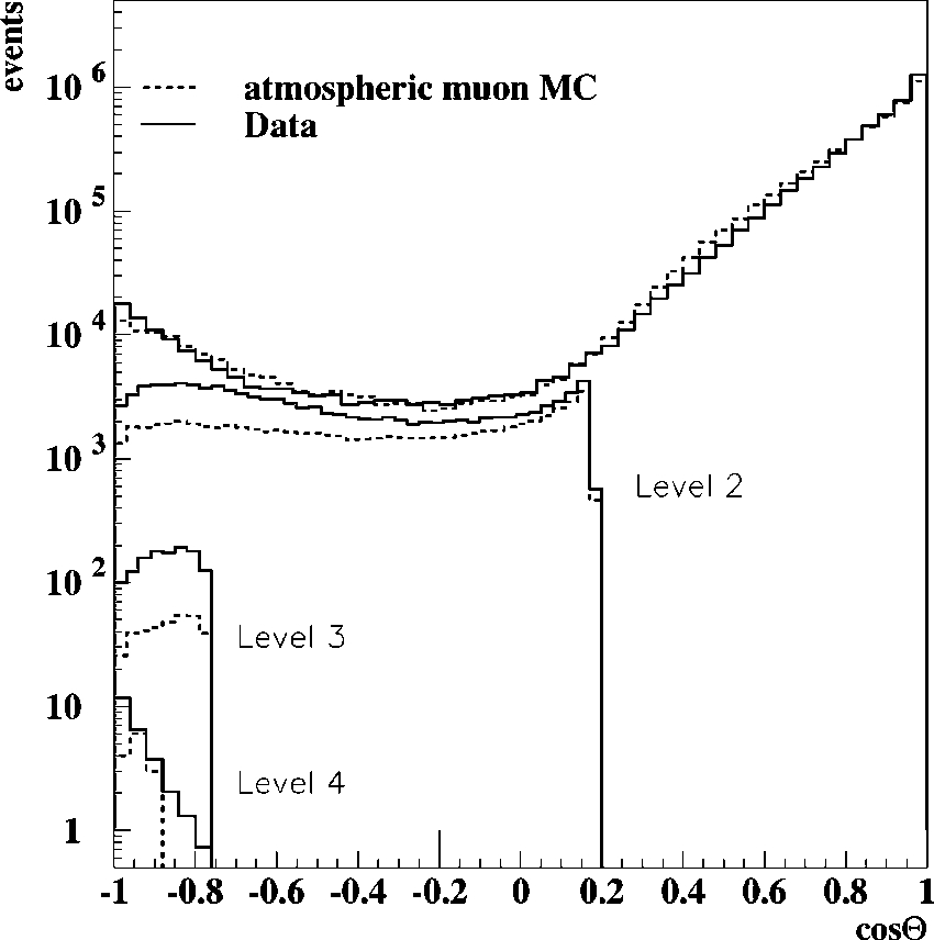
candidates. The distributions of the reconstructed zenith

angle from trigger level

after hit cleaning

until filter level 4

for data and simulated atmospheric muons are shown in Fig.

1. The curves have been normalized to the simulated sample,

events. The uppermost curves in the plot show the

reconstructed direction without any quality criteria applied to

the fits, showing good agreement between the data and the

Monte Carlo sample along the whole angular range. The

curves clearly indicate that a small percentage

about 2%

the originally downgoing tracks are misreconstructed as up

going (cos

less than zero the figure

. The series of cuts

described below were developed to reject such misrecon

structions, and their effect on the angular distribution is also

shown in Fig. 1 for comparison. The filter level 2 and level 3

curves show that the filtering procedure is more effective

rejecting the simulated muon background than the data. This

is due to detector effects not included in the simulation of the

detector response and surviving to these levels, like elec

tronic cross talk between channels or inefficiencies of the

digitizing electronics. Other processes not included in the

background simulations that can contribute to the discrep

ancy are overlapping events from uncorrelated cosmic ray

interactions and the contribution from electron neutrino in

duced cascades. To account for this different behavior be

tween data and simulated background under standard cuts,

we have used an iterative discriminant analysis as cut level 4

see Sec. V D

trained on a subsample of data

which rep

resents the real remaining background better than the simu

lations

and a subsample of the neutralino signal. A final

series of high quality cuts were applied after the discriminant

analysis, bringing the remaining data sample to agree with

the number of events expected from the known atmospheric

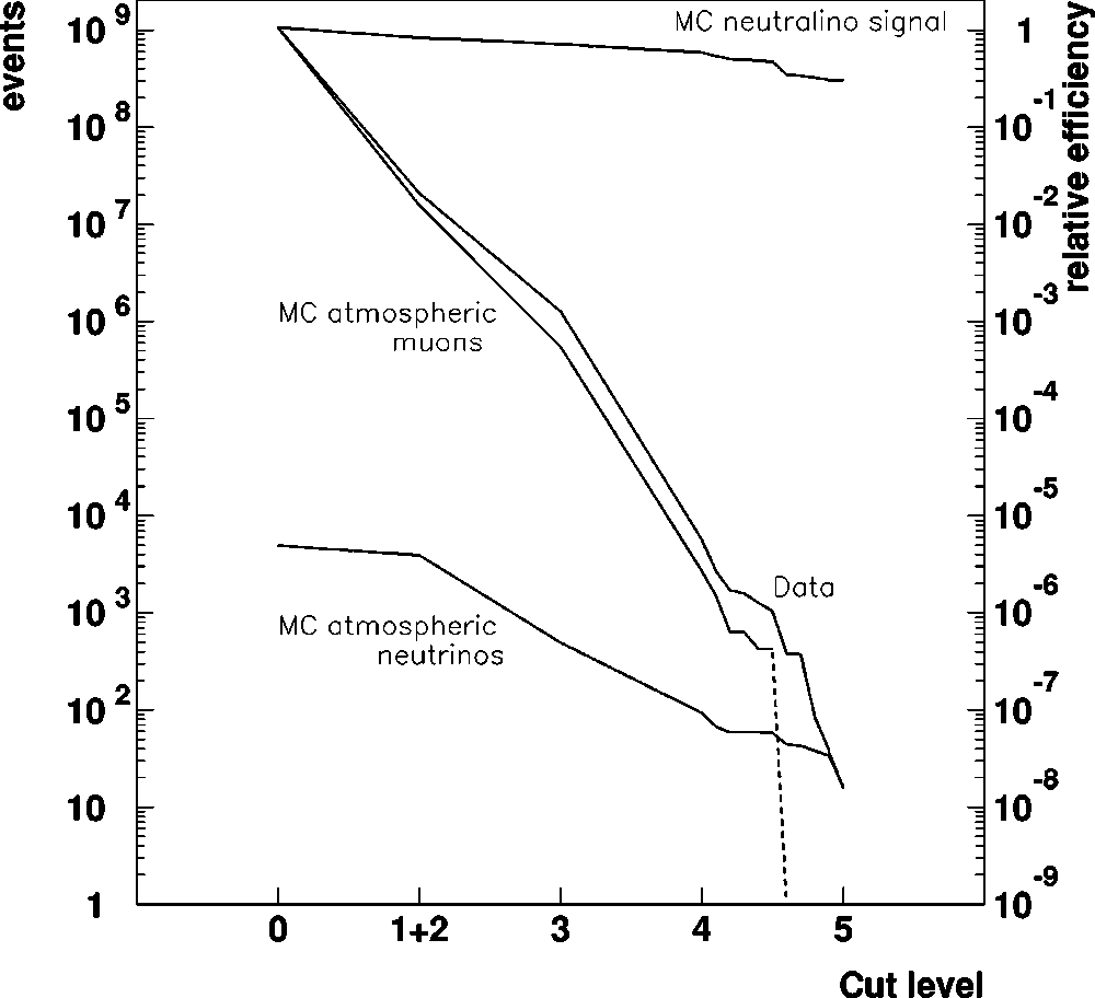
neutrino flux, as shown in Fig. 2 and Table I. Note that the

atmospheric neutrino curve and the data curve in Fig. 2 join

and follow each other in the last two steps of the cuts applied

within the level 5 filter. The following subsections give a

more detailed description of the variables used and the cuts

applied at each filter level.

A. Filter level 1

In a first stage, a simple and computationally fast filter

based on fitting a line to the time pattern of the events was

applied to the data sample in order to reject obvious down

going tracks. This ‘‘line fit’’

assumes that the known

space point of each hit optical module,

, is related to the

measured hit time,

,by

. The minimization of

(

)

, where the index runs over all the hits

in the event, leads to an explicit solution for

. The zenith

angle of the fitted track is readily obtained as cos

. The angular resolution of the line fit is relatively

low since it does not incorporate any information about the

FIG. 1. Angular distributions of data and atmospheric muon

simulation Monte Carlo

at different analysis levels. Top to

bottom: trigger to level 4. The distributions are normalized to the

simulated sample, 5

events.

FIG. 2. Rejection and efficiency at each filter level for the data

and simulations of the neutralino signal, atmospheric neutrinos and

atmospheric muons. The dashed part corresponds to rejection levels

surpassing the statistical precision of the simulated sample, yielding

zero remaining events. The neutralino signal curve should be read

only with respect to the right axis scale, and it shows the relative

signal efficiency with respect to trigger level. The rest of the curves

are plotted with respect to the left axis scale.

J. AHRENS

et al.

PHYSICAL REVIEW D

, 032006

2002

0320064

geometry of the Cherenkov cone or about scattering of the

Cherenkov photons in the ice. Still, its simplicity and com

putational speed makes it a very useful tool for a first assess

ment of the track direction and for rejection of downgoing

atmospheric muons

. The first level filter rejected obvi

ous downgoing atmospheric muons by requiring

50°.

B. Filter level 2

The events that pass the level 1 filter are reconstructed

using a maximum likelihood approach

as described in

. In short, the ML technique uses an iterative process to

maximize the product of the probabilities that the optical

modules receive a signal at the measured times, with the

track direction

zenith and azimuth angles

as free param

eters. The expected time probability distributions include the

scattering and absorption characteristics of the ice as well as

the distance and relative orientation of the optical module

with respect to the track

The level 2 filter consists of two cuts: the ML

reconstructed zenith angle must be larger than 80° and at

least three hits must be ‘‘direct.’’ A hit is defined as direct if

the time residual,

res

the difference between the measured

time and the expected time assuming the photon was emitted

from the reconstructed track and did not suffer any scatter

ing

, is small. Unscattered photons preserve the timing infor

mation. Therefore, the reconstruction of the direction of

tracks with several direct hits presents a significantly better

angular resolution. The number of direct hits associated with

a track is the first quality requirement applied to the recon

structed data and simulated samples

. A residual time

interval between

10 ns and 25 ns was used to classify a hit

as direct at this level.

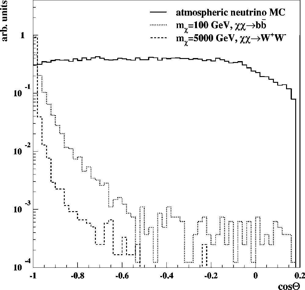
Figure 3 shows the zenith angle distributions of simulated

muon tracks from neutrinos produced in annihilation of neu

tralinos for the two extreme masses used in this analysis as

compared to that from atmospheric neutrinos after filter level

2. The corresponding curve for data and simulated atmo

spheric muons is included in Fig. 1. The combined effect of

these two filters on the data is a rejection of 98%, as shown

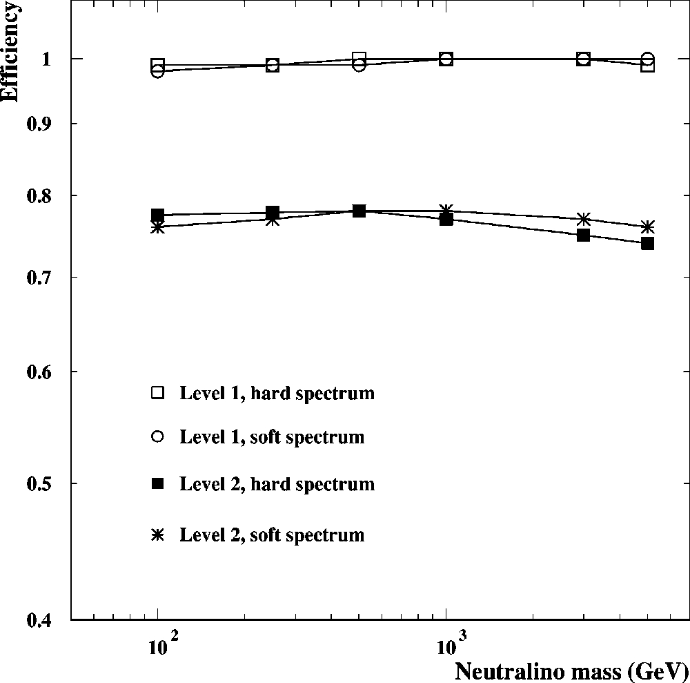
in Table I. The efficiencies with respect to trigger level of

both level 1 and level 2 filters for simulated neutralino signal

are shown in Fig. 4, for different neutralino masses and the

two extreme annihilation channels used.

Filters 1 and 2 are applied in an initial data reduction

common to the different subsequent analyses of the data. The

rest of the cuts described below were specifically designed

for the WIMP search with the aim of identifying and reject

ing misreconstructions while maximizing signal detection ef

ficiency and background rejection

C. Filter level 3

The angular distribution of the events is the most obvious

difference between the predicted neutralino signal and both

the atmospheric neutrino flux and the atmospheric muon

background. Neutrinos from neutralino annihilations in the

center of the Earth would be concentrated in a narrow cone

close to the vertical direction, while atmospheric neutrinos

are distributed isotropically. The level 3 filter further re

stricted the MLreconstructed zenith angle to be larger than

140°, placed a cut on the total number of hit modules in the

event, N

10, and on the summed hit probability of the

modules with a signal, P

hit

0.23. The number of hits with

time residuals between

10 ns and 25 ns was required to be

larger than 4 and the number of hits with residuals between

TABLE I. Rejection of data, of the simulated atmospheric neutrinos and of the atmosphericmuon back

ground samples and efficiency for the simulated neutralino signal from trigger level to filter level 5.

Filter level Data Atmospheric neutrinos Atmospheric muons

130.1 days 130.1 days equivalent 0.6 day equivalent

250 GeV

events

% of trigger level

0 1.05

4899 5

100

2 2.3

2606 7

3 1.2

472 2588 68

4 5441 89 13 56

5 14 16.0 0 29

FIG. 3. Angular distribution of muons from atmospheric neutri

nos and from the annihilation of neutralinos after filter level 2. The

two extreme neutralino masses and annihilation channels consid

ered in this paper are shown. The relative normalization is arbitrary.

LIMITS TO THE MUON FLUX FROM WIMP... PHYSICAL REVIEW D

, 032006

2002

0320065

15 ns and 75 ns to be larger than 5. At this stage the

possible correlations between the variables are ignored, and

the cuts applied to each of them individually. Table I shows

the efficiency and rejection power at this cut level. Only 5

of the simulated atmospheric muon background sur

vive this level, compared with 68% of the simulated neu

tralino signal and 10% of the atmospheric neutrinos.

D. Filter level 4: iterative discriminant analysis

To account for possible correlations between the variables

and to perform a multidimensional cut in parameter space,

the next filter level was based on an iterative nonlinear dis

criminant analysis, using the IDA program

. Given a set

variables, the program builds the ‘‘event vector’’

(

, ...,

), where

is the value of variable

in event

. A class of events, the

signal or background sample, is characterized by their mean

vector

, and the mean difference between the

samples is given by the vector

. The spread

of the variables is contained in the variance vectors,

and

, which are used to define a

variance matrix for each class,

(

)

where

is the number of events in the signal or back

ground samples and T denotes the transpose. The problem of

separating signal from background is transformed into the

problem of finding a hyperplane in event vector space which

gives minimum local variance for each class and maximum

separation between classes. This is translated into the re

quirement that the ratio

(

)

should be maxi

mal, where here the variance matrix

is the sum of the

variance matrices for signal and background and

is a vector

of coefficients to be determined by training the program on a

signal and a background sample. A target signal efficiency

and background rejection factor are chosen beforehand. The

coefficients

are determined in an iterative process carried

out until the specified rejection factor is achieved or a pre

defined number of iterations reached. The coefficients found

in this way are used to select events from the signal region in

the multidimensional parameter space: each event is charac

terized by the scalar

and a cut on

serves as the

selection criterion.

Eight variables were used in the training of the discrimi

nant analysis program and in the subsequent cuts: the veloc

ity of the line fit, the number of direct hits, the number of

modules hit, the number of modules hit in the string with the

largest number of hits, the number of detector layers with a

hit,

the extension of the event along the three coordinate

axes, the average hit probability and the probability that the

event time pattern is compatible with that expected from a

vertical upgoing muon. This set of variables includes com

bined information from the fit track parameters as well as the

general spatial and temporal topology of the event.

Since to a first approximation the data consist of atmo

spheric muon background, seven days of data, evenly distrib

uted along the year, were used as the background training

sample. For the signal training sample, muons from the

simulations of 250 GeV neutralinos annihilating into a hard

spectrum were used. The combination of a relatively low

neutralino mass and annihilation into the hard channel was

chosen as giving a ‘‘typical’’ muon spectrum. The target sig

nal efficiency was set to 98% per iteration and the target

global background rejection to 1000. The stopping criterion

was set to 9 iterations, based on the fact that further loops

would reduce the number of events in the training sample to

a too low number to be representative of the whole data set.

The rejection of background achieved was 220 with respect

to cut level 3 since the nine loops were exhausted before

reaching the desired rejection. The overall signal efficiency

attainable after the training process is then (0.98)

0.83.

The effect of the discriminant analysis event selection is

shown in Table I. It indeed achieves the expected signal ef

ficiency, retaining 82% of the signal with respect to the pre

vious cut level. The discrepancy of the expected number of

atmospheric neutrinos and the number of remaining data

events at this level indicates that the data sample is still con

taminated by poorly reconstructed downgoing muons. A last

cut level was therefore developed to improve the rejection of

the remaining misreconstructed events and select the truly

upgoing tracks.

E. Filter level 5: final event selection

The remaining events after the discriminant analysis with

a zenith angle larger than 165° were passed through the fol

lowing series of cuts. The length spanned by the direct hits

when projected along the track direction was required to be

at least 110 m, and the vertical length containing all hits was

required to be at least 170 m. The

component of the center

The detector was divided in eight horizontal layers of 65 m

depth.

FIG. 4. Efficiencies relative to trigger level at filter levels 1 and

2 as a function of the neutralino mass.

J. AHRENS

et al.

PHYSICAL REVIEW D

, 032006

2002

0320066

of gravity of the direct hits (

c.o.g.

(

direct hits

, where the

sum is over all the direct hits in the event

was required to be

deeper than 1590 m, and the percentage of hits in the lower

half of the detector less than 55%. These cuts reject events

with a spatially uneven concentration of hits, typically due to

downgoing atmospheric muons that pass just outside the

detector or stop close to the array.

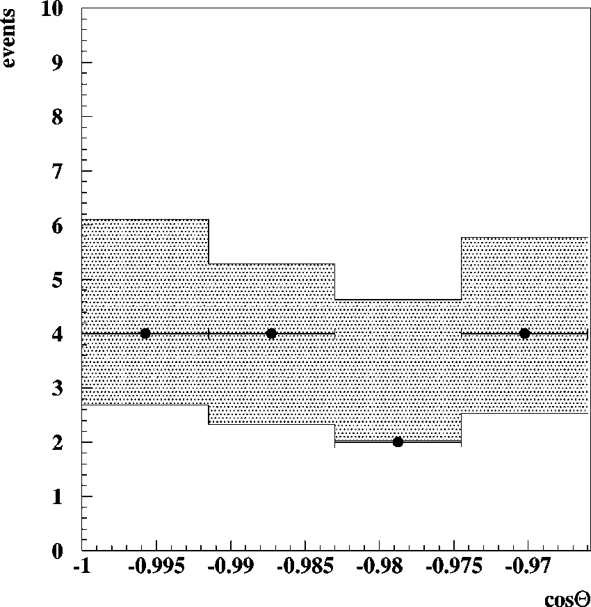
The remaining data at this level are consistent with the

expected atmospheric neutrino flux. Figure 5 shows the an

gular distribution of the remaining 14 data events and the

remaining 16.0 simulated atmospheric neutrino events. The

angular range shown is for

165°, the region where a

possible neutralino signal is expected to be concentrated. No

statistically significant discrepancies are found between the

expected number of events and angular distributions of the

atmospheric neutrino background and the data. This result is

also consistent with the results on atmospheric neutrinos pre

sented in Ref.

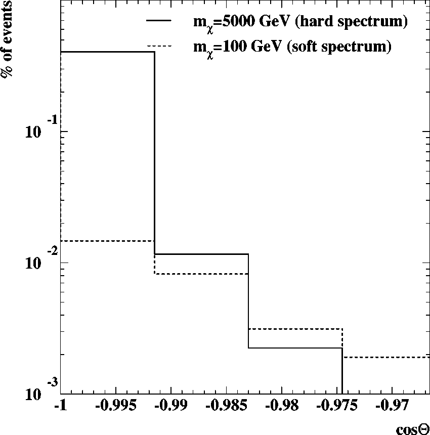
Due to the different angular shapes of the neutralino sig

nal for different neutralino masses

see Fig. 6 for the two

extreme cases considered

, we have chosen to restrict further

in angle the signal region we use to extract the limit on an

excess muon flux. We use angular cones that contain 90% of

the signal for a given neutralino mass. The remaining data

and simulated atmospheric neutrino background events for

the different angular cones used are shown in Table II. The

background rejection power and signal efficiency from filter

level 1 to 5 are shown in Fig. 2 along with the effect on the

data sample.

VI. SYSTEMATIC UNCERTAINTIES

An essential quantity when deriving limits, as we do in

the next section, is the effective volume,

eff

, of the detector.

It is the measure of the efficiency to a given signal and it is

defined as

eff

gen

where

is the number of signal events after filter level 5

and

gen

the number of events simulated in a volume

gen

FIG. 5. Angular distribution of the remaining data events

dots

and simulated atmospheric neutrino events

shaded area

at filter

level 5. The angular range shown is between 165° and 180°. The

shaded area represents the total uncertainty in the expected number

of events.

FIG. 6. Angular distribution of the remaining fraction of neu

tralinos at filter level 5 with respect to the trigger level from the two

extreme neutralino masses studied in this paper. The angular range

shown is between 165° and 180°.

TABLE II. Number of data events, simulated atmospheric neu

trino background events and the corresponding

for the angular

cones containing 90% of the signal for the different neutralino

masses. These angular cuts are applied in addition to the level 5

filter described in Sec. V. ‘‘s’’ and ‘‘h’’ denote the soft and hard

annihilation channels. The numbers in parentheses in column 5

show

obtained without including systematic uncertainties.

Angular cut Data Atmospheric

GeV

deg

events

neutrinos

events

100s 167.5 10 12.1 9.2

4.7

100h 168.5 9 10.8 6.6

4.7

250s 170.0 7 8.6 5.9

4.1

250h

500s

172.0 5 6.1 5.6

3.9

1000s 173.0 4 4.6 5.3

3.9

500h 173.5 4 4.6 5.3

3.9

1000

3000

174.0 4 3.9 5.6

4.7

3000

5000

174.5 3 3.9 4.4

3.6

LIMITS TO THE MUON FLUX FROM WIMP... PHYSICAL REVIEW D

, 032006

2002

0320067

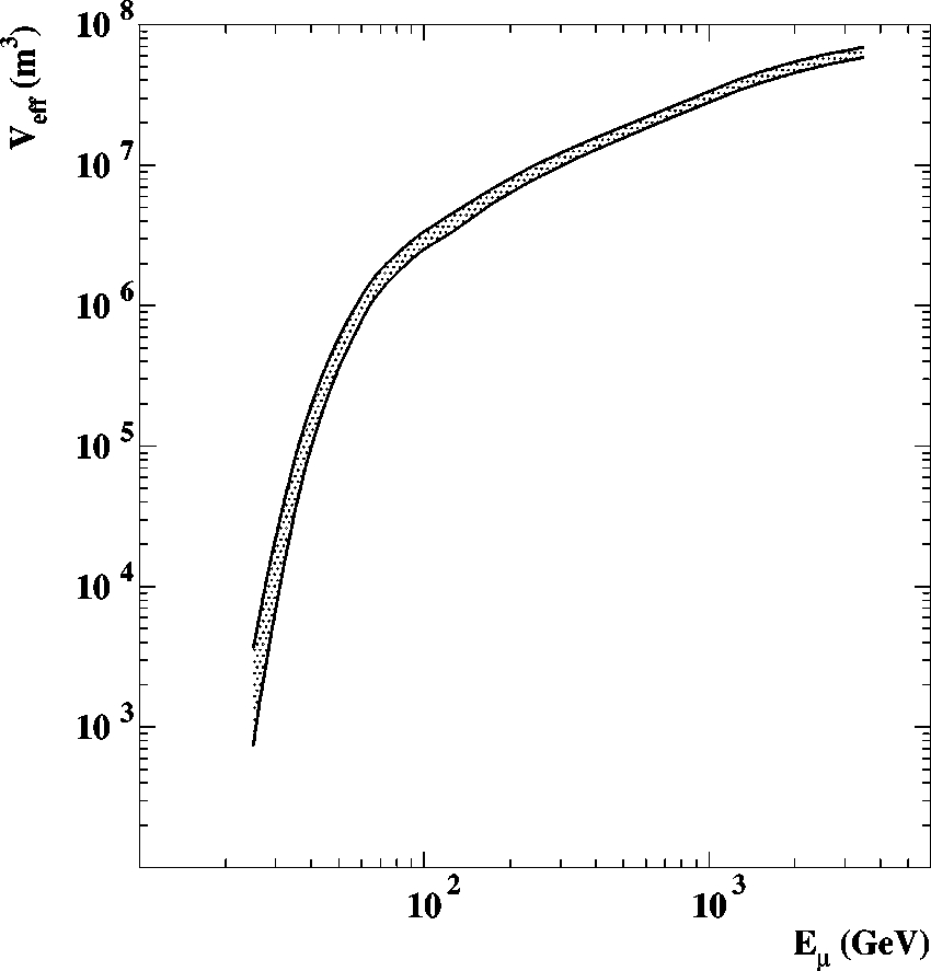
surrounding the detector. The effective volume of

AMANDAB10 as a function of muon energy is shown in

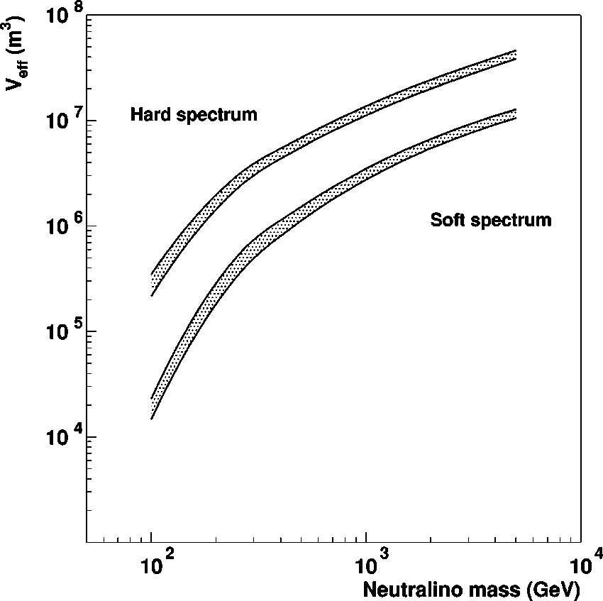
Fig. 7. Given a MSSM model producing a muon flux with a

given muon energy spectrum, the effective volume of the

detector for this particular signal is also calculated through

Eq.

. This is shown in Fig. 8 for the different neutralino

masses used in this analysis. The shaded bands in both fig

ures indicate the systematic uncertainty estimated as de

scribed below.

The evaluation of

eff

is subject to experimental and the

oretical systematic uncertainties present in the analysis. We

have performed a detailed study of the effect of the uncer

tainty in several variables on the resulting effective volume

by propagating variations in any of them to the final evalu

ation of

eff

Measurements of the scattering and absorption lengths,

and

, using pulsed and DC light sources deployed with the

detector at different depths and light from an yttrium alumi

num garnet

YAG

laser sent from the surface through opti

cal fibers, have shown that these quantities exhibit a depth

dependence which is correlated with dust concentration at

different levels in the ice

. A simulation of the detector

response, including layers of ice with different optical prop

erties, has been developed and used to evaluate its effect on

the results. The effects introduced are muonenergy depen

dent and therefore dependent on the neutralino model. The

effective volumes calculated with the layered ice model are

reduced between 1% and 20% with respect to the uniform

ice model, except for the lower neutralino mass and soft

annihilation channel

100 GeV

where the effect reaches

50%.

A further correction accounts for the uncertainties in the

optical modules’ total and angular sensitivities. It is known

that during the process of refreezing after deployment, air

bubbles appear in the column of ice that has been melted,

changing locally the scattering length of the ice and distort

ing the effective optical module angular sensitivity with re

spect to that measured in the laboratory. We have used a

specific ice model for the ice in the holes that accommodates

this effect. The fact that it appears after deployment and that

it is not directly measurable in the laboratory makes it diffi

cult to assess. Only by an iterative process of comparison of

data and different holeice models can it be quantified. We

estimate this effect to yield and increase of 20% in effective

volume with respect to the uniform angular response model

with, again, the soft annihilation channel of the lowest mass

neutralino giving a stronger effect of 34%. An additional

20% uncertainty on the total optical module sensitivity has

been used.

The way to combine all these effects into a final estimate

of the total uncertainty in

eff

is a difficult subject, since they

are not independent contributions. As described in the previ

ous paragraphs, by varying the initial parameters used in the

simulations of the detector and in the ice properties, we have

obtained a range of possible values for the effective volume,

which we consider as equally probable giving our current

understanding of the detector. We have chosen to take the

nominal

eff

to be used in Eq.

as the middle value of this

range. As a conservative estimate of the uncertainty we take

half the width of the range of values obtained. We thus con

clude that our current estimate of

eff

is affected by a sys

tematic uncertainty

eff

between 10% and 25%, de

pending on the neutralino mass considered, the lower mass

of 100 GeV giving the larger relative error. A similar esti

mate including the same effects has been made for the atmo

spheric neutrino Monte Carlo. In this case we estimate the

uncertainty on the effective volume for atmospheric neutri

nos to be 20%.

Further uncertainty in the number of expected atmo

spheric neutrinos

column 3 in Table I

is caused by the

uncertainties present in the calculation of the atmospheric

neutrino flux. This is estimated to be of the order of 30% in

the energy region relevant to this analysis, and originates

mainly from uncertainties in the normalization of the pri

FIG. 7. Effective volume of the detector as a function of muon

energy at filter level 5.

FIG. 8. Effective volumes for the neutralino signal as a function

of the neutralino mass.

J. AHRENS

et al.

PHYSICAL REVIEW D

, 032006

2002

0320068

mary cosmic ray spectrum and in the hadronic cross sections

involved

. This has been taken into account as an addi

tional effect on top of the experimental uncertainty on the

effective volume for atmospheric neutrinos, as described in

Sec. VII B.

It has recently been shown that different muon propaga

tion codes can produce differences in the muon flux and

energy spectrum at the detector depth

see, for example, Ref.

. The code used in this analysis uses the Lohmann

parametrizations for muon energy loss, which produce re

sults in agreement within about 10% of more recent codes

for muon energies up to a few of TeV. We have not

included any systematics arising from the treatment of muon

propagation in the ice in this analysis.

VII. RESULTS

From the observed number of events,

obs

, and the num

ber of expected atmospheric neutrino background events,

, an upper limit on the signal,

, at a chosen confidence

level

%, can be obtained. We have used the unified ap

proach for confidence belt construction

to calculate 90%

confidence level limits. In Sec. VII B below we briefly de

scribe a novel way of calculating limits in the presence of

systematic uncertainties that we have used to obtain the final

numbers presented in this paper.

A. Flux limits: the standard approach

For detectors with a fixed geometrical area

, it is natural

to derive a muon flux limit directly through

where

is the detector livetime. However, due to the large

volume of AMANDA and the lack of sharp geometrical

boundaries it is the effective volume

eff

, as defined in Eq.

, that has to be used to determine a limit on the volumetric

neutrinotomuon conversion rate,

. The effective vol

ume provides a measure of the detector efficiency since, in

addition to throughgoing tracks, it takes into account the

effect of tracks starting or stopping within the detector. A

limit can then be set on

, that is, on the number of muons

with an energy above the detector threshold

thr

produced by

neutrino interactions per unit volume and time,

eff

includes all the detector threshold effects and model

dependencies, as indicated below, and can be directly related

to a more physically meaningful quantity, the annihilation

rate,

, of neutralinos in the center of the Earth through

(

...

thr

where the term inside the integral takes into account the pro

duction of muons through the neutrinonucleon cross section,

, weighted by the different branching ratios of the

annihilation process and the corresponding neutrino energy

spectra,

is the nucleon density of the

ice and

is the radius of the Earth. We have used a muon

energy threshold of 10 GeV in the simulations of the signal,

which has been taken into account through the muon produc

tion cross section.

Equation

is solved for

depends on the MSSM

model assumptions, as well as the galactic halo model used,

being related to the capture rate of neutralinos in the Earth.

Different neutralino models predict different capture and an

nihilation rates that can be probed by experimental limits set

. The right column of Table III shows the limits thus

derived for

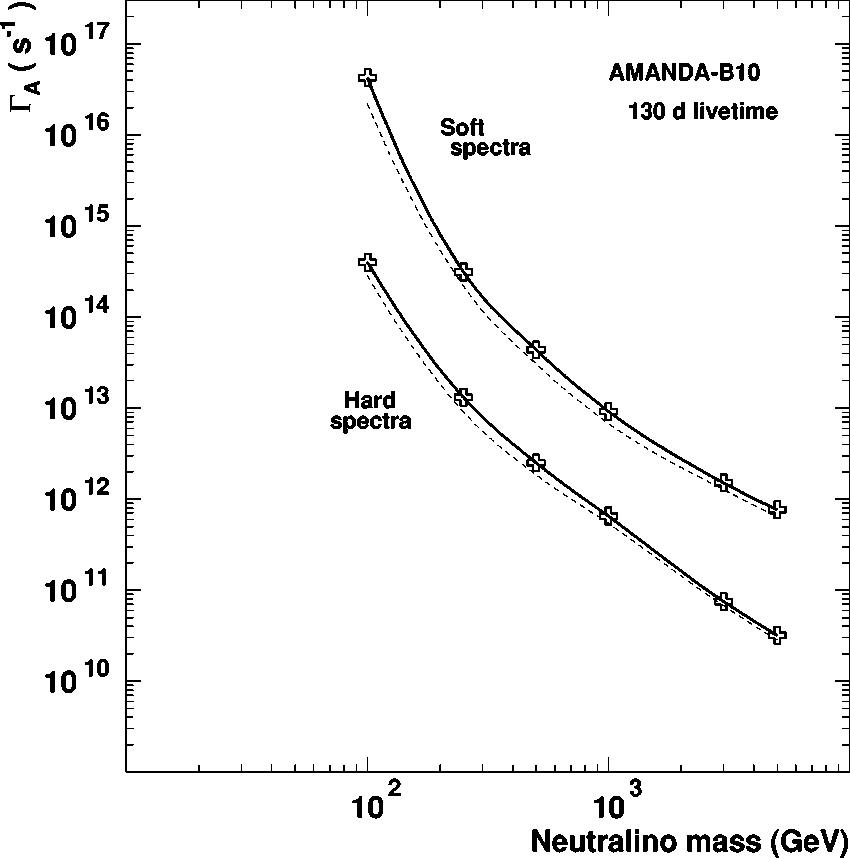
. The corresponding curves are shown in Fig.

9. Quoting limits on the annihilation rate has the advantage

that the detector efficiency and threshold are included

through Eq.

and, therefore, numbers published by differ

ent experiments are directly comparable. This is not usually

the case when presenting limits on muon fluxes, where at

least the detector energy threshold enters in a nontrivial way

and prevents direct comparison between experiments. How

ever, since it is common in the literature to present limits on

the muon flux per unit area and time, we transform below

our limit on

into a limit on the muon flux from neutralino

annihilations in the center of the Earth.

The total number of muons per unit area and time above

any energy threshold

thr

within a cone of half angle

as a

function of the annihilation rate is

thr

u>u

thr

‘

where the term

represents the number of

muons per unit angle and energy produced from the neu

TABLE III. The 90% confidence level upper limits on the muon

flux from neutralino annihilations in the center of the Earth,

, for

a muon energy threshold

1 GeV. The last column shows the

thresholdindependent neutralino annihilation rate,

. Detector

systematic uncertainties have been included in the calculation of the

limits. The corresponding numbers, without including uncertainties,

are shown in parentheses.

GeV

Annihil.

channel (

)(s

)

100 hard 8.9

6.3

4.0(2.9)

soft 133.5

68.2

4.3(2.2)

250 hard 2.1

1.5

1.3(0.9)

soft 6.9

3.9

3.8(2.2)

500 hard 1.5

1.1

2.5(1.8)

soft 2.7

1.9

4.4(3.0)

1000 hard 1.5

1.2

6.5(5.4)

soft 1.8

1.4

9.2(6.8)

3000 hard 1.1

1.0

7.5(6.7)

soft 1.5

1.3

1.5(1.3)

5000 hard 1.1

1.0

3.2(2.8)

soft 1.5

1.2

7.6(6.4)

LIMITS TO THE MUON FLUX FROM WIMP... PHYSICAL REVIEW D

, 032006

2002

0320069

tralino annihilations, and includes all the MSSM model de

pendencies for neutrino production from neutralino annihila

tion and the neutrinonucleon interaction kinematics, as well

as muon energy losses from the production point to the de

tector. The upper limits on the annihilation rate are thus con

verted to a limit on the neutralinoinduced muon flux at any

depth and above any chosen energy threshold and angular

aperture. The 90% confidence level upper limits on the an

nihilation rate and the muon flux at an energy threshold of 1

GeV derived using Eqs.

and

are shown in paren

theses in Table III. The fluxes have been corrected for the

inefficiency introduced by using angular cones that include

90% of the signal, so the numbers presented represent the

limit on the total muon flux for each neutralino model. The

threshold of 1 GeV has been chosen to be able to compare

with published limits by other experiments that have similar

muon thresholds

see Sec. VIII

B. Evaluation of the limits including systematic uncertainties

However, the best limits an experiment can set are af

fected by the systematic uncertainties entering the analysis.

Including the known theoretical and experimental systematic

uncertainties in the calculation of a flux limit is not straight

forward, and often overlooked in the literature. A precise

evaluation of a limit should involve the incorporation of both

the uncertainties in the background counts,

, and in the

effective volume,

. An additional caveat arises since the

uncertainty in the effective volume introduces in turn an ad

ditional uncertainty in the expected number of background

events, on top of the 30% uncertainty used in the background

neutrino flux

. A proper implementation of the systematics

in the calculation of a limit should take this correlation into

account.

One approach to incorporate systematic uncertainties into

an upper limit has been proposed in Ref.

. We have de

veloped a similar method suited to our specific case which

includes the systematic uncertainty in

eff

in the calculation

used in Eq.

. The method is a modified Neyman

type confidence belt construction

. The confidence belt

for a desired confidence level

is constructed in the usual

way by integrating the Poisson distribution with mean

tot

so as to include a

% probability content. But the

number of events for signal and background,

and

, are

taken themselves to be random variables obtained from

Gaussian distributions with means equal to the actual num

ber of signal and background events observed and widths

corresponding to the systematic uncertainties in signal and

background.

Given an experimentally observed number of events,

exp

, the 90% confidence level limit on the number of signal

events is obtained by simply inverting the calculated

(

tot

) at the corresponding

tot

exp

value. In this way

the different uncertainties for signal and background and the

correlation between them are included naturally.

In summary, the inclusion of our present systematic un

certainties in the flux limit calculation yields results which

are weakened between

;

10% and

;

40%

practically a fac

tor of 2 for the soft channel of

100 GeV) with respect

to those obtained using

calculated without systematics.

The effect is dependent on the WIMP mass, and it reflects the

better sensitivity of AMANDA for higher neutrino energies.

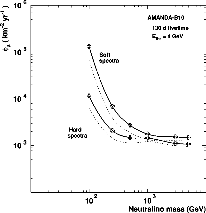
Figures 9 and 10 show the 90% confidence level limit on the

FIG. 9. 90% confidence level upper limits on the neutralino

annihilation rate,

, in the center of the Earth as a function of the

neutralino mass and for the two extreme annihilation channels con

sidered in the analysis. The dashed lines indicate the limits obtained

without including systematic uncertainties and correspond to the

numbers in parentheses in Table III. The symbols indicate the

masses used in the analysis. Lines are to guide the eye.

FIG. 10. 90% confidence level upper limits on the muon flux at

the surface of the Earth,

, as a function of the neutralino mass

and for the two extreme annihilation channels considered in the

analysis. The dashed lines indicate the limits obtained without in

cluding systematic uncertainties and correspond to the numbers in

parentheses in Table III. The symbols indicate the masses used in

the analysis. Lines are to guide the eye.

J. AHRENS

et al.

PHYSICAL REVIEW D

, 032006

2002

03200610

neutralino annihilation rate and the corresponding limit on

the resulting muon flux for a muon threshold of 1 GeV for

the hard and soft annihilation channels considered in the

analysis. The symbols show the particular neutralino masses

used in the simulation. The lines are to guide the eye and

they show the limits obtained, including systematic uncer

tainties

solid line

. The dashed lines, included for compari

son, show the values obtained using the Neyman construc

tion with the unified ordering scheme without including

uncertainties. Table III summarizes the corresponding num

bers.

C. Effect of neutrino oscillations

To account for neutrino oscillations among the different

flavors, the atmospheric neutrino spectrum should be

weighted by a factor

(

), which includes the probability

that a muon neutrino has oscillated into another flavor in its

way through the Earth to the detector. For the purpose of

illustration consider a twoflavor oscillation scenario

between

and

. Then

(

)

sin

) sin

1.27

(eV

)

(km)/

(GeV)

, where

is the diameter of the Earth,

the mixing angle and

the difference of the squares of the flavor masses. Note that

the effect depends strongly on the neutrino energy and it is

negligible in the high energy tail of the atmospheric spec

trum since the oscillation length is then much larger than the

Earth’s diameter. If we choose sin

)

1 and

2.5

based on the results obtained in Ref.

the number of expected atmospheric neutrino events is re

duced between 5% and 10%, depending on the angular cone

considered. This would weaken the limits by about the same

amount.

The effect of neutrino oscillations on the possible WIMP

signal is model dependent and has been estimated in Refs.

and

. However the authors reach different conclu

sions on the direction of the effect: up to a factor of two in

increased muon flux in Ref.

and a reduction of about

25% in Ref.

for a neutralino mass of 100 GeV. For

higher neutralino masses both authors predict a less pro

nounced effect, which becomes negligible for the higher

masses considered in

(

300 GeV). We have not

included any oscillation effect on the neutrinos from the

WIMP signals considered in this paper.

VIII. COMPARISON WITH OTHER EXPERIMENTS AND

THEORETICAL MODELS

Searches for a neutrino signal from WIMP annihilation in

the center of the Earth have been performed by MACRO,

Baikal, Baksan, and SuperKamiokande.

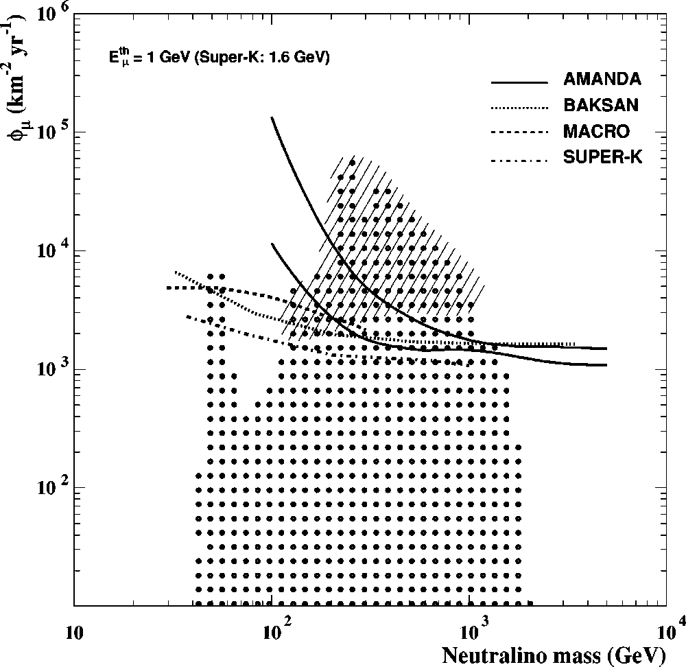
In Fig. 11 the results of Baksan

, MACRO

and

SuperKamiokande

are shown along with the limits

from AMANDA obtained in the previous section and

theoretical predictions of the MSSM as a function of WIMP

mass. In order to be able to compare with the other experi

ments, the SuperKamiokande limits have been scaled by a

factor 1/0.9 to represent total flux limits, instead of limits

based on angular cones, including 90% of the signal as origi

nally presented in Ref.

. The 90% confidence level muon

flux limits for a muon energy threshold of 10 GeV published

by the Baikal collaboration range between

0.63

for a zenith half cone of 15° and

0.54

for a zenith half cone of 5°

Ref.

. Since these results are not presented as a function of

WIMP mass, and are quoted at a slightly higher muon energy

threshold, we have not included them in the figure but we

mention them here for completeness.

Each point in the figure represents a flux obtained with a

particular combination of MSSM parameters, following Ref.

. The original 64 free parameters of the general MSSM

have been reduced to seven by the standard assumptions

about the behavior of the theory at the grand unified scale

and about the supersymmetry breaking parameters in the

fermion sector. The independent parameters left are the

Higgsino mass parameter

, the ratio of the Higgs vacuum

expectation values tan

, the gaugino mass parameter

the mass

of the

odd Higgs boson and the quantities

and

from the ansatz on the scale of supersymme

try breaking. These parameters were varied in the following

ranges:

5000

5000 GeV,

5000

5000 GeV, 1.2

tan

50,

1000 GeV, 100

3000 GeV,

and

Models based on parameters already excluded by accelerator

limits are not shown, and the figure is restricted to those

models which give cosmologically interesting neutralino

relic densities, 0.025

0.5. A local dark matter den

sity of 0.3 GeV/cm

has been assumed. Theoretical predic

tions for high mass neutralino models lie below the scale of

FIG. 11. The AMANDA limits on the muon flux from neutralino

annihilations from Fig. 10 compared with published limits from

MACRO, Baksan and SuperKamiokande. The dots represent

model predictions from the MSSM, calculated with the DarkSUSY

package

. The dashed area shows the models disfavored by

direct searches from the DAMA collaboration as calculated in

LIMITS TO THE MUON FLUX FROM WIMP... PHYSICAL REVIEW D

, 032006

2002

03200611

the plot, since in this case the number density of neutralinos

falls down rapidly if the dark matter density is kept fixed.

A complementary way to search for neutralinos is by

measuring the nuclear recoil in elastic neutralinonucleus

collisions on an adequate target material

. Experiments

using this direct detection technique set limits on the

neutralinonucleon cross section as a function of neutralino

mass. The same scan over MSSM parameter space used to

generate the theoretical points in Fig. 11 can be used to iden

tify parameter combinations that are accessible by direct

searches. There is not, however, a onetoone correspondence

between the results of the direct detection searches and the

expected neutrino flux from the models probed, so compari

sons with the results of indirect searches have to be per

formed with care. We have indicated the models disfavored

by the DAMA Collaboration

by the dashed area in the

figure, which has to be taken as an approximate region in

view of the mentioned difficulties in comparing both types of

detection techniques. We note that the models that yield high

muon fluxes, and that are disfavored by both current results

from direct searches and by the limits shown in the figure,

have in common a low value of the H

mass, around 92 GeV.

IX. SUMMARY

We have performed a search for a statistically significant

excess of vertically upgoing muons with the AMANDA

neutrino detector as a signature for neutralino annihilation in

the center of the Earth. Limits on the neutralino annihilation

rate have been derived from the nonobservation of a signal

excess over the predicted atmospheric neutrino background.

We have included the effect of the detector systematic uncer

tainties and the theoretical uncertainty in the expected num

ber of background events in the derivation of the limits, pre

senting in this way realistic limit values.

A comparison with the results of MACRO, SuperK and

Baksan, as well as with theoretical expectations from the

MSSM, is presented. AMANDA, with only 130.1 days of

effective exposure in 1997, has reached a sensitivity in the

high neutralino mass (

500 GeV) region comparable to

that achieved by detectors with much longer livetimes.

ACKNOWLEDGMENTS

AMANDA is supported by the following agencies: The

U.S. National Science Foundation, the University of Wiscon

sin Alumni Research Foundation, the U.S. Department of

Energy, the U.S. National Energy Research Scientific Com

puting Center, the Swedish Research Council, the Swedish

Polar Research Council, the Knut and Allice Wallenberg

Foundation

Sweden

and the German Federal Ministry of

Education and Research. D. F. Cowen acknowledges the sup

port of the NSF CAREER program. C. P. de los Heros ac

knowledges support from the EU 4th framework of Training

and Mobility of Researches. P. Loaiza was supported by the

Swedish STINT program. We acknowledge the invaluable

support of the AmundsenScott South Pole station personnel.

We are thankful to I. F. M. Albuquerque and W. Chinowsky

for their careful reading of the manuscript and valuable com

ments.

L. Bergstro

m, Rep. Prog. Phys.

, 793

2000

G. Jungman, M. Kamionkowski, and K. Griest Phys. Rep.

267

195

1996

K. Griest and M. Kamionkowski, Phys. Rev. Lett.

, 615

1990

G. Abbiendi

et al.

, Eur. Phys. J. C

2000

;

, 187

2000

J. Edsjo

and P. Gondolo, Phys. Rev. D

, 1879

1997

W.H. Press and D.N. Spergel, Astrophys. J.

296

, 679

1985

K. Freese, Phys. Lett.

167B

, 295

1986

; T. Gaisser, G. Steig

man, and S. Tilav, Phys. Rev. D

, 2206

1986

A. Gould, Astrophys. J.

328

, 919

1988

J.L. Feng, K.T. Matchev, and F. Wilczek, Phys. Rev. D

045024

2001

E. Andre

et al.

, Astropart. Phys.

2000

E. Andre

et al.

, Nature

London

410

,411

2001

; J. Ahrens

et al.

, Phys. Rev. D

, 012005

2002

R. Wischnewski,

et al.

, Proceedings of the XVII International

Cosmic Ray Conference

ICRC

, Hamburg, Germany, p. 1105;

S. Barwick,

et al.

ibid

., p. 1101.

J. Edsjo

, Ph.D. thesis. Uppsala University, 1997,

hepph/9704384; L. Bergstro

m, J. Edsjo

, and P. Gondolo,

Phys. Rev. D

, 103519

1998

T. Sjo

strand Comput. Phys. Commun.

,74

1994

P. Lipari, Astropart. Phys.

, 195

1993

R. Ghandi

et al.

, Astropart. Phys.

,81

1996

H.L. Lai

et al.

, Phys. Rev. D

, 4763

1995

E. Dalberg, Ph.D. thesis, Stockholm University, 1999, ISBN

9172650249.

S.N. Boziev

et al.

, INR preprint P0630, Moscow, 1989.

T.K. Gaisser,

Cosmic Rays and Particle Physics

Cambridge

University Press, Cambridge, England, 1990

D. Heck

et al.

, FZKA report 6019, 1998, http://ik1au1.fzk.de/

heck/corsika/

Particle Data Group, D. Groom

et al.

, Eur. Phys. J. C

2000

W. Lohmann

et al.

, CERN Yellow Report CERNEP/8503,

1985.

G. Hill

et al.

, in Proceedings of the XVI International Cosmic

Ray Conference

ICRC

, Salt Lake City, Utah, 1999,

HE.6.3.02.

V.J. Stenger, University of Hawaii preprint, HDC190

1990

C. Wiebusch, in Proceedings of the International Workshop on

Simulations and Analysis Methods for Large Neutrino Tele

scopes, Zeuthen, Germany, 1998, edited by C. Spiering

DESYPROC199901, 1999

, p. 302.

P. Loaiza, Licentiat thesis, Uppsala University, 2000.

T.G.M. Malmgren, Comput. Phys. Commun.

106

, 230

1997

K. Woschnagg, in Proceedings of the XVI International Cos

mic Ray Conference

ICRC

, Salt Lake City, Utah, 1999,

HE.4.1.15.

J. AHRENS

et al.

PHYSICAL REVIEW D

, 032006

2002

03200612

T. Gaisser,

et al.

, in Proceedings of the XVII International

Cosmic Ray Conference

ICRC

, Hamburg, Germany, 2001, p.

1643.

I. Sokalski

et al.

, Phys. Rev. D

, 074015

2001

D. Chirkin and W. Rhode, in Proceedings of the XVII Interna

tional Cosmic Ray Conference

ICRC

, Hamburg, Germany,

2001, p. 1017.

A. Stuart and J. K. Ord,

Kendall’s Advanced Theory of Statis

tics

Oxford University Press, New York, 1991

, Vol. 2; G.J.

Feldman and R.D. Cousins, Phys. Rev. D

, 3873

1998

R.D. Cousins and V.L. Highland, Nucl. Phys.

A320

, 331

1992

J. Conrad

et al.

, in Proceedings of the Workshop on Advanced

Statistical Techniques in Particle Physics, Durham, UK, 2002,

hepex/0202013.

J. Kameda

et al.

, in Proceedings of the XVII International

Cosmic Ray Conference

ICRC

, Hamburg, Germany, 2001, p.

1057.

M. Kowalski, Phys. Lett. B

511

,119

2001

N. Fornengo, in Proceedings of the Third International Confer

ence on Dark Matter in Astro and Particle Physics, Heidelberg,

Germany, 2000. Also hepph/0011030.

P. Gondolo,

et al.

Proceedings of the Third International

Workshop on Identification of Dark Matter (IDM2000),

York,

UK, 2000, edited by N.J.C. Spooner and V. Kudryavtsev

World Scientific, Singapore, 2001

, p. 318; P. Gondolo,

astroph/0012234; http://www.physto.se/

edsjo/darksusy/.

M. Boliev

et al.

,in

Proceedings of Dark Matter in Astro and

Particle Physics, 1997

, edited by H.V. KlapdorKleingrothaus

and Y. Ramachers

World Scientific, Singapore, 1997

,p.711;