.
Astroparticle Physics 13 2000 1–20
www.elsevier.nl
r
locate
r
astropart
The AMANDA neutrino telescope: principle of operation and
first results
E. Andres
j
, P. Askebjer
d
, S.W. Barwick
f,
)
, R. Bay
e
, L. Bergstrom
d
, A. Biron
b
,
¨
J. Booth
f
, A. Bouchta
b
, S. Carius
c
, M. Carlson
h
, D. Cowen
g
, E. Dalberg
d
,
T. DeYoung
h
, P. Ekstrom
d
, B. Erlandson
d
, A. Goobar
d
, L. Gray
h
, A. Hallgren
k
,
¨
F. Halzen
h
, R. Hardtke
h
, S. Hart
j
,Y.He
e
, H. Heukenkamp
b
, G. Hill
h
,
P.O. Hulth
d
, S. Hundertmark
b
, J. Jacobsen
i
, A. Jones
j
, V. Kandhadai
h
, A. Karle
h
,
B. Koci
h
, P. Lindahl
c
, I. Liubarsky
h
, M. Leuthold
b
, D.M. Lowder
e
,
P. Marciniewski
k
, T. Mikolajski
b
, T. Miller
a
, P. Miocinovic
e
, P. Mock
f
,
R. Morse
h
, P. Niessen
b
, C. Perez de los Heros
k
, R. Porrata
f
, D. Potter
j
,
´
P.B. Price
e
, G. Przybylski
i
, A. Richards
e
, S. Richter
j
, P. Romenesko
h
,
H. Rubinstein
d
, E. Schneider
f
, T. Schmidt
b
, R. Schwarz
j
, M. Solarz
e
,
G.M. Spiczak
a
, C. Spiering
b
, O. Streicher
b
, Q Sun
d
, L. Thollander
d
,
T. Thon
b
, S. Tilav
h
, C. Walck
d
, C. Wiebusch
b
, R. Wischnewski
b
,
K. Woschnagg
e
, G. Yodh
f
a
Bartol Research Institute, Uni
˝
ersity of Delaware, Newark, DE, USA
b
DESYZeuthen, Zeuthen, Germany
c
Kalmar Uni
˝
ersity, Sweden
d
Stockholm Uni
˝
ersity, Stockholm, Sweden
e
Uni
˝
ersity of California Berkeley, Berkeley, CA, USA
f
Uni
˝
ersity of California Ir
˝
ine, Ir
˝
ine, CA, USA
g
Uni
˝
ersity of Pennsyl
˝
ania, Philadelphia, PA, USA
h
Uni
˝
ersity of Wisconsin, Madison, WI, USA
i
Lawrence Berkeley Laboratory, Berkeley, CA, USA
j
South Pole Station, Antarctica
k
Uni
˝
ersity of Uppsala, Uppsala, Sweden
Received 25 May 1999; accepted 21 June 1999
Abstract
AMANDA is a highenergy neutrino telescope presently under construction at the geographical South Pole. In the
. .
Antarctic summer 1995
r
96, an array of 80 optical modules OMs arranged on 4 strings AMANDAB4 was deployed at
)
Corresponding author.
.
Email address:
sbarwick@uci.edu S.W. Barwick .
09276505
r
00
r
$ see front matter
q
2000 Elsevier Science B.V. All rights reserved.
.
PII: S0927 6505 99 000924
()
E. Andres et al.
r
Astroparticle Physics 13 2000 1–20
2
depths between 1.5 and 2 km. In this paper we describe the design and performance of the AMANDAB4 prototype, based
on data collected between February and November 1996. Monte Carlo simulations of the detector response to downgoing
atmospheric muon tracks show that the global behavior of the detector is understood. We describe the data analysis method
and present first results on atmospheric muon reconstruction and separation of neutrino candidates. The AMANDA array
.
was upgraded with 216 OMs on 6 new strings in 1996
r
97 AMANDAB10 , and 122 additional OMs on 3 strings in
1997
r
98.
q
2000 Elsevier Science B.V. All rights reserved.
1. Introduction
Techniques are being developed by several groups
to use high energy neutrinos as a probe for the
highest energy phenomena observed in the Universe.
Neutrinos yield information complementary to that
obtained from observations of high energy photons
and charged particles since they interact only weakly
and can reach the observer unobscured by intervent
ing matter and undeflected by magnetic fields.
The primary mission of large neutrino telescopes
is to probe the Universe in a new observational
window and to search for the sources of the highest
energy phenomena. Presently suggested candidates
for these sources are, for instance, Active Galactic
. .
Nuclei AGN and Gamma Ray Bursts GRB . A
neutrino signal from a certain object would consti
tute the clearest signature of the hadronic nature of
wx
that cosmic accelerator 1 . Apart from that, neutrino
telescopes search for neutrinos produced in annihila
tions of Weakly Interacting Massive Particles
.
WIMPs which may have accumulated in the center
of the Earth or in the Sun. WIMPS might contribute
to the cold dark matter content of the Universe, their
detection being of extreme importance for cosmol
wx
ogy 2,3 . Neutrino telescopes can be also used to
wx
monitor the Galaxy for supernova explosions 4 and
to search for exotic particles like magnetic monopoles
wx
5,6 . In coincidence with surface air shower arrays,
deep neutrino detectors can be used to study the
chemical composition of charged cosmic rays. Fi
nally, environmental investigations – oceanology or
limnology in water, glaciology in ice – have proved
wx
to be exciting applications of these devices 7,9 .
Planned highenergy neutrino telescopes differ in
many aspects from existing underground neutrino
detectors. Their architecture is optimized to achieve
a large detection area rather than a low energy
threshold. They are deployed in transparent ‘‘open’’
media like water in oceans or lakes, or deep polar
ice. This brings additional inherent technological
challenges compared with the assembly of a detector
in an accelerator tunnel or underground cavities.
Neutrinos are inferred from the arrival times of
Cherenkov light emitted by charged secondaries pro
duced in neutrino interactions. The light is mapped
.
by photomultiplier tubes PMTs spanning a coarse
threedimensional grid.
The traditional approach to muon neutrino detec
tion is the observation of upward moving muons
produced in charged current interactions in the rock,
water or ice below the detector. The Earth is used as
a filter with respect to atmospheric muons. Still,
suppression of downwardgoing muons is of top
importance, since their flux exceeds that of upward
going muons from atmospheric neutrinos by several
orders of magnitude.
An array of PMTs can also be used to reconstruct
the energy and location of isolated cascades due to
neutrino interactions. Burstlike events, like the onset
of a supernova, might be detected by measuring the
increased count rates of all individual PMTs.
Technologies for under
water
telescopes have been
pioneered by the since decommissioned DUMAND
wx
project near Hawaii 11,12 and by the Baikal collab
wx
oration 7,10 . In contrast to these approaches, the
wx
AMANDA detector 15 used deep polar ice as target
and radiator. Two projects in the Mediterranean,
wx wx
NESTOR 13 and ANTARES 14 , have joined the
worldwide effort towards largescale underwater
telescopes. BAIKAL and AMANDA are presently
taking data with first stage detectors.
The present paper describes results obtained with
.
the first four out of the current thirteen strings of
the AMANDA detector. The paper is organized as
follows: In Section 2 we give a general overview of
()
E. Andres et al.
r
Astroparticle Physics 13 2000 1–20
3
the AMANDA concept. Section 3 summarizes the
results obtained with a shallow survey detector called
AMANDAA. Section 4 describes the design of the
first four strings of the deeper array AMANDAB4.
Calibration of time response and of geometry are
explained in Section 5. In Section 6 we describe the
simulation and reconstruction methods with respect
to atmospheric muons and compare experimental
data to Monte Carlo calculations. Section 7 demon
strates the performance of AMANDAB4 operated in
coincidence with SPASE, a surface air shower array.
In Section 8, the angular spectrum of atmospheric
muons is derived and transformed into a dependence
of the vertical intensity on depth. Section 9 describes
the separation of first upward going muon candi
dates. Finally, a summary of the status of AMANDA
and results is presented in Section 10.
2. The AMANDA concept
AMANDA Antarctic Muon And Neutrino Detec
.
tor Array uses the natural Antarctic ice as both
target and Cherenkov medium. The detector consists
.
of strings of optical modules OMs frozen in the 3
km thick ice sheet at the South Pole. An OM consists
of a photomultiplier in a glass vessel. The strings are
deployed into holes drilled with pressurized hot wa
ter. The water column in the hole then refreezes
within 35–40 hours, fixing the string in its final
position. In our basic design, each OM has its own
.
cable supplying the high voltage HV as well as
transmitting the anode signal. The components under
the ice are kept as simple as possible, all the data
acquisition electronics being housed in a building at
the surface. The simplicity of the components under
ice and the nonhierarchical structure make the de
tector highly reliable.
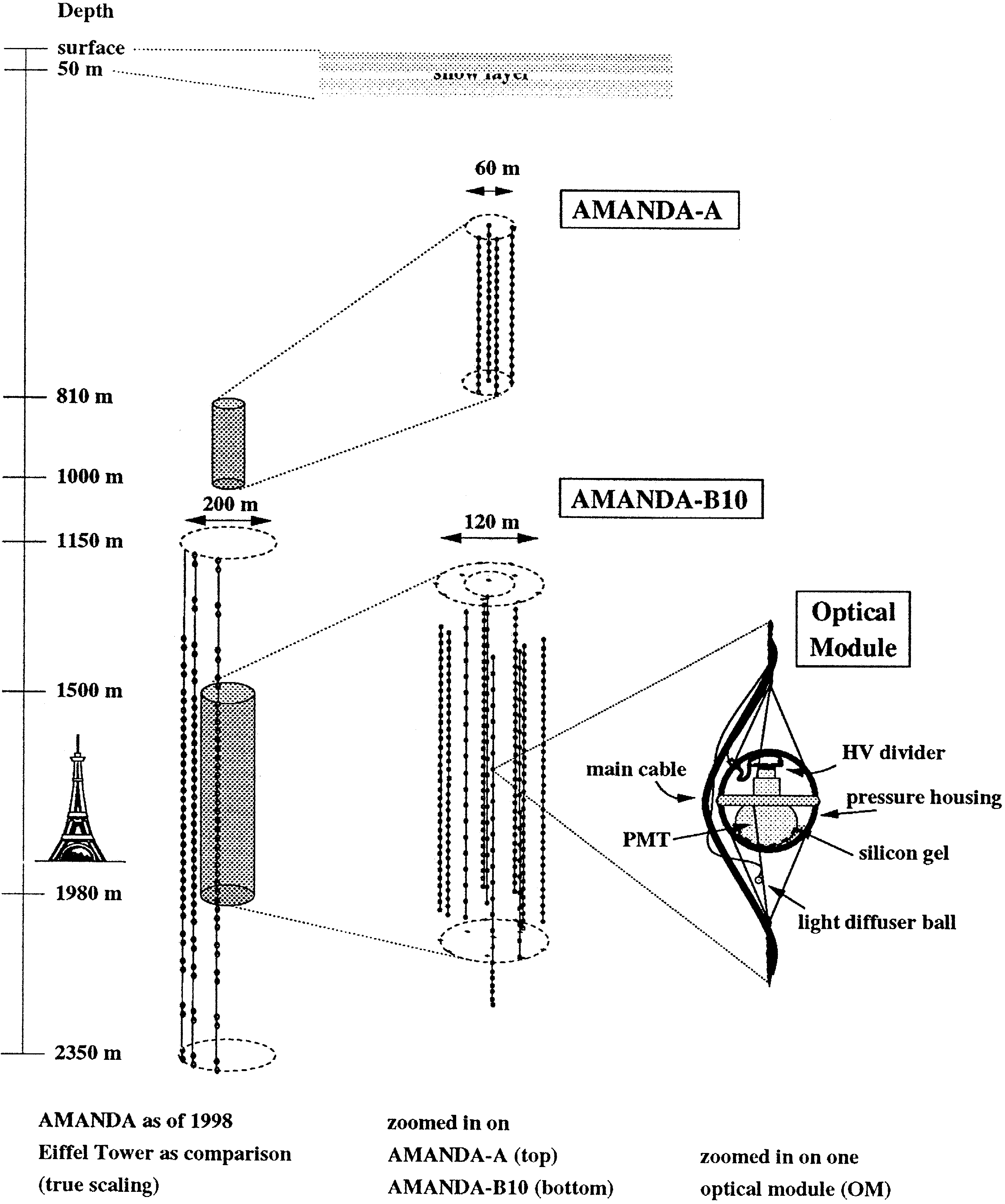
Fig. 1 shows the current configuration of the
AMANDA detector. The shallow array, AMANDA
A, was deployed at a depth of 800 to 1000 m in
1993
r
94 in an exploratory phase of the project.
Studies of the optical properties of the ice carried out
with AMANDAA showed that a high concentration
of residual air bubbles remaining at these depths
leads to strong scattering of light, making accurate
wx
track reconstruction impossible 8 . Therefore, in the
polar season 1995
r
96 a deeper array consisting of
.
80 OMs arranged on four strings AMANDAB4
was deployed at depths ranging from 1545 to 1978
meters, where the concentration of bubbles was pre
dicted to be negligible according to extrapolation of
AMANDAA results. The detector was upgraded in
1996
r
97 with 216 additional OMs on 6 strings. This
detector of 4
q
6 strings was named AMANDAB10
and is sketched at the right side of Fig. 1.
AMANDAB10 was upgraded in the season 1997
r
98
by 3 strings instrumented between 1150 m and 2350
m which fulfill several tasks. Firstly, they explore
the very deep and very shallow ice with respect to a
future cube kilometer array. Secondly, they form one
corner of AMANDAII which is the next stage of
AMANDA with altogether about 700 OMs. Thirdly,
they have been used to test data transmission via
optical fibers.
There are several advantages that make the South
Pole a unique site for a neutrino telescope:
fl
The geographic location is unique: A detector
located at the South Pole observes the northern
hemisphere, and complements any other of the
planned or existing detectors.
fl
Ice is a sterile medium. The noise is given only
by the PMT dark noise and by
40
K decays in the
glass housings, which are 0.5–1.5 kHz for the
PMTs and spheres we used. Ocean and lake
experiments have to cope with 100 kHz noise
40
rates due to bioluminescence or K decays 25–
30 kHz if normalized to the photocathode area of
XX
.
the 8 PMT used in AMANDA . This fact not
only facilitates counting rate experiments like the
search for low energy neutrinos from supernovae
or GRBs, but also leads to fewer accidental hits in
muon events – an essential advantage for trigger
formation and track reconstruction.
fl
AMANDA can be operated in coincidence with
air shower arrays located at the surface. Apart
from complementing the information from the
surface arrays by measurements of muons pene
trating to AMANDA depths, the air shower infor
mation can be used to calibrate AMANDA.
fl
The South Pole station has an excellent infrastruc
ture. Issues of vital importance to run big experi
()
E. Andres et al.
r
Astroparticle Physics 13 2000 1–20
4
.
Fig. 1. Scheme of the 1998 AMANDA installations. The left picture is drawn with true scaling. A zoomed view on AMANDAA top and
.
AMANDAB10 bottom is shown at the center. The right zoom depicts the optical module.
ments like transportation, power supply, satellite
communication and technical support are solved
and tested during many years of operation. Part of
an existing building can be used to house the
surface electronics.
fl
The drilling and deployment procedures are tested
and well under control. AMANDA benefits from
the drilling expertise of the Polar Ice Coring
.
Office PICO . Currently about five days are
needed to drill a hole and to deploy a string with
PMTs to a depth of 2000 m. Future upgrades of
the drilling equipment are expected to result in a
further speedup.
The optical properties of the ice turned out to be
very different from what had been expected before
the AMANDAA phase. Whereas absorption is much
weaker than in oceans, scattering effects turned out
to be much stronger. Even at depths below 1400
meters, where residual bubbles have collapsed al
most completely into air hydrates, scattering is nearly
an order of magnitude stronger than in water see
.
below . Since scattering of light smears out the
arrival times of Cherenkov flashes, a main question
was whether under these conditions track reconstruc
tion was possible. As shown below, the answer is
yes.
()
E. Andres et al.
r
Astroparticle Physics 13 2000 1–20
5
3. AmandaA: a first survey
Preliminary explorations of the site and the drilling
technology were performed in the Antarctic Summer
wx
1991
r
92 15 . During the 1993
r
94 campaign, four
.
strings each carrying 20 OMs ‘‘AMANDAA’’
were deployed between 800 and 1000 m depth. None
XX
.
of the 73 OMs equipped with 8 EMI PMTs
surviving the refreezing process failed during the
following two years, giving a mean time between
.
failures MTBF
)
40 years for individual OMs in
AMANDAA. The OMs are connected to the surface
electronics by coaxial cables. Along with the coaxial
cables, optical fibers carry light from a Nd:YAG
laser at the surface to nylon light diffusers placed
.
about 30 cm below each PMT see Fig. 1 . Time
calibration is performed by sending nanosecond laser
pulses to individual diffusers and measuring the pho
ton arrival time distributions at the closest PMT.
From the distribution of the arrival times at
distant
PMTs, the optical properties of the medium were
wx
derived 8,9 . The measured timing distributions in
dicated that photons do not propagate along straight
paths but are scattered and considerably delayed due
to residual bubbles in the ice. The distributions could
be fitted well with an analytic function describing
.
the threedimensional random walk scattering in
cluding absorption. These results showed that polar
ice at these depths has a very large absorption length,
exceeding 200 m at a wavelength of 410 nm. Scatter
ing is described by the effective scattering length
:.
L
s
L
r
1
y
cos
u
, where
L
is the geometri
eff sc sc
:
cal scattering length and cos
u
the average cosine
wx
of the scattering angle 8 .
L
increases with depth,
eff
from 40 cm at 830 m depth to 80 cm at 970 m. In
accordance with measurements at the Vostok Station
wx
.
East Antarctica 16 and Byrd Station West
.
Antarctica these results suggested that at depths
greater than 1300–1400 m the phase transformation
from bubbles into airhydrate crystals would be com
plete and bubbles would disappear.
Although not suitable for track reconstruction,
AMANDAA can be used as a calorimeter for en
ergy measurements of neutrinoinduced cascadelike
wx
events 18 . It is also used as a supernova monitor
wx
17 . Events that simultaneously trigger AMANDAA
and the deeper AMANDAB have been used for
methodical studies like the investigation of the opti
cal properties of the ice or the assessment of events
with a lever arm of one kilometer.
4. Deployment and design of AMANDAB4
4.1. Drilling and deployment procedure
Drilling is performed by melting the ice with
pressurized water at 75
8
C. The drilling equipment
operates at a power of 1.9 MW and the typical drill
speed is about 1 cm
r
s. It takes about 3.5 days to
drill a 50–60 cm diameter hole to 2000 m depth.
In the season 1995
r
96, we drilled four holes, the
deepest of them reaching 2180 m. It took typically 8
hours to remove the drill and the water recycling
pump from the completed hole. The deployment of
one string with 20 OMs and several calibration
devices took about 18 hours with a limit of 35 hours
.
set by the refreezing of the water in the hole .
Several diagnostic devices allow monitoring of
the mechanical and thermal parameters during the
entire refreezing process and afterwards. It was
shown that the temperature increases with depth in
good agreement with the prediction of a standard
heat flow calculation for South Pole ice. At the
greatest depth, the temperature of the ice is
f
y
31
8
C, about 20
8
warmer than at the surface. Dur
ing the refreezing, the pressure reached a maximum
of 460 atm, more than twice the hydrostatic pressure
which is asymptotically established.
4.2. Detector design
The four strings of AMANDAB4 were deployed
at depths between 1545 and 1978 m. An OM con
sists of a 30 cm diameter glass sphere equipped with
a8
XX
Hamamatsu R59122 photomultiplier, a 14dy
node version of the standard 12dynode R5912 tube.
The PMTs are operated at a gain of 10
9
in order to
drive the pulses through 2 km of coaxial cable
without insitu amplification. The amplitude of a
onephotoelectron pulse is about 1 V. The coaxial
cable is also used for the HV supply, with the
advantage that only one cable and one electrical
penetrator into the sphere are required for each OM.
The measured noise rate of the AMANDAB4 PMTs
.
is typically 400 Hz threshold 0.4 photoelectrons .
()
E. Andres et al.
r
Astroparticle Physics 13 2000 1–20
6
Fig. 2. AMANDAB4: Top view, with distances between strings
given in meters, and side view showing optical modules and
calibration light sources. Upward looking PMTs are marked by
arrows.
The photocathode is in optical contact with the
glass sphere by the use of silicon gel. The transmis
sion of the glass of the pressure sphere is about 90%
in the spectral range between 400 and 600 nm; the
50% cutoff on the UV side is at about 365 nm. The
glass spheres are designed to withstand pressures of
about 660 atm.
Each string carries 20 OMs with a vertical spac
ing of 20 m. The fourth string carries six additional
OMs connected by a twisted pair cable. These six
OMs will not be used in the analyses presented in
this paper.
Fig. 2 shows a schematic view of AMANDAB4.
All PMTs look down with the exception of
a
1, 10
in strings 1 to 3 and
a
1, 2, 10, 19, 20 in string 4
with the numbers running from top to bottom of a
.
string . Strings 1–3 form a triangle with side lengths
77–67–61 m; string 4 is close to the center. The
.
OMs are arranged at depths 1545–1925 m string 1 ,
. .
1546–1926 m string 2 , 1598–1978 m string 3
.
and 1576–1956 m string 4 . The additional six OMs
equipped with twisted pair cables are at string 4
between 2009 and 2035 m. Seven of the 80 PMTs
which define AMANDAB4 were lost due to over
pressure and shearing forces to the electrical connec
tors during the refreezing period. These losses can be
reduced by computer controlled drilling avoiding
strong irregularities in the hole diameter, and by
improved connectors. Another 3 PMTs failed in the
course of the first 3 years of operation, giving a
MTBF of 73 years.
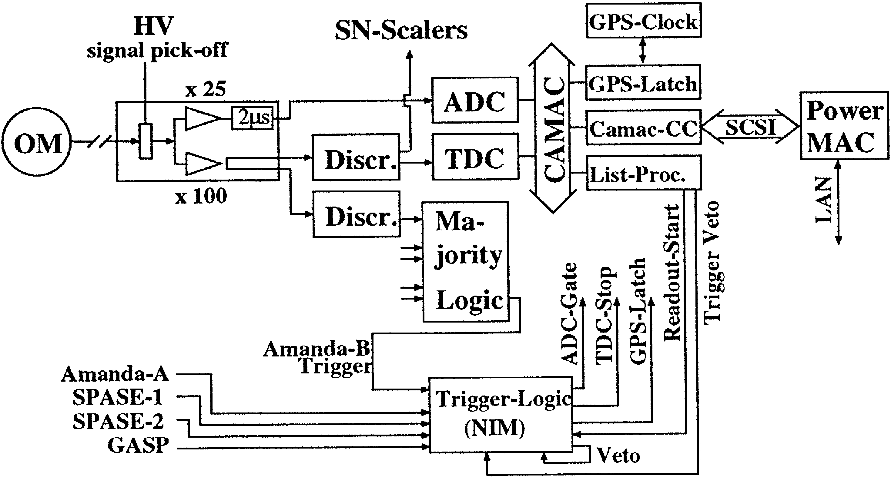
4.3. Electronics and DAQ
Each PMT can give a series of pulses which can
be resolved if separated from each other by more
than a few hundred nanoseconds. The data recorded
consist of the leading and trailing edges of the
pulses. The timeoverthreshold gives a measure of
the amplitude of individual pulses. Another measure
of the amplitude is obtained by a voltage sensitive
ADC which records the peak value out of the subse
quent hits of an event in a PMT. Actually, the
information consists of leading and trailing edges of
the last 8 resolved pulses, and of the largest ampli
tude of those of them which lie in a 4
m
sec window
centered at the array trigger time. Also recorded is
the GPS time at which the event occurred. A scheme
of the AMANDA electronics layout is shown in Fig.
3.
The signal from each cable is fed to a module
consisting of a DC blocking highpass filter which
picks up the pulse, a fanout sending it to 2 ampli
fiers with 100
=
and 25
=
gain, and a 2
m
sec delay
for the lowgain signal.
The delayed signal is sent to a Phillips 7164 peak
sensing ADC. The other pulse is split and sent to
Fig. 3. DAQ system used for AMANDAB4 during 1996
()
E. Andres et al.
r
Astroparticle Physics 13 2000 1–20
7
LeCroy 4413 discriminators with thresholds set at
100 mV corresponding to about 0.3–0.4 photoelec
trons at the given high voltage. One of the resulting
ECL pulses is fed into a LeCroy 3377 TDC while
the other is sent to the majority trigger. The TDC
records the last 16 time edges occurring within a 32
m
sec time window.
The majority logic requests
G
8 hit PMTs within
a sliding window of 2
m
sec. The trigger produced by
this majority scheme is sent to the NIM trigger logic.
The latter accepts also triggers from AMANDAA or
the air shower experiments SPASE1, SPASE2 and
GASP. Thus AMANDA also records data when
these detectors trigger even if a proper AMANDA
trigger is not fulfilled. The total trigger rate during
1996 was about 26 Hz on average. The coincidences
from the other detectors contributed about 8 Hz to
the total rate.
The differences in cable length are not compen
sated before triggering. Therefore the true trigger
window would be about 300 nsec for a vertically
upgoing relativistic particle and
f
4
m
sec for a
downgoing one. As a result downgoing particles are
suppressed compared to upgoing.
Upon triggering, an ADC gate of 4
m
sec width is
formed, a stop signal is sent to the TDCs and a
readout signal is sent to a Hytec LP1341 list proces
sor. Then a veto lasting several microseconds in
hibits further trigger signals.
.
A separate system ‘‘SN scalers’’ in Fig. 3 moni
tors the counting rates of individual PMTs and
searches for rate excesses lasting several seconds.
Such an increase would be expected for multiple
lowenergy neutrino interactions close to each PMT
wx
due to a supernova burst 4,17 .
The AMANDAB4 DAQ was running on a Mac
Intosh Power PC communicating through a SCSI bus
with the CAMAC crate controller. From the distribu
tion of the time differences between subsequent
events, the dead time of the DAQ is estimated to be
about 12%. The MacIntosh has been replaced by a
PentiumII PC running under LINUX in 1998, and
part of the CAMAC electronics by VME modules.
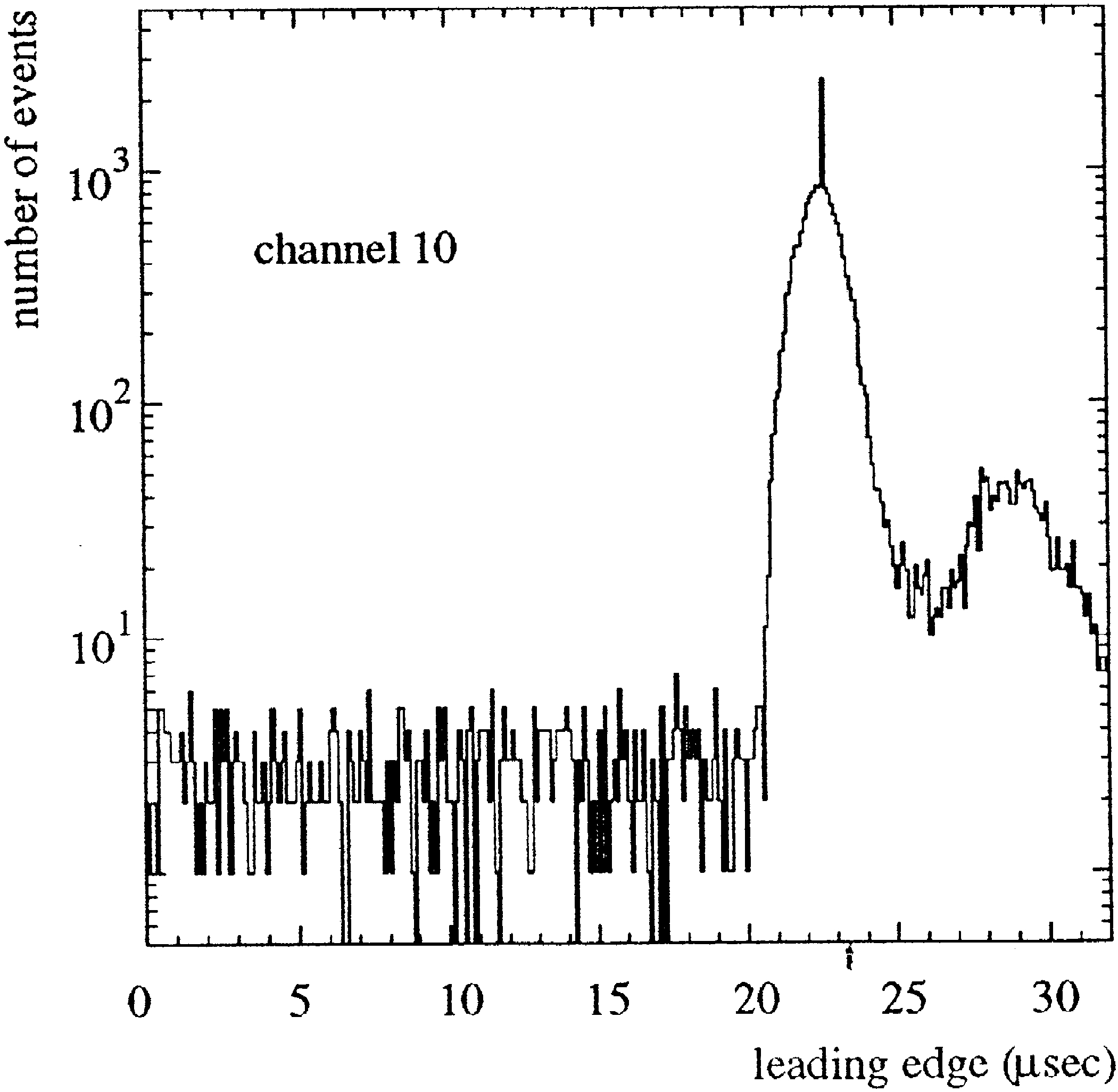
Fig. 4 shows the distribution of the leadingedge
times of one PMT for data taken with the 8fold
majority trigger. The sharp peak at 23
m
sec is given
by the time when this PMT was the triggering one
.
i.e. the eighth within a 2
m
sec window. The flat
Fig. 4. Leading edge times of PMT
a
10 of AMANDAB4 for
data taken with an 8fold majority trigger.
part is due to noise hits and the bulge after the main
.
distribution to afterpulses about 6% .
4.4. Calibration light sources and ice properties
An essential ingredient to the operation of a detec
tor like AMANDA is the knowledge of the optical
properties of the ice, as well as a precise time
calibration of the detector. Various light calibration
sources have been deployed at different depths in
order to tackle these questions:
fl
The YAG laser calibration system
. It uses optical
fibers with diffusers located at each PMT. This
system is similar to that used for AMANDAA.
The range of transmittable wavelength is
G
450
nm, the time resolution is about 15 nsec at 530
nm, the maximum intensity emitted by the dif
fusers is 10
8
photons
r
pulse. Apart from ice in
vestigations, the laser system is used for time
calibration of the PMT closest to the diffuser and
.
for position calibration see Section 5 .
fl
A nitrogen laser
at 1850 m depth, wavelength
337 nm, pulse duration 1 nsec, with a maximum
intensity of 10
10
photons
r
pulse.
fl
Three DC halogen lamps
one broadband and two
.
with filters for 350 and 380 nm , maximum inten
14
.
18
.
sity 10 UVfiltered and 10 broadband pho
tons
r
second.
fl
LED beacons
, operated in pulsed mode 500 Hz,
6
.
pulse duration 7 nsec, 10 photons
r
pulse and
14 15
.
DC mode 10 to 10 photons
r
sec , wave
length 450 nm. A filter restricts the output of a
few beacons at 390 nm, with reduced intensity.
()
E. Andres et al.
r
Astroparticle Physics 13 2000 1–20
8
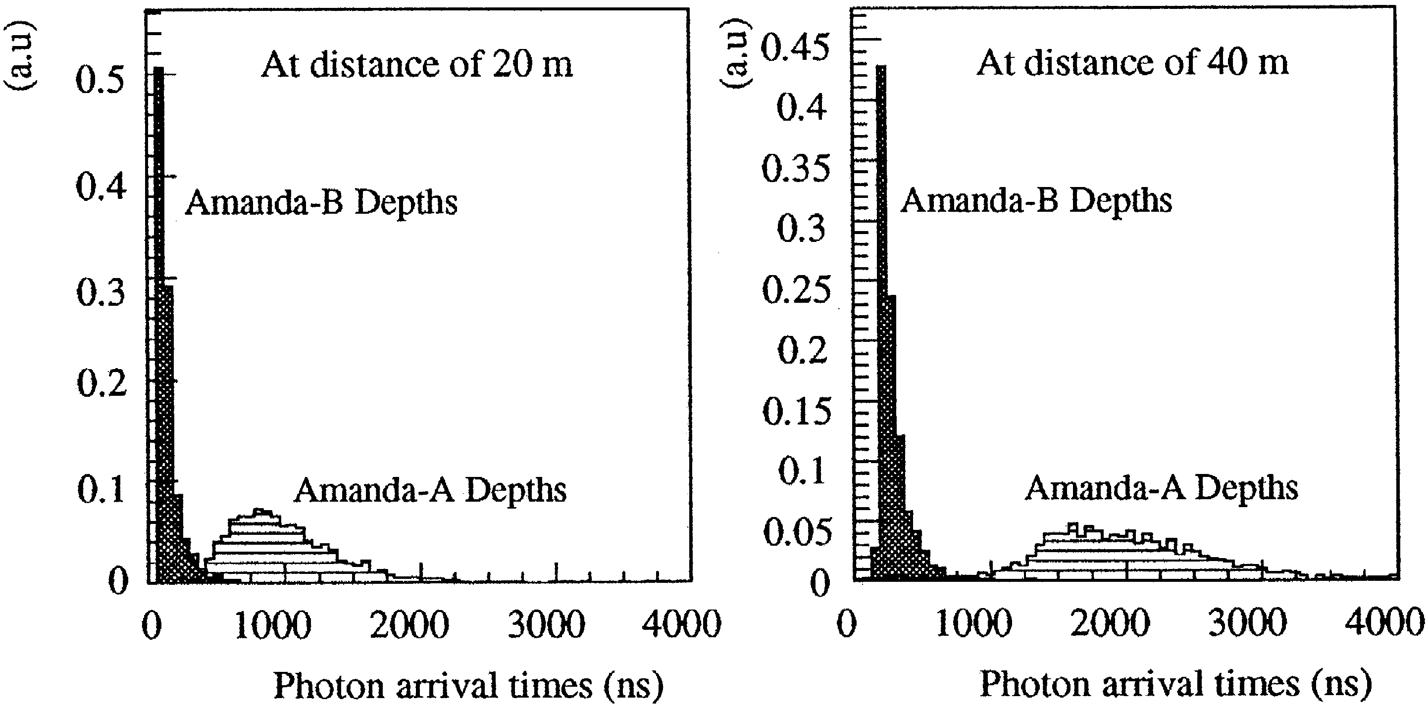
Fig. 5. Arrival time distributions for 510 nm photons for two
sourcedetector distances. Black histograms: AMANDAB.
Hatched histograms: AMANDAA. The histograms are normal
ized to the same area.
Timeofflight measurements have been made for
a large variety of combinations of optical fiber emit
ters and PMTs for the YAG laser system, and at
different wavelengths and intensities. The nitrogen
laser provided data at 337 nm. The result is a
considerable database of hundreds of time distribu
tions. The width of the distributions is sensitive
predominantly to scattering and the tail to absorption
wx
.
see 30 for details . The DC sources provide data
for attenuation, i.e. the combined effect of absorption
and scattering.
The YAG laser results indicate a dramatic im
provement compared to AMANDAA results. Fig. 5
shows the distributions of arrival time for sourcede
tector distances of 20 and 40 m, respectively, for
AMANDAA as well as AMANDAB depths. The
much smaller widths for AMANDAB support the
expectation that bubbles as the dominant source of
scattering have mostly disappeared at depths be
wx
tween 1550 and 1900 m 16 .
Details of the analysis of the optical properties of
the ice at AMANDAB4 depths have been published
wx
elsewhere 19 . Final results will be published in a
separate paper. The preliminary results can be sum
marized as follows: The absorption length
l
is
ab s
about 95 m for wavelengths between 337 and 480
nm and decreases to 45–50 m at 510 nm. The
effective scattering length
l
is about 24 m. The
eff
attenuation length
l
which characterizes the de
att
crease of the photon flux as a function of the dis
tance is about 27 m. These values are averages over
the full depth interval covered by AMANDAB4.
The variation of attenuation over this depth range is
within
"
30%.
5. Calibration of time response and geometry
5.1. Time calibration
The measured arrival times from each PMT have
to be corrected for the time offset
t
, that is, the time
0
it takes a signal to propagate through the PMT and
the coaxial cable and get digitized by the DAQ. The
time offset is determined by sending light pulses
from the YAG laser to the diffuser nylon balls
located below each OM. Two fibers are available for
each PMT, one single and one multimodal. The
time it takes for light to travel though the fiber is
measured using an OTDR Optical Time Domain
.
Reflectometer and subtracted from the time distribu
tions recorded.
For each PMT, the time difference between the
laser pulse at the surface and the PMT response
arriving back is measured. Upon arrival at the sur
face, the pulses have traveled through nearly 2000
meters of cable and are dispersed, with typical time
overthresholds of 550 nsec and rise times of 180
nsec. The threshold used for TDC measurements is
set to a constant value with the consequence that
small pulses will reach that value later than larger
ones. This causes an amplitudedependent offset or
‘‘time walk’’, which can be corrected for by
’
t
s
t
y
t
y
a
r
ADC . 1
.
true LE 0
Here,
t
is the measured leading edge time and
LE
t
the true time at which the light pulse reaches the
true
photocathode. The estimates of the time offset
t
and
0
the timewalk term
a
are extracted from scatterplots
like the one shown in Fig. 6.
The time resolution achieved in this way can be
estimated by the standard deviation of a Gaussian fit
.
Fig. 6. Example of a fitted leading edge with 100
ADC
1200
for module 19 on string 3. The ADC value measures the peak
value of the amplitude.
()
E. Andres et al.
r
Astroparticle Physics 13 2000 1–20
9
to the distribution of time residuals after correction,
yielding 4–7 nsec see Fig. 7 for an OM with 4 nsec
.
resolution . Part of the variation is due to quality
variations of the 1996 optical fibers. Laboratory
measurements yield a Gaussian width of 3.5 nsec
after 2 km cable.
5.2. Position calibration
Information about the exact geometry of the array
can be obtained by different methods. Firstly, the
measured propagation times of photons between dif
ferent light emitters and receivers can be used to
determine their relative positions. Secondly, absolute
positions can be obtained from drill recordings and
pressure sensors.
5.2.1. Laser calibration
The YAG laser, the nitrogen laser and the pulsed
LEDs can be used to infer the OM positions from the
timeofflight of photons between these light sources
and the OMs. The zero time is determined from the
response of the OM closest to the light source which
is triggered by unscattered photons. This PMT is
lowered in voltage in order not to be driven in
saturation, and a time correction accounting for the
longer PMT transit time is added. In contrast to the
close OM, the distant OMs see mostly scattered
photons. However, for a few of the events out of a
series of about 1500 laser pulses, the leading edge
should be produced by photons which are only
slightly scattered. Therefore, the distance between
emitter and OM can be estimated from the earliest
.
events in the timedifference distribution see Fig. 8 .
In order to reduce the sensitivity to fluctuations in
the number of early hits and binning effects, the
whole left flank of the distribution is fitted with a
Fig. 7. Residuals after subtracting the time correction obtained
with the fitted parameters
t
and
a
for module 19 on string 3.
0
The standard deviation of the Gaussian fit is 4 nsec.
Fig. 8. Simulated timeshift distribution for 1500 onephoto
electron events, for a distance of 60 m between emitter and
receiver. A Gaussian smearing of 10 nsec was applied to individ
ual entries. Clear ice would yield a 10 nsec wide peak at 0 nsec.
Gaussian between the maximum of the distribution
.
height0 in Fig. 8 and the first bin with a height
larger than
height1=1/1
–
height
–
. The cor
.
rected ‘‘first’’ time is given by that bin
bin1
for
which the fitted Gaussian yields a height exceeding
height1
. This time has to be corrected further for
the shifts due to scattering which are expected even
for the first bin of the distribution. The corrections
.
were obtained from Monte Carlo MC calculations
and are almost insensitive to variations in absorption
and scattering length of a few meters.
Given the limited number of measured emitterOM
combinations available for AMANDAB4, it would
have been impossible to keep the coordinates of each
OM as free parameters in a global position fit.
Therefore, all strings were assumed to be straight
and parallel and the OMs to be at a fixed vertical
.
distance 20 m relative to each other. For each
emitter covering enough OMs, a graph of the dis
.
tance
dz
between source and OM
i
versus depth
i
.
z
can be drawn see Fig. 9 . The interstring dis
i
Fig. 9. Principle of position measurement.
()
E. Andres et al.
r
Astroparticle Physics 13 2000 1–20
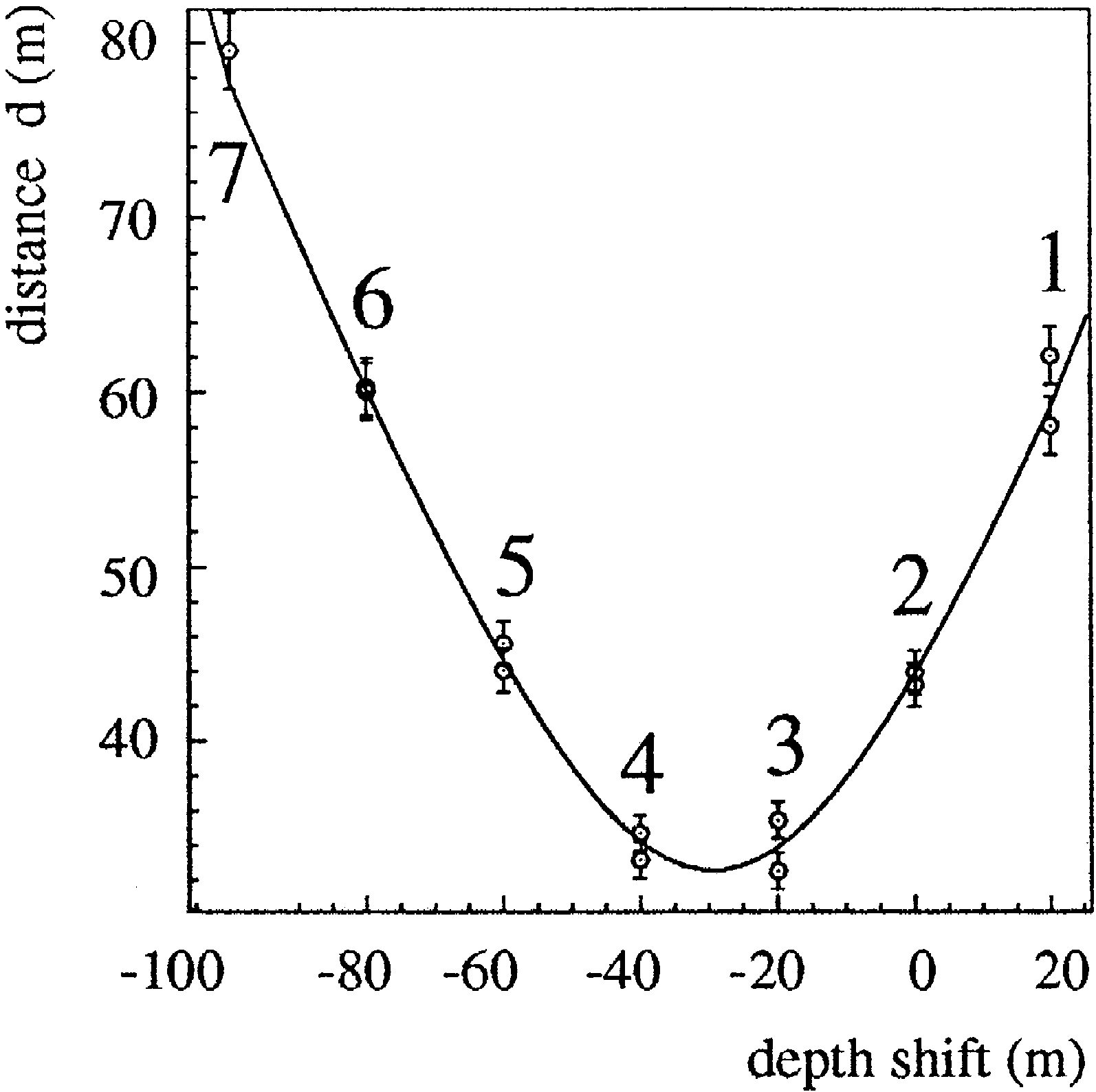
10
.
Fig. 10. Fit of the distance
dz
versus depthshift
z
y
z
be
ii
2
tween OMs at string 4 and a laser emitter at string 2. String
distance
D
and depth shift
z
y
z
are given by the minimum of
02
the parabola.
tance
D
and emitter depth
z
with respect to the
z
0
i
.
can be estimated from this graph by fitting Fig. 10
2
2
(
dz
s
D
q
z
y
z
.2
. . .
ii
0
The residuals from all fits to the 1996 AMANDA
B4 data have a standard deviation of 2 m.
In 1996–1997, six more strings were added on the
outside of the B4 detector, and a new position cali
bration performed. The increased statistics and possi
bilities of new crosschecks and constraints enabled
correction of the existing geometry with an uncer
tainty of 1 m in the horizontal plane and 0.5–1.0 m
in depth.
5.2.2. Drill data
The geometry of the array is surveyed in an
independent way by monitoring the position of the
drillhead while it is going down each hole. The data
were recorded by the drill instrumentation at each 10
cm step, recording the pathlength, the value of the
Earth’s magnetic field as measured by a flux magne
.
tometer and the angles bank and elevation given by
perpendicular pendulums. This information can then
be used to reconstruct the hole profiles. The results
found are compatible with the laser measurements
within 1–2 m in the horizontal plane. The advantage
of this method is that it yields positions relative to
the surface, i.e. in a global reference frame. It also
takes into account tilts in the strings. However, it
does not yield the depth locations of the OMs. The
absolute depths of the strings were given by pressure
sensors deployed with the OMs.
6. Simulation and reconstruction of muons
6.1. Simulation
Downgoing muons are generated by full atmo
spheric shower programs which simulate the produc
wx
tion of muons by isotropic primary protons 20 or
wx
protons and nuclei 21 with energies up to 1 PeV.
The muons are propagated down to a plane close to
the detector. Upgoing muons are generated from
atmospheric neutrinos, using the flux parameteriza
wx
tion given in Ref. 22 , from neutralinos annihilating
in the center of the Earth, using the flux calculations
wx
of 2,3 , and from point sources, using arbitrary
energy distributions and source angles; they may
start anywhere within the fiducial volume which
increases with increasing neutrino energy due to the
.
muon range and are propagated simulating the full
wx
stochastic energy loss according to 23 .
It would be computationally impractical to gener
ate and follow the path of each of the multiply
scattered Cherenkov photons produced by muons
and secondary cascades for every simulated event.
Therefore, this step is accomplished by doing the
photon propagation only once by a separate MC
program and storing the results in large multidimen
sional tables. The tables give the distribution of the
mean number of photoelectrons expected and of the
time delay distribution, as a function of the position
and the orientation of a PMT relative to the muon
track. They include the effects of the wavelength
dependent quantum efficiency, the transmission coef
ficients of glass spheres and optical gel, and the
absorption and scattering properties of the ice. Once
the tables are compiled, events can be simulated
quickly by locating the PMT relative to any input
particle and looking up the expected number and
time distribution of photoelectrons in the tables
1
. The
known characteristics of the AMANDA PMTs, the
measured pulse shapes, pulse heights and delays
after signal propagation along the cables, and the
1
This method assumes that ice is isotropic and homogeneous
which is reasonable in a first approximation: firstly, since the
variations of the original ice with depth have been measured to be
smaller than
"
25%, secondly, since the freshly frozen ice in the
holes occupies only a small volume of the array.
()
E. Andres et al.
r
Astroparticle Physics 13 2000 1–20
11
effect of electronics are then used to generate ampli
wx
tude and time information 24 .
6.2. Reconstruction
The reconstruction procedure for a muon track
consists of five steps:
1. Rejection of noise hits, i.e. hits which have either
a very small ADC value or which are isolated in
time with respect to the trigger time or with
respect to the nearest hit OM.
wx
2. A line approximation following 25 which yields
a point on the track,
r
, and a velocity
z
,
: : :
r
t
y
r
t
ii i i
: :
r
s
r
y
z
P
t
,
z
s
,
ii
2
2
: :
t
y
t
ii
with
r
and
t
being the coordinate vector and
ii
response time of the
i
th PMT.
3. A likelihood fit based on the measured times
which takes the track parameters obtained from
the line fit as start values. This ‘‘time fit’’ yields
angles and coordinates of the track as well as a
likelihood
L
L
.
time
4. A likelihood fit using the fitted track parameters
from the time fit and varying the light emission
per unit length until the probabilities of the hit
PMTs to be hit and nonhit PMTs to be not hit are
maximized. This fit does not vary the direction of
the track but yields a likelihood
L
L
which can
hit
be used as a quality parameter.
5. A quality analysis, i.e. application of cuts in order
to reject badly reconstructed events.
Steps 3 and 5 are outlined in the following two
subsections.
6.3. Time fit
In an ideal medium without scattering, one would
reconstruct the path of minimum ionizing muons
most efficiently by a
x
2
minimization process. Due
to scattering in ice, the distribution of arrival times
of photoelectrons seen by a PMT is not Gaussian but
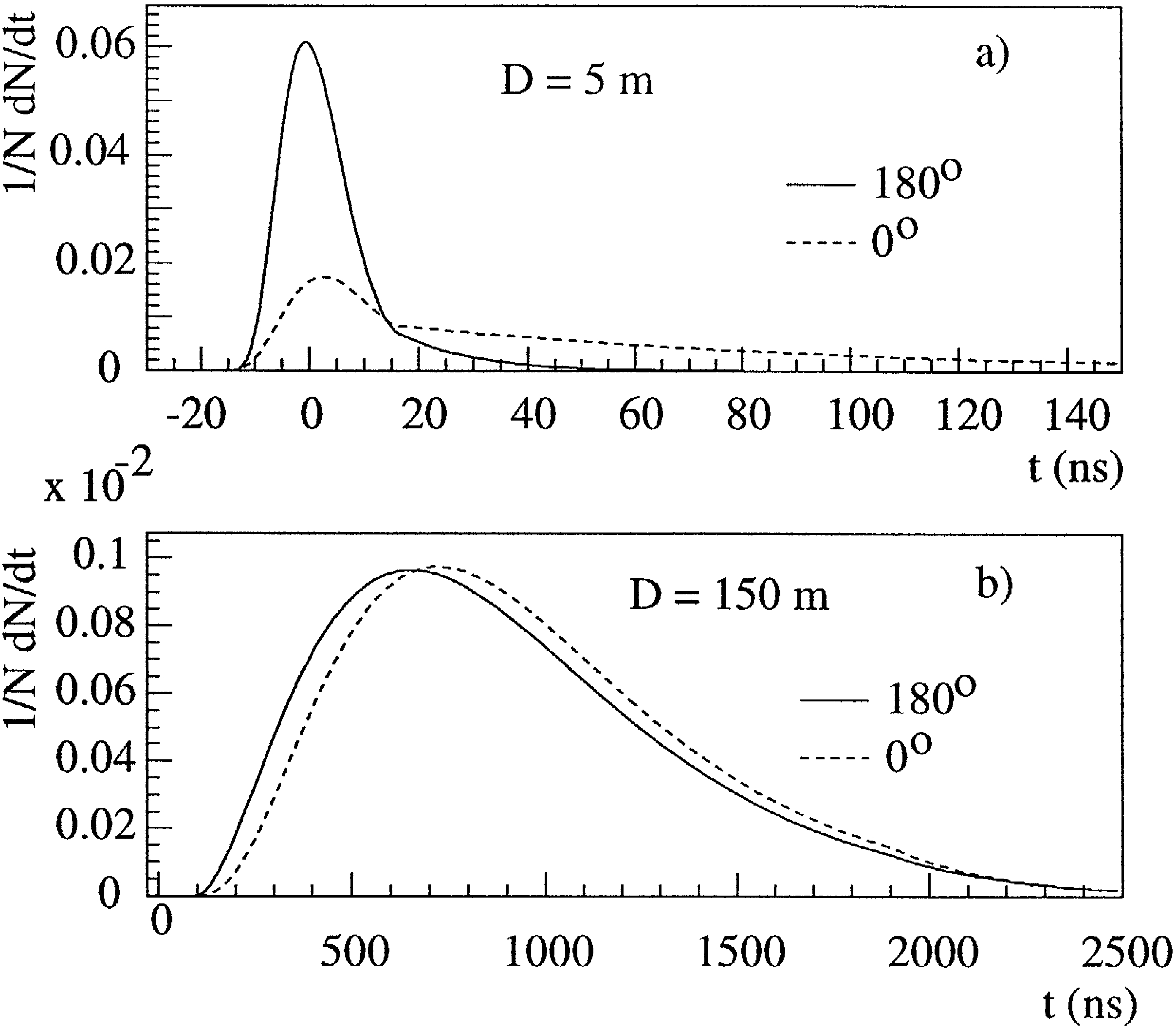
has a long tail at the high side – see Fig. 11.
To cope with the nonGaussian timing distribu
tions we used a likelihood analysis. In this approach,
.
a normalized probability distribution function
pt
i
gives the probability of a certain time delay
t
for a
.
Fig. 11. Delaytime distributions for modules facing full curves
.
and backfacing dashed curves a muon track. Data are shown for
. .
muon tracks with impact parameters of a 5 meters and b 150
meters.
given hit
i
with respect to straightly propagating
photons. This probability function is derived from
the MC simulations based on the photon propagation
tables introduced in Section 6.1. The probability
depends on the distance and the orientation of the
PMT with respect to the muon track. By varying the
track parameters the logarithm of a likelihood func
tion
L
L
is maximized.
log
L
L
s
log
p
s
log
p
.
. .
ii
/
all hits
all hits
In order to be used in the iteration process, the
time delays as obtained from the separate photon
propagation Monte Carlo have to be parameterized
by an analytic formula. The parameterization of the
propagation model itself is extended to allow for
timing errors of PMTs and electronics as well as the
probability of noise hits at random times. The
AMANDA collaboration has developed two inde
pendent reconstruction programs, which are based on
different parameterizations of the photon propagation
wx
and different minimization methods 26,27,29 . The
comparison of these algorithms and the use of differ
ent optical models show that the results of both
methods are in good agreement with each other and
do not depend on a finetuning of the assumed
optical parameters. Fig. 11 shows the result of the
parameterization of the time delay for two distances
and for two angles between the PMT axis and the
muon direction. At a distance of 5 m and a PMT
()
E. Andres et al.
r
Astroparticle Physics 13 2000 1–20
12
facing toward the muon track, the delay curve is
dominated by the time jitter of the PMT. However, if
the PMT looks in the opposite direction, the contri
bution of scattered photon yields a long tail towards
large delays. At distances as large as 150 m, distribu
tions for both directions of the PMT are close to
each other since all photons reaching the PMT are
multiply scattered.
The parameterization used for most of the results
presented in this paper is a Gamma distribution
wx
modified with an absorption term 28 ,
t
y
d
r
l
.
P
t
d
r
l
y
1
.
pd
,
t
s
N
P
.
G
d
r
l
.
P
e
y
t
r
t
q
c
w
P
t
r
X
0
q
d
r
X
0
,
with the distance
r
between OM and muon track, the
.
scaled distance
d
f
0.8
r
sin
u
P
r
, the absorption
c
length
X
and only two parameters
t
f
7001 ns and
0
l
f
50 m.
The second approach uses an Fdistribution with
an exponential tail for large timedelays, which re
wx
sults in a comparable accuracy 26 .
6.4. Quality analysis
Quality criteria are applied in order to select
events which are ‘‘well’’ reconstructed. The criteria
define cuts on topological event parameters and ob
servables derived from the reconstruction. Below we
list those used in the following:
<<
fl
Speed
z
of the line fit. Values close to the speed
of light indicate a reasonable pattern of the mea
sured times, values smaller than 0.1 m
r
nsec indi
cate an obscure time pattern.
.
fl
‘‘Time’’ likelihood per hit PMT log
L
L
r
N
.
time hit
fl
Summed hit probability for all hit PMTs
P
.
hit
fl
‘‘Hit’’ likelihood normalized to all working chan
.
nels, log
L
L
r
N
.
hit all
The latter two parameters are good indicators of
whether the location of the fitted track, which
relies exclusively on the time information, is
compatible with the location of the hits and non
hits within the detector.
fl
Number of direct hits,
N
, which is defined to be
dir
the number of hits with time residuals
t
mea
i
. .
sured
y
t
fit smaller than a certain cut value.
i
We use cut values of 15 nsec, 25 nsec and 75
nsec, and denote the corresponding parameters as
. . .
N
15 ,
N
25 and
N
75 , respectively. In
dir dir dir
creasing the time window leads to higher cut
values in
N
but allows a finer gradation of the
dir
cut.
Events with more than a certain minimum num
ber of direct hits i.e. only slightly delayed pho
.
tons are likely to be well reconstructed. This cut
wx
turned out to be the most powerful cut of all 29 .
fl
The projected length of direct hits onto the recon
structed track,
L
. A cut in this parameter rejects
dir
events with a small lever arm.
fl
Vertical coordinate of the center of gravity,
z
.
COG
Cuts on this parameter are used to reject events
close to the borders of the array. Very distant
tracks are not likely to be well reconstructed.
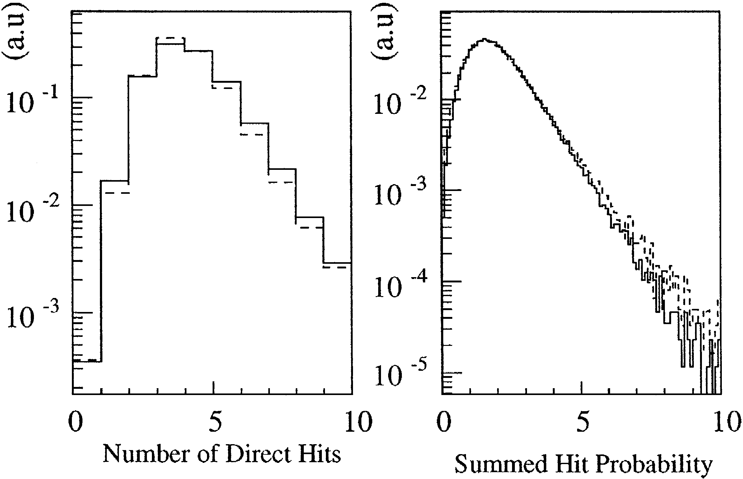
Fig. 12 shows the distribution of two of these
observables, the number of direct hits within 15
.
nsec,
N
15 , and the summed hit probability
P
dir hit
of all hit channels. It demonstrates the good agree
ment between results from MC and experiment.
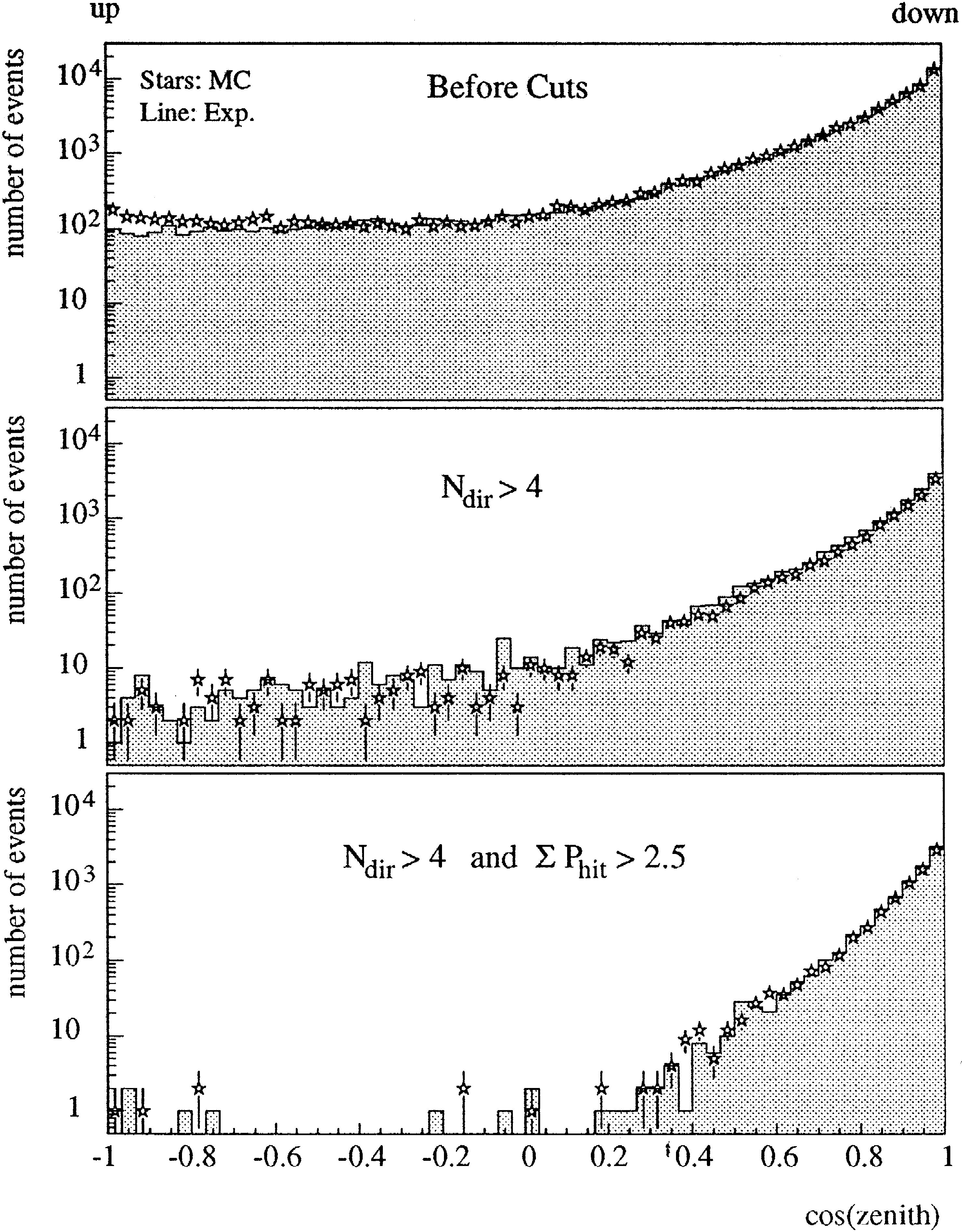
Fig. 13 demonstrates the effect of cuts on the
number of direct hits and the summed hit probability
on the reconstructed angular distribution of experi
mental data and the MC sample. The cuts are
.
N
15
G
5 and
P
G
2.5. Both samples are
direct hit
dominantly due to downgoing atmospheric muons.
Despite that, a small but similar fraction of events is
falsely reconstructed as upgoing events. After appli
cation of the above quality criteria the tail below the
horizon almost disappears. Note that not only the
Fig. 12. Distributions of two reconstructed event observables for
.
MC downgoing muon events dashed lines and from experimen
. .
tal data full lines . Left: Number of direct hits,
N
15 ; Right:
dir
summed hit probability,
P
.
hit
()
E. Andres et al.
r
Astroparticle Physics 13 2000 1–20
13
Fig. 13. Reconstructed zenith angle distributions of experimental
. .
data line and downward muon MC events points after a
stepwise application of quality cuts.
shapes but also the absolute passing rates on all cut
levels are in good agreement between data and Monte
Carlo. The angular mismatch between the recon
structed muon angle and the original angle used in
the MC simulation after both cuts is 5.5 degrees. We
note that this value strongly depends on the particu
lar set of cuts, the minimum acceptable passing rate,
the incident angle of the muon, and the range of
muons stopping in the array.
7. SPASE coincidences
AMANDA is unique in that it can be calibrated
by muons with known zenith and azimuth angles
which are tagged by air shower detectors at the
surface. AMANDAB4 has been running in coinci
dence with the two SPASE South Pole Air Shower
.
wx
Experiment arrays, SPASE1 34 and SPASE2
wx
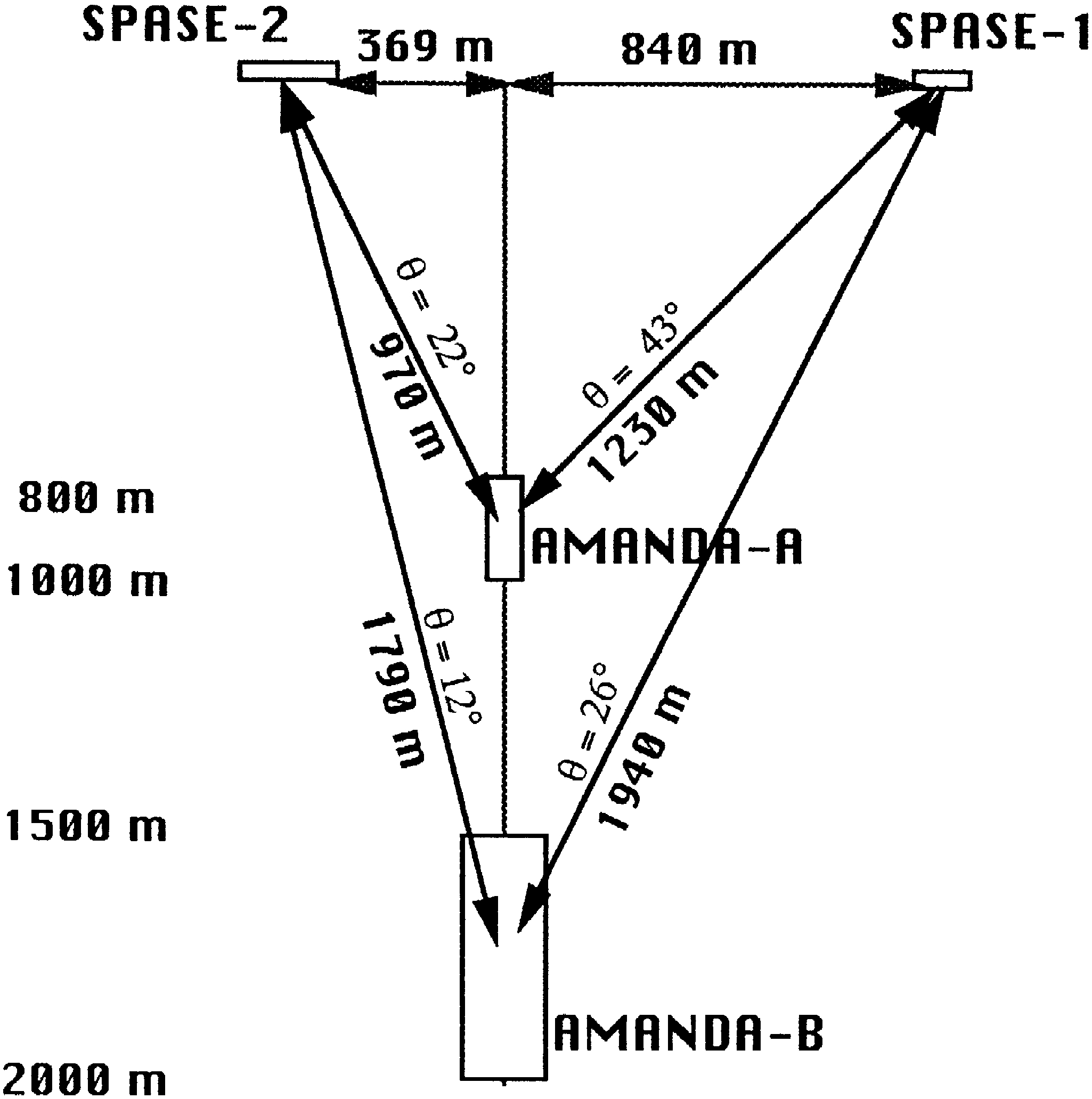
35 . SPASE1 was located 840 m from the center of
the AMANDA array projected to the surface, whereas
.
SPASE2 is located 370 m away see Fig. 14 . The
scintillation detectors of SPASE2 are complemented
wx
by an array of air Cherenkov detectors 31,32 . The
primary goal of these devices is the investigation of
the chemical composition of primary cosmic rays in
wx
the region of the ‘‘knee’’ 33 . Another detector, the
gamma imaging telescope GASP, is also operated in
coincidence with AMANDA.
In this section, we summarize calibration results
obtained from the coincident operation of AMANDA
and SPASE2. SPASE2 consists of 30 scintillator
stations of 0.8 m
2
on a 30 m triangular grid. The
area of the array is 1.6
P
10
4
m
2
, and it has been
running since January 1996. For each air shower, the
direction, core location, shower size and GPS time
are determined. Showers with sufficient energy to
.
trigger SPASE2
f
100 TeV yield on average 1.2
muons penetrating to the depth of AMANDAB. On
every SPASE1 or SPASE2 trigger, a signal is sent
to trigger AMANDA. The GPS times of the separate
events are compared offline to match coincident
events.
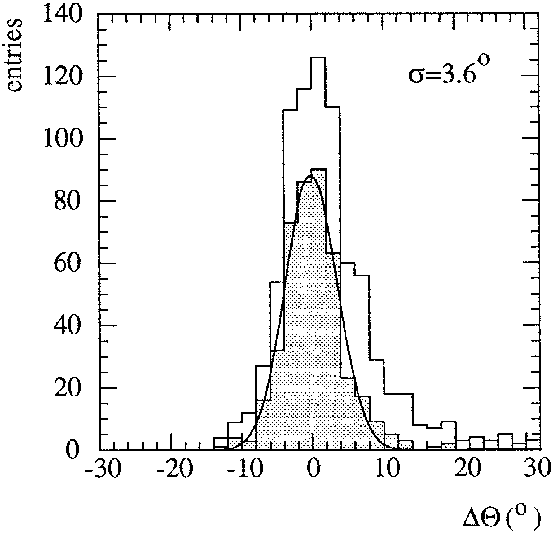
A oneweek sample of these events has been
analyzed in order to compare the directions of muons
determined by AMANDAB4 to those of the show
ers measured by SPASE2. A histogram of the zenith
mismatch angle between SPASE2 and AMANDA
B4 is shown in Fig. 15. The selected events are
required to have
G
8 hits along 3 strings and to yield
a track which is closer than 150 m to the air shower
.
axis measured by SPASE2 upper histogram . The
hatched histogram shows the distribution of the zenith
Fig. 14. Side view of the two SPASE arrays relative to
AMANDAA and AMANDAB.
()
E. Andres et al.
r
Astroparticle Physics 13 2000 1–20
14
Fig. 15. Mismatch between zenith angles determined in
AMANDAB4 and SPASE2.
mismatch angle after application of the following
quality cuts:
.
fl
likelihood log
L
L
r
N
)
y
12,
time hit
fl
more than four hits with residuals smaller than 75
. .
nsec
N
75
)
4,
dir
fl
length of the projection of OMs with direct hits to
. .
the track larger than 50 meters
L
75
)
50 m .
dir
428 of the originally 840 selected events pass
these quality cuts. The Gaussian fit has a mean of
.
0.14
"
0.19 degrees and a width of
s
s
3.6
"
.
0.17 degrees. This is nearly 2 degrees better than
the resolution obtained in the previous section for
all
downward muons and for a different set of cuts. MC
yields a resolution of about 4 degrees.
The small mean implies that there is little system
atic error in zenith angle reconstruction. The SPASE
2 pointing accuracy, which contributes to the average
mismatch, depends on zenith angle and shower size.
For most of the coincidence events, the SPASE2
pointing resolution, defined as the angular distance
within which 63% of events are contained, is be
wx
tween 1
8
and 2
8
31,32 .
8. Intensityvsdepth relation for atmospheric
muons
8.1. Angular dependence of the muon flux
In Section 6, the muon angular distribution was
shown as a function of various cuts in order to
demonstrate the agreement between experimental
data and MC simulations. In this section, we calcu
late the muon intensity
I
as a function of the zenith
.
angle
u
.
I
u
is given by
m
SN
u
P
m
u
.
.
dead
mm
I
u
s
,3
.
.
m
T
P
DVe u
P
A
cut,
u
. .
rec
m
eff
m
where
.
fl
N
u
is the number of muons assigned by the
m
analysis to a zenith angle interval centered around
cos
u
. For the analysis presented in this section,
m
.
we start from the angular distribution
N
u
m
rec
obtained from the reconstruction, without apply
ing cuts. This distribution is strongly smeared
.
see Fig. 13, top . We have calculated the ele
.
ments of the parent angular distribution
N
u
m
.
from the reconstructed distribution
N
u
using
m
rec
wx
a regularized deconvolution procedure 36,37 .
fl
T
is the runtime. We used the data from June 24,
1996, with
T
s
22.03 hours, and 9.86
P
10
5
events
triggering AMANDAB4.
fl
S
corrects for the dead time of the data acqui
dead
sition system. This factor was determined from
the time difference distribution of subsequent
events. The deadtime losses for the two runs
used in this analysis are 12%, i.e.
S
s
1
r
0.88
dead
s
1.14.
fl
DV
is the solid angle covered by the correspond
ing cos
u
interval.
m
.
fl
A
cut,
u
is the effective area, after the applica
eff
m
tion of a multiplicity trigger, for a given cut at
zenith angle
u
. The effective area is shown in
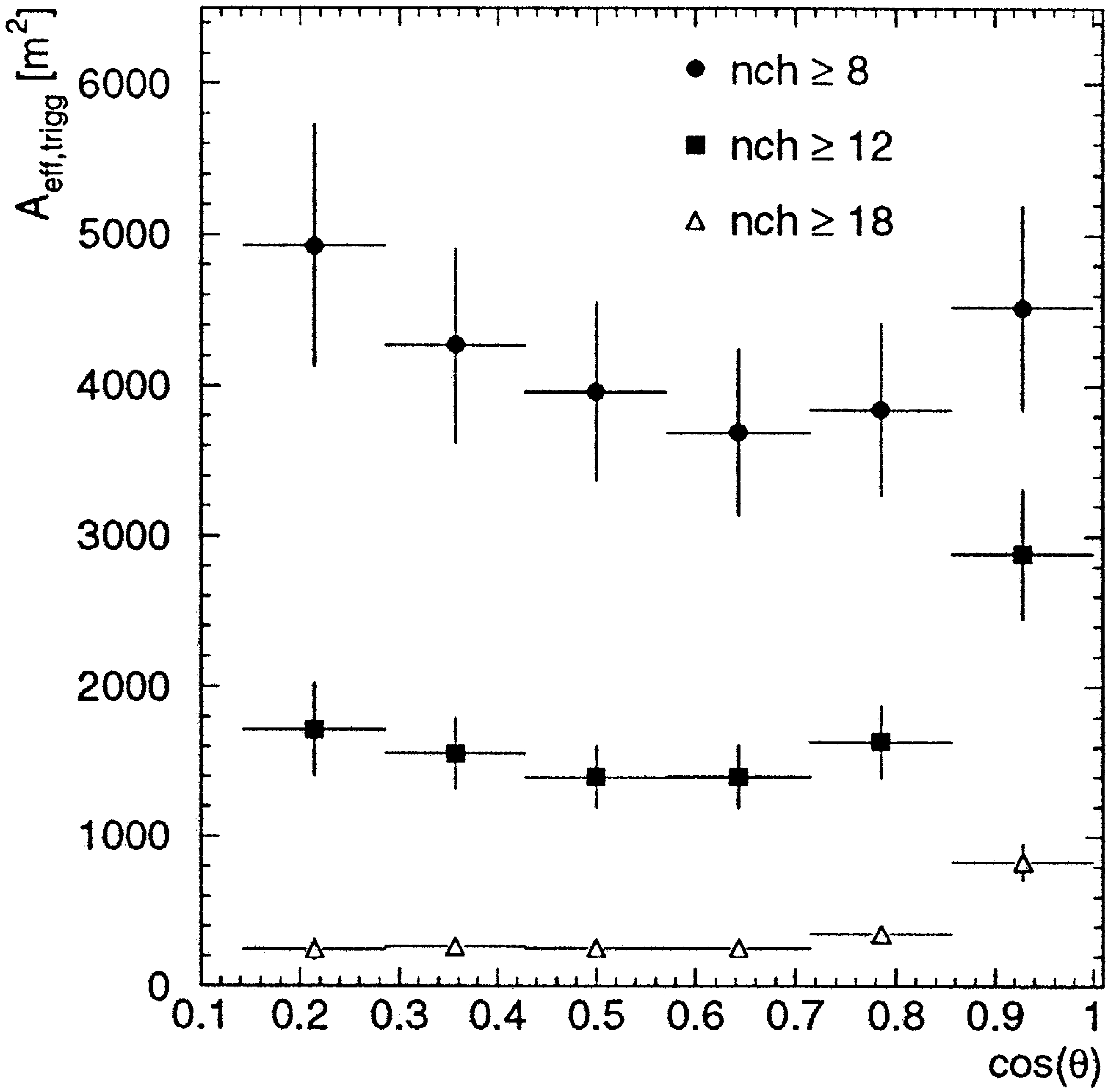
m
Fig. 16 as a function of the zenith angle and for
different cuts on the number of hit OMs.
.
fl
eu
is the reconstruction efficiency for zenith
rec
m
angle
u
which ranges between 0.82 at cos
u
s
1.0
m
and 0.75 at cos
u
s
0.2.
.
fl
m
u
is the mean muon multiplicity at angle
u
m
m
at the ‘‘trigger depth’’. The trigger depth
h
was
eff
defined as depth of
z
, the center of gravity in
OM
the vertical coordinate
z
of all hit OMs. The
average
h
depends on the angle. It is highest
eff
for cos
u
between 0.4 and 0.8 about 30 m below
.
the detector center and falls toward the vertical
.
at maximum 80 m below the center . The mean
muon multiplicity is about 1.2 for vertical tracks
and decreases towards the horizon. Since the
wx
generator used in this analysis 20 simulates only
()
E. Andres et al.
r
Astroparticle Physics 13 2000 1–20
15
Fig. 16. Effective trigger area of AMANDAB4 as a function of
zenith angle, for 3 different majority criteria.
proton induced showers, this value is an underes
timation by about 10%.
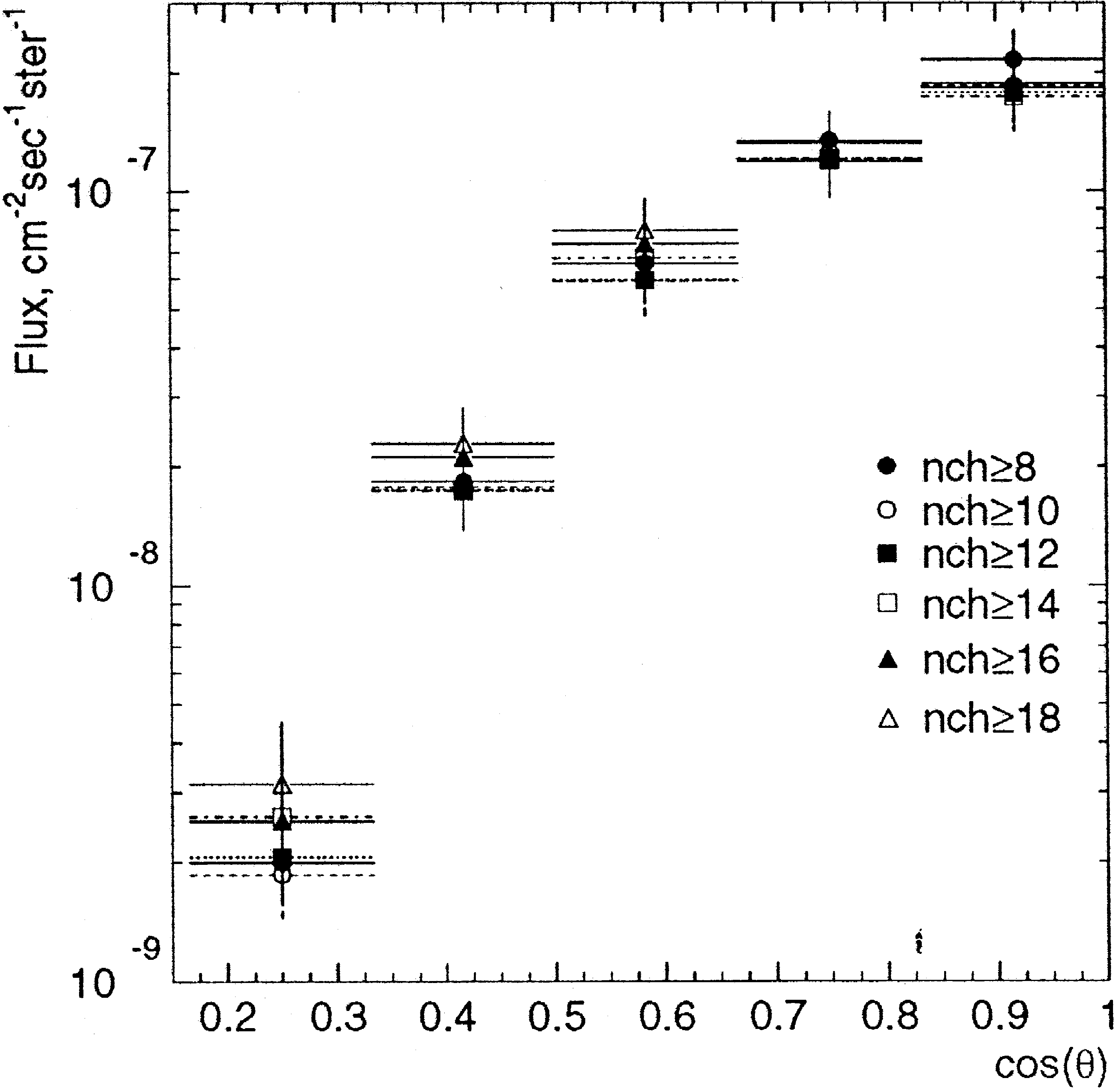
Fig. 17 shows the angular distribution of the flux
.
of downgoing muons,
I
u
, as obtained from Eq.
m
.
3 . In order to illustrate the stability of the method
with respect to cuts biasing the measured angular
distribution, the flux is shown for samples defined by
different majority triggers
N
)
8, 10, 12, 14, 16,
hit
.
18 . Apart from the point closest to the horizon
which is not only most strongly biased but also has
Fig. 17. Angular distribution of the downward going muon flux,
. .
I
u
, as obtained from Eq. 3 .
m
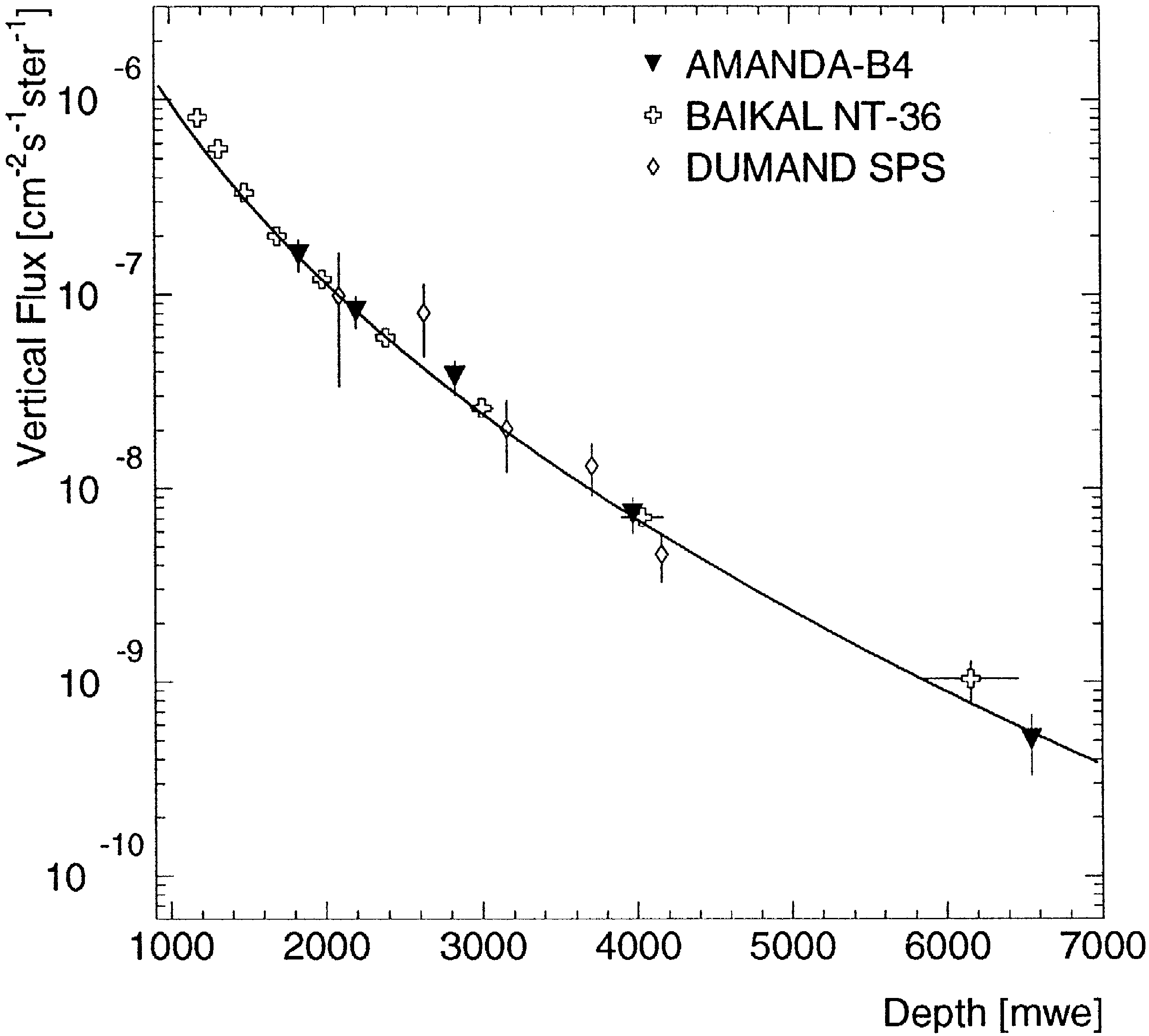
Fig. 18. Vertical intensity versus depth for AMANDA, BAIKAL
wx
and DUMAND. The solid line gives the prediction of 38 which
.
coincides with the curves obtained from the parameterizations 5
.
and 6 .
the lowest statistics, deviations are within 25%. For
further studies we use the sample with
N
G
16.
hit
8.2. Transformation of angular flux to
˝
ertical inten
sity as a function of depth
.
The measured flux
I
u
can be transformed into a
.
vertical flux
I
u
s
0,
h
, where
h
is the ice thickness
seen under an angle
u
,
I
u
s
0,
h
s
I
u
P
cos
u
P
c
4
. . . .
corr
.
The cos
u
conversion correcting for the sec
u
behavior of the muon flux is valid for angles up to
wx wx
60
8
46 . The term
c
taken from 44 corrects for
corr
larger angles and lies between 0.8 and 1.0 for the
angular and energy ranges considered here.
The vertical intensities obtained in this way are
plotted in Fig. 18 and compared to the depthinten
wx
sity data published by DUMAND 45 and Baikal
wx w x
7 , and to the prediction by Bugaev et al. 38 . One
observes satisfying agreement of all experiments with
the prediction.
We also fitted our data to a parameterization
wx
taken from 39,40 ,
Ih
s
I
P
E
y
g
.
0crit
y
g
a
b
P
h
.
eff
wx
s
I
PP
e
y
1. 5
.
0
/
b
eff
()
E. Andres et al.
r
Astroparticle Physics 13 2000 1–20
16
E
is the minimum energy necessary to reach
crit
the depth
h
. It is obtained from the parameterization
wx
46
dE
r
dx
s
a
q
b
P
E
where
a
f
2 MeV
r
g
P
m
y
2
.
cm denotes the continuous energy loss due to
.
ionization, and
bE
is proportional to the stochas
m
tic energy loss due to pair production, bremsstrahlung
and nuclear cascades. From this parameterization one
w
.
x
obtains
E
s
a
r
b
P
exp
b
P
h
y
1.
I
is the nor
crit 0
wx
malization parameter and
g
f
2.78 40 the spectral
.
index. We approximate
bE
by an energy indepen
m
.
dent parameter
b
. Fitted to Eq. 5 , our data for the
eff
vertical intensity result in the following values for
I
0
and
b
:
eff
I
s
5.04
"
0.13 cm
y
2
s
y
1
ster
y
1
,
.
0
b
s
2.94
"
0.09
P
10
y
6
g
y
1
cm
2
.
.
eff
.
y
2
y
1
This compares to
I
s
5.01
"
0.01 cm s
0
y
1
.
y
6
y
12
ster and
b
s
3.08
"
0.06 10 g cm ob
eff
tained for
N
G
8, showing that the result is rather
hit
insensitive to the actual cut condition.
For the purpose of completeness we give also the
results for the more usual parameterization,
a
l
y
h
r
l
Ih
,
u
s
0
s
a
e, 6
.
.
m m
/
h
wx wx
where
a
is set to 0 41 , to 2 42 or is a free
wx
parameter 43 . The purely exponential dependence
.
a
s
0 clearly does not describe the data at depths
smaller than 4–5 km. Leaving all parameters free
wx
.
y
6
y
2
43 , one obtains
a
s
0.89
"
0.30
P
10 cm
m
y
1
y
1
.
y
2
s ster ,
l
s
1453
"
612 g cm , and
a
s
2.0
"
0.25, being also in agreement with
a
fixed as in
wx
Ref. 42 .
9. Search for upward going muons
AMANDAB4 was not intended to be a full
fledged neutrino detector, but instead a device which
demonstrates the feasibility of muon track recon
struction in Antarctic ice. The limited number of
optical modules and the small lever arms in all but
the vertical direction complicate the rejection of fake
events. In this section we demonstrate that in spite of
that the separation of a few upward muon candidates
was possible.
We present the results of two independent analy
ses. One uses the approximation of the likelihood
function by a Ffunction with an exponential tail
wx
26 , the other the approximation by a Gamma func
wx
.
tion with an absorption term 27 see Section 6.3 .
Both analyses apply separation criteria which are
obtained from a stepwise tightening of cuts on differ
ent parameters, in a way which improves the signal
tofake ratio given by the MC samples. Since the
MC generated samples of downwardgoing muons a
.
few million events run out of statistics after a
reduction factor of about 10
6
, further tightening of
cuts is performed without backgroundMC control
until the experimental sample reaches the same mag
nitude as the MC predicted signal.
For both analyses, the full experimental data set
of 1996, starting with Feb. 19th and ending with
Nov. 5th, was processed. It consists of 3.5
P
10
8
events.
9.1. Analysis 1
In a first step, a fast prefilter reduced this sample
to a more manageable size. It consists of a number of
cuts on quickly computable variables which either
correlate with the muon angle, or which to a certain
degree distinguish single muons from the downgoing
multimuon background events like, e.g. a cut on the
wx
zenith angle from a line fit 25 , cuts on time differ
ences between OMs at different vertical positions,
and topological cuts requesting a minimum vertical
elongation of the event.
These cuts reduce the size of the experimental
data sample to 5.2%, the simulated atmospheric
muons to 4.8% and simulated upgoing events to
49.8%.
Simulated upgoing events and experimental data
have been reduced by further cuts,
fl
At least 2 strings have to be hit this condition
relaxes the standard condition ‘‘
G
3 strings’’ and
increases the effective area in the vertical direc
.
tion .
fl
The events were reconstructed below horizon, i.e.
u
)
90
8
.
.
fl
log
L
L
r
N
)
y
6.
time hit
fl
a
G
0.15 m
r
nsec, where
a
is obtained from a fit
to
z
s
a
P
t
q
b
and
z
,
t
being the
z
coordi
ii i i
nates and times of the hit OMs.
()
E. Andres et al.
r
Astroparticle Physics 13 2000 1–20
17
Fig. 19. Number of events surviving prefilter and additional cuts
.
as a function of
N
15 . Solid line: 6month experimental data.
dir
dashed line: 6month expectation from atmospheric neutrinos.
Fig. 19 shows the distribution of the number of
.
direct hits,
N
15 , of all events passing these cuts.
dir
The highest cut in
N
survived by
any
experi
direct
mental event is
N
G
6. The two surviving events
direct
are shown in Fig. 20. The Monte Carlo expectation
for upward muons from atmospheric neutrinos is 2.8
events, with an uncertainty of a factor 2, mostly due
to uncertainties in the sensitivity of the detector after
all cuts.
9.2. Analysis 2
The 3.5
P
10
8
experimental events were compared
to 3.5
P
10
6
MC events from atmospheric downgoing
muons which correspond to 2 days effective line
time. The MC data set for upward muons from
wx
atmospheric neutrino interactions 47 consists of
2.5
P
10
3
events triggering AMANDAB4 – corre
sponding to 1.7 years effective live time.
In order to separate neutrino induced upward
muons, we applied a number of successively tight
ened cuts in the variables defined in Section 6.4.
This procedure reduced the experimental sample to
the expected signal sample after the following cuts:
1. reconstructed zenith angle
u
)
120
8
,
<<
2. speed of the line fit 0.15
z
1m
r
nsec,
. .
3. ‘‘time’’ likelihood log
L
L
r
N
y
5
)
y
10
time hit
i.e. normalizing to the degrees of freedom in
.
stead of the number of hit PMTs ,
. .
4. ‘‘hit’’ likelihood log
L
L
r
N
y
5
)
y
8,
hit hit
5. number of direct hits for 25 nsec window,
.
N
25
G
5,
dir
6. number of direct hits for 75 nsec window,
.
L
25
)
200 m,
dir
7. absolute value of the vertical coordinate of the
<<
center of gravity
z
90 m with the center
COG
of the detector defining the origin of the coordi
.
nate system .
Three events of the experimental sample passed
these cuts, corresponding to a suppression factor of
8.9
P
10
y
9
. The passing rate for MC upward moving
muons from atmospheric neutrinos is 1.3% which
corresponds to 4.0 events in 156 days. The corre
y
9
sponding enrichment factor is 0.013
r
8.9
P
10
f
1.5
P
10
6
. One of the three experimental events was
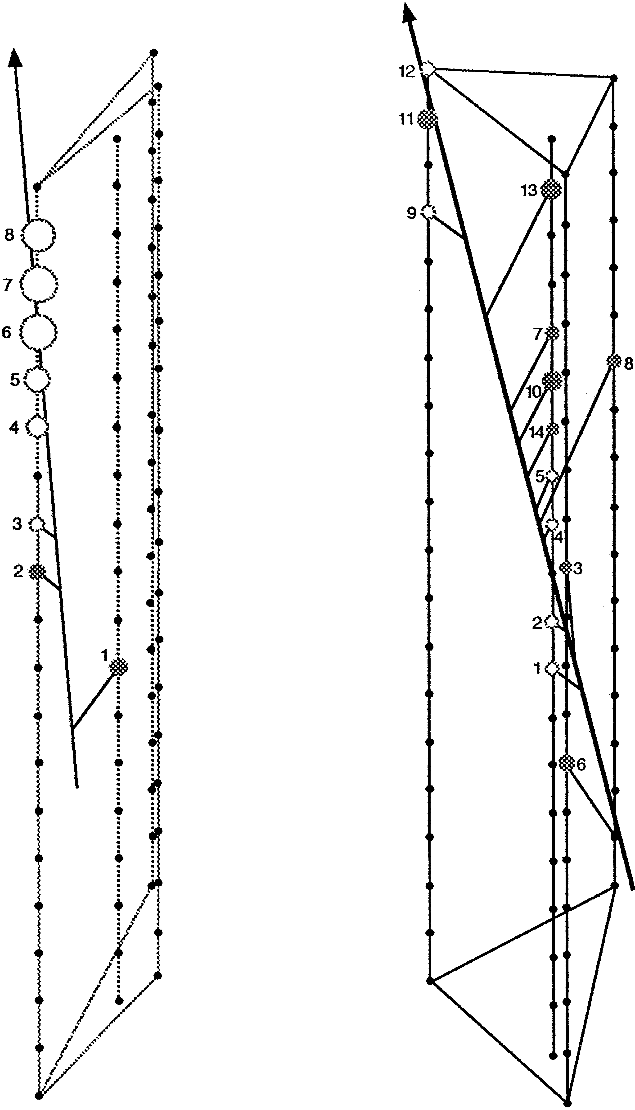
Fig. 20. The two experimental events reconstructed as upward
muons, left: ID 8427997, right: ID 4706870. The line with an
arrow symbolizes the fitted muon track, the lines from this track
to the OMs indicate light pathes. The amplitudes are proportional
to the size of the OMs. The numbering of the OMs refers to the
time order in which they are hit.
()
E. Andres et al.
r
Astroparticle Physics 13 2000 1–20
18
identified also in the search from the previous sub
section. A second event with
N
s
5 passes all cuts
dir
of the previous analysis, with the exception of the
N
cut.
dir
In order to check how well the parameter distribu
tions of the events agree with what one expects for
atmospheric neutrino interactions, and how well they
are separated from the rest of the experimental data,
.
we relaxed two cuts at a time retaining the rest and
inspected the distribution in the two ‘‘free’’ vari
ables.
.
Fig. 21 shows the distribution in
L
25 and
dir
.
N
75 . The three events passing
all
cuts are sepa
dir
rated from the bulk of the data. At the bottom of Fig.
21, the data are plotted versus a combined parameter,
. . .
S
s
N
75
y
2
P
L
25
r
20. In this parameter,
dir dir
. .
Fig. 21. Top – distribution in parameters
L
25 versus
N
75 ,
dir dir
.
bottom: distribution in the ‘‘combined’’ parameter
S
s
N
75
P
dir
.
L
25
r
20. The cuts applied to the event sample include all cuts
dir
with the exception of cuts 6 and 7.
<<
.
Fig. 22. Distribution in parameters
z
versus
L
25 , after appli
dir
cation of all cuts with the exception of cuts 2 and 7, which have
been relaxed. top: experimental data, bottom: signal Monte Carlo
sample.
the data exhibit a nearly exponential decrease. As
suming the decrease of the background dominated
events to continue at higher
S
values, one can calcu
late the probability that the separated events are fake
events. The probability to observe one event at
S
G
70 is 15%, the probability to observe 3 events is only
6
P
10
y
4
.
<<
Fig. 22 shows the distribution when
z
and
.
L
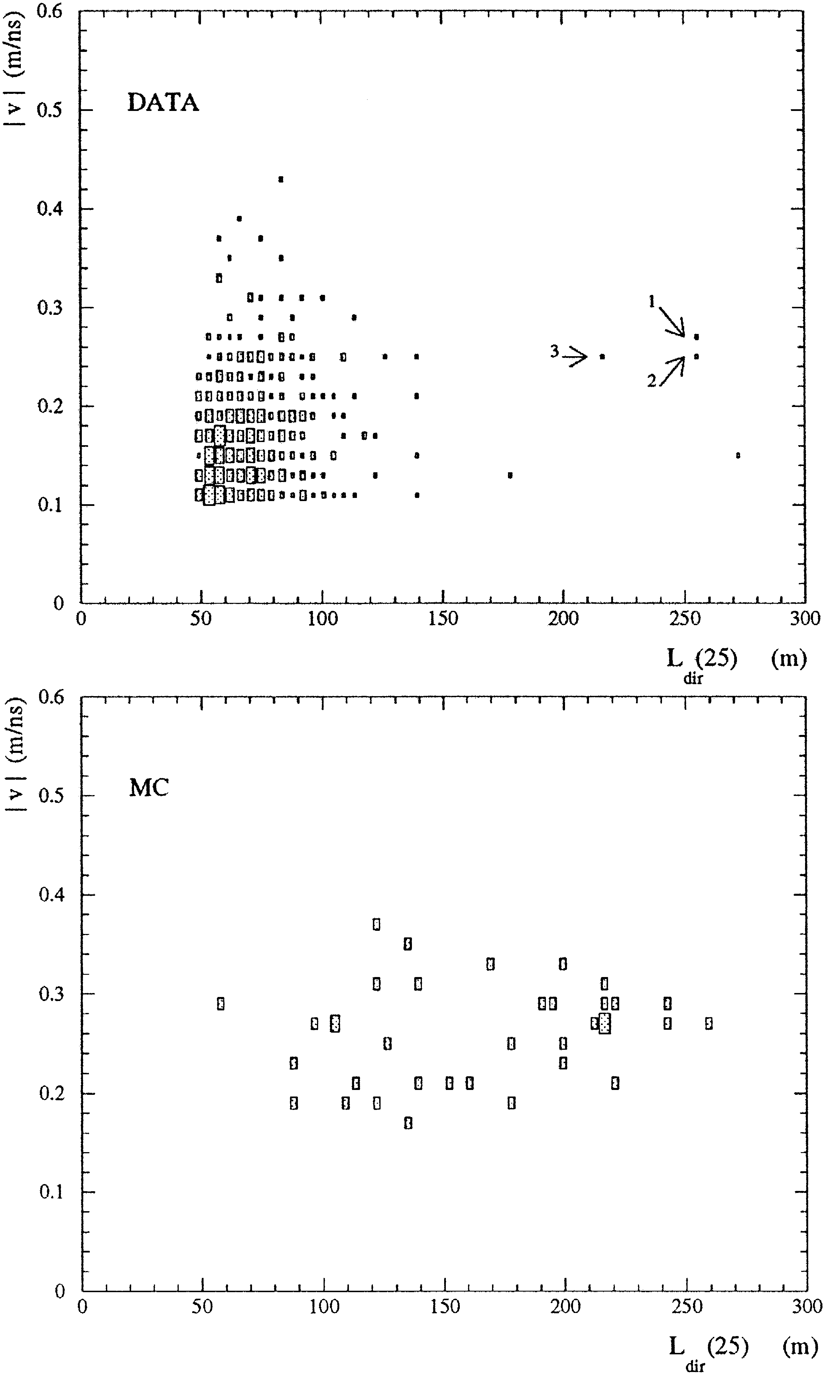
25 are relaxed. The 3 events are marked by
dir
.
arrows. There is one additional event at high
L
25 ,
dir
<<
which, however, has a somewhat too small
z
. The 3
events fall into the region populated by MC gener
ated atmospheric neutrino events passing the same
.
cuts bottom of Fig. 22 . We attribute the lack of
()
E. Andres et al.
r
Astroparticle Physics 13 2000 1–20
19
Table1
Characteristics of the events reconstructed as upgoing muons
Event ID
“
147742 4 706879 2 324428 8 427905
N
13 14 15 8
OM
N
34 3 2
string
..
log
L
r
N
y
5
y
8.3
y
8.5
y
8.0
y
11.2
hit
u
, degrees 168.7 165.9 166.7 175.4
rec
f
, degrees 45.8 274.2 194.1 –
rec
.
experimental events between
L
25
;
150–200 to
dir
statistical fluctuations.
Due to CPU limitation we could not check the
agreement between experimental data and atmo
spheric muon MC down to a 8.9
P
10
y
9
reduction.
However, down to a reduction of 10
y
5
, the disagree
ment does not exceed a factor of 3. A less conserva
tive estimate of the accuracy of the signal prediction
can be obtained by replacing all dedicated cuts for
u
)
90
8
by the complementary cuts for
u
90
8
.We
observed a betterthan10% agreement between ex
perimental data and MC after all cuts. In conclusion
we estimate the uncertainty in the prediction of
upward muon neutrinos to be about a factor 2.
Table 1 summarizes the characteristics of the
neutrino candidates identified in the two analyses.
We conclude that tracks reconstructed as upgoing
are found at a rate consistent with that expected for
atmospheric neutrinos. The three events found in the
second analysis are well separated from background
proving that, even with a detector as small as
AMANDAB4, neutrino candidates can be separated
within a limited zenith angle interval. Meanwhile, a
few tens of clear neutrino events have been identi
fied with the more powerful AMANDAB10 tele
scope. They will be the subject of a forthcoming
paper.
10. Conclusions
We have described the design, operation, calibra
tion and selected results of the prototype neutrino
telescope AMANDAB4 at the South Pole.
The main results can be summarized as follows:
fl
AMANDAB4 consisting of 80 optical modules
.
q
6 OMs for technology tests on 4 strings has
been deployed at depths between 1.5 and 2.0 km
in 1996. Seven of the OMs failed during refreez
ing. We have developed reliable drilling and in
strumentation procedures allowing deployment of
a 2 km deep string in less than a week. In the
mean time the detector has been upgraded to 302
. .
AMANDAB4, 1997 and 424 1998 optical
modules.
fl
The ice properties between 1.5 and 2.0 km are
superior to those at shallow depths. The absorp
tion length is about 95 m and the effective scatter
ing length about 24 m.
fl
The original calibration accuracy reached for ge
ometry and timing of AMANDAB4 was about 2
m and 7 nsec, respectively. With the upgrade to
10 strings, these values have been improved to
0.5–1.0 m and 5 nsec.
fl
We have developed proper methods for track
reconstruction in a medium with nonnegligible
scattering. With tailored quality cuts, the remain
ing badly reconstructed tracks can be removed.
The quality of the reconstruction and the effi
ciency of the cuts improve considerably with
increasing size of the array.
fl
Geometry and tracking accuracy of AMANDA
can be calibrated with surface air shower detec
tors. The mismatch between showers detected in
the SPASE air shower array and muons detected
with AMANDA is about 4 degrees, in agreement
with Monte Carlo estimates of the angular accu
racy.
fl
The measured angular spectrum of the intensity
of atmospheric muons is in good agreement with
other experiments and with model calculations.
fl
First neutrino candidates have been separated with
AMANDAB4. The identification of upward
muon candidates with an array of only 73 operat
ing 8inch PMTs is a demonstration that deep
antarctic ice is an adequate medium for doing
neutrino astronomy.
AMANDAB4 is a first step towards a large
neutrino telescope at the South Pole. A tenstring
array, AMANDAB10, has been taking data since
1997. Presently, B10 data are analyzed, and tens of
clear neutrino candidates have been extracted, with a
threshold of typically 50 GeV. The construction of
AMANDAII, a 30000 m
2
array, is underway. The
()
E. Andres et al.
r
Astroparticle Physics 13 2000 1–20
20
longterm goal of the collaboration is a cube kilome
ter detector, ICECUBE.
Acknowledgements
This research was supported by the U.S. National
Science Foundation, Office of Polar Programs and
Physics Division, the University of Wisconsin
Alumni Research Foundation, the U.S. Department
of Energy, the U.S. National Energy Research Scien
tific Computing Center, the Swedish Natural Science
Research Council, the Swedish Polar Research Sec
retariat, the Knut and Alice Wallenberg Foundation,
Sweden, and the Federal Ministery for Education and
Research, Germany. C.P.H. acknowledges the sup
port of the European Commission through TMR
contract No. ERBFMBICT91551.
We thank the Polar Ice Coring Office, PICO, for
bore hole drilling, and the Antarctic Support Associ
ates, ASA, as well as the staff of the Amundsen
Scott station for support and assistance. We grate
fully acknowledge help from the SPASE collabora
tion, Leeds University, and the U.K. Particle Physics
and Astrophysics Research Council.
References
wx
.
1 T. Gaisser, F. Halzen, T. Stanev, Phys. Rep. 258 1995 174.
wx
.
2 A. Bottino et al., Astropart. Phys. 2 1994 77.
wx
3 L. Bergstrom, J. Edsjo, astroph
r
9607237.
¨¨
wx
.
4 F. Halzen, J. Jacobsen, E. Zas, Phys. Rev. D 49 1994 1758.
wx
.
5 J.L. Thorn et al., Phys. Rev. D 46 1992 4846.
wx
6 Z. Djilkibaev, Proc. Int. Workshop on Simulation and Analy
sis Methods for Large Neutrino Telescopes, Zeuthen, Ger
.
many 1998 .
wx
.
7 I.A. Belolaptikov et al., Astropart. Phys. 7 1997 263.
wx
.
8 P. Askebjer et al., Science 267 1995 1147.
wx
.
9 AMANDA Collaboration, J. Glaciology 41 1995 445.
wx
.
10 Project Description Baikal 9203 DESY 1992 ; V. Balkanov
et al., astroph
r
9903342.
wx
.
11 DUMAND II Proposal HDC288 Hawaii, 1988 .
wx
.
12 S. Matsuno et al., Nucl. Instr. & Methods A 276 1989 359.
wx
13 L.K. Resvanis et al., Proc. High Energy Neutrino Astro
physics Workshop, Hawaii, X. Tata, ed. World Scientific,
.
Singapore, 1992 p. 325.
wx
14 ANTARES Proposal 1997; astroph
r
9707136.
wx
.
15 D.M. Lowder et al., Nature 353 1991 331.
wx
16 Yu.F. Barkov et al. Moscow Glaciological Research Publi
.
cation, 1984 .
wx
17 R. Wischnewski et al., Proc. 24th Int. Cosmic Ray Conf.,
.
Rome, Italy 1 1995 p. 658.
wx
18 R. Porrata et al., Proc. 25th Int. Cosmic Ray Conf., Durban,
.
South Africa 7 1997 237.
wx
19 D. Lowder, K. Woschnagg, Proc. Int. Workshop on Simula
tion and Analysis Methods for Large Neutrino Telescopes,
.
Zeuthen, Germany 1998 .
wx
20 S.N. Boziev et al., INR Preprint P0630 Moscow, Russia,
.
1989 .
wx
21 E. Scapparone, Proc. Int. Workshop on Simulation and Anal
ysis Methods for Large Neutrino Telescopes, Zeuthen, Ger
.
many 1998 , and references therein.
wx
.
22 L. Volkova, Sov. J. Nucl. Phys. 31 1980 784.
wx
.
23 W. Lohmann, R. Kopp, R. Voss, CERN 8503 1985 .
wx
24 S. Hundertmark, Proc. Int. Workshop on Simulation and
Analysis Methods for Large Neutrino Telescopes, Zeuthen,
.
Germany 1998 .
wx
25 V.J. Stenger, University of Hawaii, HDC190; see also J.
Jacobsen, PhD thesis, http:
rr
alizarin.physics.wisc.edu
r
jacobsen.
wx
26 A. Bouchta, PhD thesis, Stockholm 1998, USIP Report 9807.
wx
27 C. Wiebusch, Proc. Int. Workshop on Simulation and Analy
sis Methods for Large Neutrino Telescopes, Zeuthen, Ger
.
many 1998 .
wx
28 D. Pandel, Diploma thesis HumboldtUniversity Berlin,
.
1996 .
wx
29 C. Wiebusch et al., Proc. 25th Int. Cosmic Ray Conf.,
.
Durban, South Africa 7 1997 13.
wx
30 A. Biron et al., Upgrade of AMANDAB towards
AMANDAII, DESY PRC 97
r
05, http:
rr
www.ifh.de
r
amanda
r
publications
r
proposal.
wx
31 J. Dickinson et al., Proc. 25th Int. Cosmic Ray Conf.,
.
Durban, South Africa 5 1997 233.
wx
32 J. Dickinson et al., Proc. 25th Int. Cosmic Ray Conf.,
.
Durban, South Africa 5 1997 229.
wx
33 T. Miller et al., Proc. 25th Int. Cosmic Ray Conf., Durban,
.
South Africa 5 1997 237.
wx
.
34 J. Beaman et al., Phys. Rev. D 48 1993 4495.
wx
35 T.K. Gaisser et al., Proc. 24th Int. Cosmic Ray Conf., Rome,
.
Italy 1 1995 938.
wx
36 V. Blobel, Unfolding in High Energy Physics, DESY84118,
1984, and Regularized Unfolding for High Energy Physics
.
Experiments, Opal Note TN361 1996 .
wx
37 G. Zech, Comparing Statistical Date to Monte Carlo Simula
tion: Parameter Fitting and Unfolding, DESY95113 June
.
1995 .
wx
.
38 E. Bugaev et al., Phys. Rev. D 58 1998 .
wx
.
39 C. Allkover, Cosmic Rays on Earth Karlsruhe, 1984 .
wx
.
40 W. Rhode, PhD thesis, Wuppertal 1993 .
wx
.
41 M. Crouch et al., Phys. Rev. D 18 1978 2239.
wx
.
42 C. Berger et al., Phys. Rev. D 40 1989 2163.
wx
.
43 M. Ambrosio et al., Phys. Rev. D 52 1995 3793.
wx
.
44 P. Lipari, Astropart. Phys. 1 1993 1995.
wx
.
45 J. Babson et al., Phys. Rev. D 42 1990 41.
wx
46 T. Gaisser, Cosmic Rays and Particle Physics Cambridge
.
Univ. Press, Cambridge, 1990 .
wx
47 E. Dahlberg, USIP Report 9802, Stockholm 1997.
Back to top