Observation of high energy atmospheric neutrinos with the Antarctic muon
and neutrino detector array
J. Ahrens,
9
E. Andre
´
s,
14
X. Bai,
1
G. Barouch,
11
S. W. Barwick,
8
R. C. Bay,
7
T. Becka,
9
K.H. Becker,
2
D. Bertrand,
3
F. Binon,
3
A. Biron,
4
J. Booth,
8
O. Botner,
13
A. Bouchta,
4,
*
O. Bouhali,
3
M. M. Boyce,
11
S. Carius,
5
A. Chen,
11
D. Chirkin,
7
J. Conrad,
13
J. Cooley,
11
C. G. S. Costa,
3
D. F. Cowen,
10
E. Dalberg,
14,†
C. De Clercq,
15
T. DeYoung,
11,‡
P. Desiati,
11
J.P. Dewulf,
3
P. Doksus,
11
J. Edsjo
¨
,
14
P. Ekstro
¨
m,
14
T. Feser,
9
J.M. Fre
`
re,
3
T. K. Gaisser,
1
M. Gaug,
4,§
A. Goldschmidt,
6
A. Hallgren,
13
F. Halzen,
11
K. Hanson,
10
R. Hardtke,
11
T. Hauschildt,
4
M. Hellwig,
9
H. Heukenkamp,
4
G. C. Hill,
11
P. O. Hulth,
14
S. Hundertmark,
8
J. Jacobsen,
6
A. Karle,
11
J. Kim,
8
B. Koci,
11
L. Ko
¨
pke,
9
M. Kowalski,
4
J. I. Lamoureux,
6
H. Leich,
4
M. Leuthold,
4
P. Lindahl,
5
I. Liubarsky,
11
P. Loaiza,
13
D. M. Lowder,
7,
i
J. Madsen,
12
P. Marciniewski,
13,¶
H. S. Matis,
6
C. P. McParland,
6
T. C. Miller,
1,
**
, Y. Minaeva,
14
P. Mioc
ˇ
inovic
´
,
7
P. C. Mock,
8,††
R. Morse,
11
T. Neunho
¨
ffer,
9
P. Niessen,
4,15
D. R. Nygren,
6
H. O
¨
gelman,
11
Ph. Olbrechts,
15
C. Pe
´
rez de los Heros,
13
A. C. Pohl,
5
R. Porrata,
8,‡‡
P. B. Price,
7
G. T. Przybylski,
6
K. Rawlins,
11
C. Reed,
8,§§
W. Rhode,
2
M. Ribordy,
4
S. Richter,
11
J. Rodrı
´
guez Martino,
14
P. Romenesko,
11
D. Ross,
8
H.G. Sander,
9
T. Schmidt,
4
D. Schneider,
11
R. Schwarz,
11
A. Silvestri,
2,4
M. Solarz,
7
G. M. Spiczak,
12
C. Spiering,
4
N. Starinsky,
11,
ii
D. Steele,
11
P. Steffen,
4
R. G. Stokstad,
6
O. Streicher,
4
P. Sudhoff,
4
K.H. Sulanke,
4
I. Taboada,
10
L. Thollander,
14
T. Thon,
4
S. Tilav,
1
M. Vander Donckt,
3
C. Walck,
14
C. Weinheimer,
9
C. H. Wiebusch,
4,
*
C. Wiedeman,
14
R. Wischnewski,
4
H. Wissing,
4
K. Woschnagg,
7
W. Wu,
8
G. Yodh,
8
and S. Young
8
~
AMANDA Collaboration
!
1
Bartol Research Institute, University of Delaware, Newark, Delaware 19716
2
Fachbereich 8 Physik, BUGH Wuppertal, D42097 Wuppertal, Germany
3
Universite
´
Libre de Bruxelles, Science Faculty CP230, Boulevard du Triomphe, B1050 Brussels, Belgium
4
DESYZeuthen, D15735 Zeuthen, Germany
5
Department of Technology, Kalmar University, S39182 Kalmar, Sweden
6
Lawrence Berkeley National Laboratory, Berkeley, California 94720
7
Department of Physics, University of California, Berkeley, California 94720
8
Department of Physics and Astronomy, University of California, Irvine, California 92697
9
Institute of Physics, University of Mainz, Staudinger Weg 7, D55099 Mainz, Germany
10
Department of Physics and Astronomy, University of Pennsylvania, Philadelphia, Pennsylvania 19104
11
Department of Physics, University of Wisconsin, Madison, Wisconsin 53706
12
Physics Department, University of Wisconsin, River Falls, Wisconsin 54022
13
Division of High Energy Physics, Uppsala University, S75121 Uppsala, Sweden
14
Department of Physics, Stockholm University, SCFAB, SE10691 Stockholm, Sweden
15
Vrije Universiteit Brussel, Dienst ELEM, B1050 Brussel, Belgium
~
Received 1 February 2002; published 31 July 2002
!
The Antarctic muon and neutrino detector array
~
AMANDA
!
began collecting data with ten strings in 1997.
Results from the first year of operation are presented. Neutrinos coming through the Earth from the Northern
Hemisphere are identified by secondary muons moving upward through the array. Cosmic rays in the atmo
sphere generate a background of downward moving muons, which are about 10
6
times more abundant than the
upward moving muons. Over 130 days of exposure, we observed a total of about 300 neutrino events. In the
same period, a background of 1.05
3
10
9
cosmic ray muon events was recorded. The observed neutrino flux is
consistent with atmospheric neutrino predictions. Monte Carlo simulations indicate that 90% of these events lie
in the energy range 66 GeV to 3.4 TeV. The observation of atmospheric neutrinos consistent with expectations
establishes AMANDAB10 as a working neutrino telescope.
DOI: 10.1103/PhysRevD.66.012005 PACS number
~
s
!
: 95.85.Ry, 95.55.Vj, 96.40.Tv
*
Now at CERN, CH1211, Gene
`
ve 23, Switzerland.
†
Now at Defense Research Establishment
~
FOA
!
, S17290 Stockholm, Sweden.
‡
Now at Santa Cruz Institute for Particle Physics, University of California—Santa Cruz, Santa Cruz, CA 95064.
§
Now at IFAE, 08193 Barcelona, Spain.
i
Now at MontaVista Software, 1237 E. Arques Ave., Sunnyvale, CA 94085.
¶
Now at The Svedberg Laboratory, S75121 Uppsala, Sweden.
**
Now at Johns Hopkins University, Applied Physics Laboratory, Laurel, MD 20723.
††
Now at Optical Networks Research, JDS Uniphase, 100 Willowbrook Rd., Freehold, NJ 077282879.
‡‡
Now at L174, Lawrence Livermore National Laboratory, 7000 East Ave., Livermore, CA 94550.
§§
Now at Dept. of Physics, Massachussetts Institute of Technology, Cambridge, MA.
ii
Now at SNO Institute, Lively, ON, Canada P3Y 1M3.
PHYSICAL REVIEW D
66
, 012005
~
2002
!
05562821/2002/66
~
1
!
/012005
~
20
!
/$20.00 ©2002 The American Physical Society
66
0120051
I. INTRODUCTION
Energetic cosmic ray particles entering the Earth’s atmo
sphere generate a steady flux of secondary particles such as
electrons, muons and neutrinos. The electronic component of
cosmic rays is quickly absorbed. High energy muons pen
etrate the Earth’s surface for several kilometers, while atmo
spheric neutrinos can easily pass the Earth up to very high
energies. Interactions of hadronic particles, similar to the
ones that create the atmospheric neutrino flux, will generate
neutrinos at sites where cosmic rays are generated and where
they interact as they travel through the Universe. The goal of
observing neutrinos of astrophysical origin determines the
design and the size of neutrino telescopes.
The primary channel through which neutrino telescopes
detect neutrinos above energies of a few tens of GeV is by
observing the Cherenkov light from secondary muons pro
duced in
n
m
nucleon interactions in or near the telescope. To
ensure that the observed muons are produced by neutrinos,
the Earth is used as a filter and only upward moving muons
are selected. A neutrino telescope consists of an array of
photosensors embedded deeply in a transparent medium. The
tracks of high energy muons—which can travel many hun
dreds of meters, or even kilometers, through water or ice—
can be reconstructed with reasonable precision even with a
coarsely instrumented detector, provided the medium is suf
ficiently transparent. A location deep below the surface
serves to minimize the flux of cosmicray muons.
In this paper we demonstrate the observation of atmo
spheric muon neutrinos with the Antarctic muon and neu
trino detector array
~
AMANDA
!
. These neutrinos constitute
a convenient flux of fairly well known strength, angular dis
tribution, and energy spectrum, which can be used to verify
the response of the detector. The paper will focus on the
methods of data analysis and the comparison of observed
data with simulations. After a brief description of the detec
tor, the data and the methods of simulation are introduced in
Sec. III and the general methods of event reconstruction are
described in Sec. IV. Two AMANDA working groups ana
lyzed the data in parallel. The methods and results of both
analyses are described in Secs. V and VI. After a discussion
of systematic uncertainties in Sec. VII we present the final
results and conclusions.
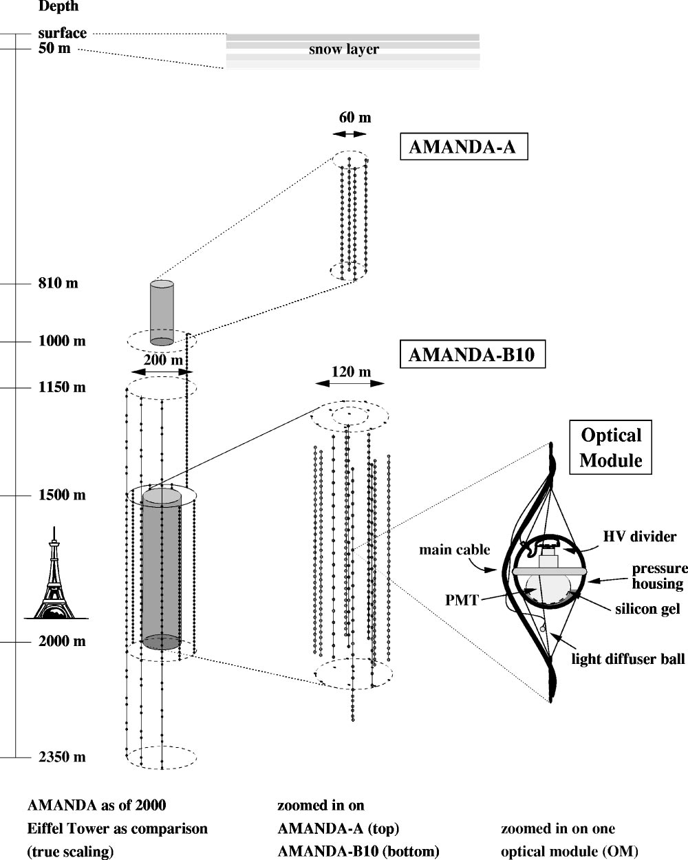
II. THE AMANDA DETECTOR
The AMANDA detector uses the 2.8 km thick ice sheet at
the South Pole as a neutrino target, Cherenkov medium and
cosmic ray flux attenuator. The detector consists of vertical
strings of optical modules
~
OMs
!
—photomultiplier tubes
sealed in glass pressure vessels—frozen into the ice at depths
of 1500–2000 m below the surface. Figure 1 shows the cur
rent configuration of the AMANDA detector. The shallow
array, AMANDAA, was deployed at depths of 800 to 1000
m in 1993–1994 in an exploratory phase of the project. Stud
ies of the optical properties of the ice carried out with
AMANDAA showed a high concentration of air bubbles at
these depths, leading to strong scattering of light and making
accurate track reconstruction impossible. Therefore, a deeper
array of ten strings with 302 OMs was deployed in the aus
tral summers of 1995–1996 and 1996–1997 at depths of
1500–2000 m. This detector is referred to as AMANDA
B10, and is shown in the center of Fig. 1. The detector was
augmented by three additional strings in 1997–1998 and six
in 1999–2000, forming the AMANDAII array.
In AMANDA B10, an optical module consists of a single
8 in. Hamamatsu R59122 photomultiplier tube
~
PMT
!
housed in a glass pressure vessel. The PMT is optically
coupled to the glass housing by a transparent gel. Each mod
ule is connected to electronics on the surface by a dedicated
electrical cable, which supplies high voltage and carries the
anode signal of the PMT. For each event, the optical module
is read out by a peaksensing ADC and a TDC capable of
registering up to eight separate pulses. The overall precision
of measurement of photon arrival times is approximately
5 ns. Details of deployment, electronics and data acquisition,
calibration, and the measurements of geometry, timing reso
lution, and the optical properties of the ice can be found in
@
1,2
#
.
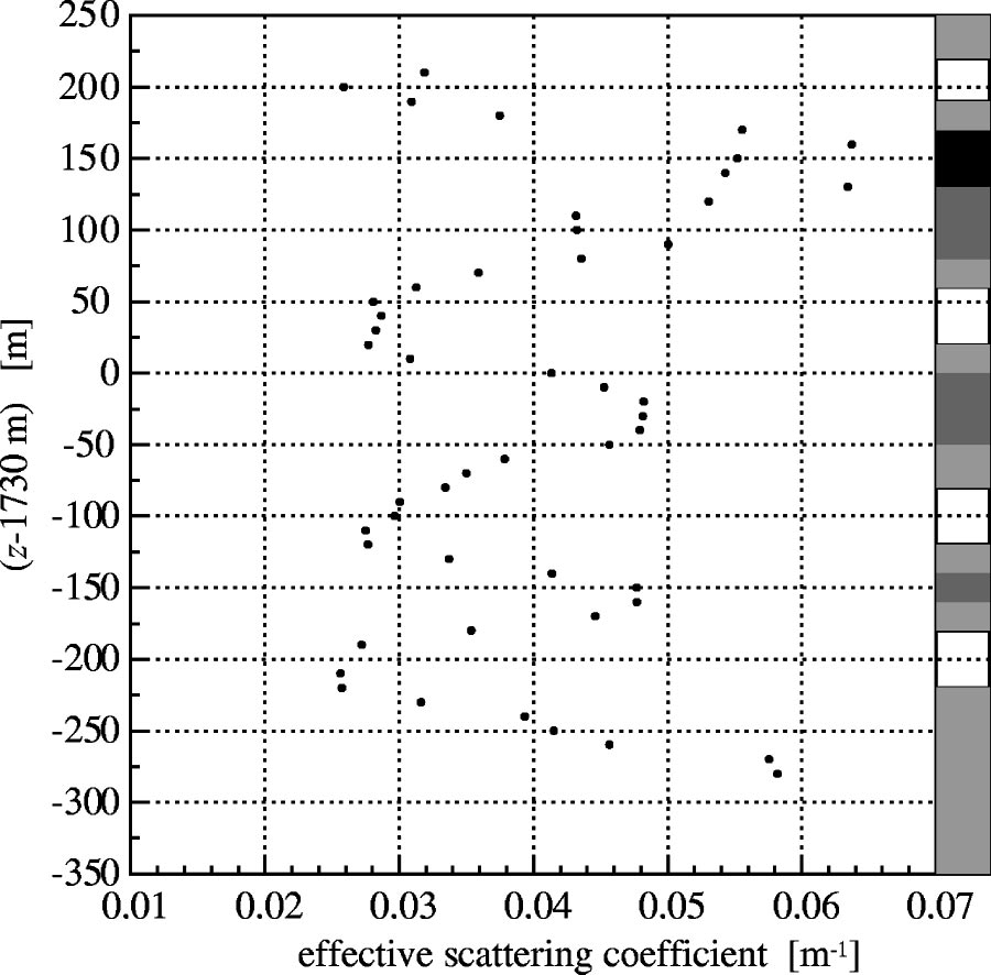
The optical properties of the polar ice in which
AMANDA is embedded have been studied in detail, using
both light emitters located on the strings and the downgoing
muon flux itself. These studies
@
3
#
have shown that the ice is
not perfectly homogeneous, but rather that it can be divided
into several horizontal layers which were laid down by vary
ing climatological conditions in the past
@
4
#
. Different con
centrations of dust in these layers lead to a modulation of the
FIG. 1. The present AMANDA detector. This paper describes
data taken with the ten inner strings shown in expanded view in the
bottom center.
J. AHRENS
et al.
PHYSICAL REVIEW D
66
, 012005
~
2002
!
0120052
scattering and absorption lengths of light in the ice, as shown
in Fig. 2. The average absorption length is about 110 m at a
wavelength of 400 nm at the depth of the AMANDAB10
array, and the average effective scattering length is approxi
mately 20 m.
III. DATA AND SIMULATION
The data analyzed in this paper were recorded during the
austral winter of 1997, from April to November. Subtracting
downtime for detector maintenance, removing runs in which
the detector behaved abnormally and correcting for deadtime
in the data acquisition system, the effective livetime was
130.1 days.
Triggering was done via a majority logic system, which
demanded that 16 or more OMs report signals within a slid
ing window of 2
m
s. When this condition was met, a trigger
veto was imposed and the entire array read out. The raw
trigger rate of the array was on average 75 Hz, producing a
total data set of 1.05
3
10
9
events.
Random noise was observed at a rate of 300 Hz for OMs
on the inner four strings and 1.5 kHz for tubes on the outer
six, the difference being due to different levels of concentra
tion of radioactive potassium in the pressure vessels
~
details
on noise rates can be found in Ref.
@
5
#!
. A typical event has
a duration of 4.5
m
s, including the muon transit time and the
light diffusion times, so random noise contributed on average
one PMT signal per event.
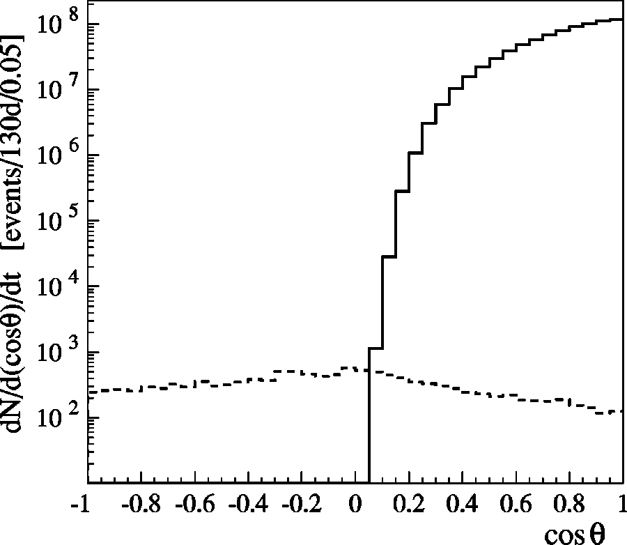
Almost all of the events recorded were produced by
downgoing muons originating in cosmic ray showers. Trig
gers from atmospheric neutrinos contribute only a few tens
of events per day, a rate small compared to the event rate
from cosmic ray muons, as shown in Fig. 3. The main task of
AMANDA data analysis is to separate these neutrino events
from the background of cosmicray muons. Monte Carlo
~
MC
!
simulations of the detector response to muons pro
duced by neutrinos or by cosmic rays were undertaken to
develop techniques of background rejection.
Downgoing muons were generated by atmospheric
shower simulations of isotropic protons with
BASIEV
@
6
#
or
protons and heavier nuclei with
CORSIKA using the QGSJET
generator
@
7,8
#
, and tracked to the detector with the muon
propagation code
MUDEDX
@
9,10
#
. Two other muon propaga
tion codes were used to check for systematic differences:
PROPMU
@
11
#
with a 30% lower rate and
MMC
@
12
#
with a
slightly higher rate. A total of 0.9
3
10
8
events were simu
lated. Most characteristics of the events generated with
BASIEV
were found to be similar to the more accurate
CORSIKAbased simulation. For the latter, the primary cosmic
ray flux as described by WiebelSooth and Biermann
@
13
#
was used. The curvature of the Earth has been implemented
in
CORSIKA to correctly describe the muon flux at large ze
nith angles. The event rate based on this Monte Carlo was 75
Hz and compares reasonably well with the observed rate of
100 Hz
~
after deadtime correction
!
. The detector response to
muons was modeled by calculating the photon fields pro
duced by continuous and stochastic muonic energy losses
@
14
#
, and simulating the response of the hardware to these
photons
@
15,16
#
. Upgoing muons were generated by a propa
gation of atmospheric neutrinos, which were tracked through
the Earth and allowed to interact in the ice in or around the
detector or in the bedrock below
@
17,18
#
. Muons that were
generated in the bedrock were propagated using
PROPMU
@
11
#
until they reached the rockice boundary at the depth of 2800
m. The muons were then propagated through the ice in the
same way as those from cosmic ray showers. The atmo
spheric neutrino flux was taken from Lipari
@
19
#
.
The Cherenkov photon propagation through the ice was
modeled to create multidimensional tables of density and
FIG. 2. Variation of the optical properties with depth. The effec
tive scattering coefficient at a wavelength of 532 nm is shown as a
function of depth. The
z
axis is pointing upwards and denotes the
vertical distance from the origin of the detector coordinate system
located at a depth of 1730 m. The shaded areas on the side indicate
layers of constant scattering coefficient as used in the Monte Carlo
simulation.
FIG. 3. The zenith angle distribution of simulated AMANDA
triggers per 130.1 days of lifetime. The solid line represents triggers
from downgoing cosmic ray muons generated by
CORSIKA. The
dashed line shows triggers produced by atmospheric neutrinos.
OBSERVATION OF HIGH ENERGY ATMOSPHERIC... PHYSICAL REVIEW D
66
, 012005
~
2002
!
0120053
arrival time probability distributions of the photon flux.
These photon fields were calculated for pure muon tracks
and for cascades of charged particles. A real muon track was
modeled as a superposition of the photon fields of a pure
muon track and the stochastic energy losses based on cas
cades. The photon fields were calculated out to 400 m from
the emission point, taking into account the orientation of the
OM with respect to the muon or cascade. In the detector
simulation, the ice was modeled as 16 discrete layers, as
indicated by the shaded areas in Fig. 2. The spectral proper
ties of the photomultiplier sensitivity, the glass, the gel, and,
most importantly, the ice itself were included in the simula
tion of the photon propagation. The probability of photon
detection depends on the Fresnel reflectance at all interfaces,
transmittances of various parts, and quantum and collection
efficiencies of the PMT. The relevant physical parameters
have been measured in the laboratory, so that the spectral
sensitivity of the OM could be evaluated. Two types of OMs,
differing in the type of pressure vessel, were used in the
construction of AMANDAB10. The inner four strings
~
AMANDAB4
!
use Billings housings while the outer six
strings use Benthos housings.
~
Benthos Inc. and Billings In
dustries are the manufacturers of the glass pressure vessels.
Benthos and Billings are registered trademarks of the respec
tive companies.
!
The two types of housing have different
optical properties. The Benthos OMs have an effective quan
tum efficiency of 21% at a wavelength of 395 nm for plane
wave photons incident normal to the PMT photocathode.
Ninety percent of the detected photons are in the spectral
range of 345–560 nm.
An additional sensitivity effect arises from the ice sur
rounding the OMs. The deployment of OMs requires melting
and refreezing of columns of ice, called ‘‘hole ice’’ hereafter.
This cycle results in the formation of bubbles in the vicinity
of the modules, which increase scattering and affects the
sensitivity of the optical modules in ways that are not under
stood in detail. Since the total volume of hole ice is small
compared to bulk ice in the detector
~
columns of 60 cm di
ameter, compared to 30 m spacing between strings
!
, its effect
on optical properties can be treated as a correction to the OM
angular sensitivity. The increased scattering of photons in the
hole ice has been simulated and compared to data taken with
laser measurements
in situ
to assess the magnitude of this
effect. This comparison provides an OM sensitivity correc
tion that reduces the relative efficiency in the forward direc
tion, but enhances it in the sideways and backward direc
tions. The sensitivity in the backward hemisphere
(90° –180°) relative to the sensitivity integrated over all
angles (0° –180°) of the optical sensor increases from 20%
to 27%, due to this correction, while the average relative
sensitivity in the forward direction (0° –90°) drops from
80% to 73%. In other words, an OM becomes a somewhat
more isotropic sensor.
The effective angular sensitivity of the OMs was also as
sessed using the flux of downgoing atmospheric muons as a
test beam illuminating both the 295 downward facing OMs
and the 7 upward facing OMs. We assumed that the response
of the upward facing OMs to light from downward muons is
equivalent to the response of the downward facing OMs to
light from upward moving muons. Based on this assumption
we derived a modified angular response function
~
later re
ferred to as
ANGSENS
!
, which resulted in a effective reduc
tion of the absolute OM sensitivity in forward direction. In
this model the effective relative sensitivity is 67% in the
forward hemisphere, and 33% in the backward hemisphere.
This correction will be used to estimate the effect of system
atic uncertainties in the angular response on the final neu
trino analysis.
The simulation of the hardware response included the
modeling of gains and thresholds and random noise at the
levels measured for each OM. The transit times of the cables
and the shapes of the photomultiplier pulses, ranging from
170 to 360 ns full width at half maximum
~
FWHM
!
, were
included in the trigger simulation. Multiphoton pulses were
simulated as superimposed single photoelectron waveforms.
In all, some 8
3
10
5
seconds of cosmic rays were simulated,
corresponding to 7% of the events contained in the 1997 data
set.
IV. EVENT RECONSTRUCTION
The reconstruction of muon events in AMANDA is done
offline, in several stages. First, the data are ‘‘cleaned’’ by
removing unstable PMTs and spurious PMT signals
~
or
‘‘hits’’
!
due to electronic or PMT noise. The cleaned events
are then passed through a fast filtering algorithm, which re
duces the background of downgoing muons by one order of
magnitude. This reduction allows the application of more
sophisticated reconstruction algorithms to the remaining data
set.
Because of the complexity of the task, and in order to
increase the robustness of the results, two separate analyses
of the 1997 data set were undertaken. Both proceeded along
the general lines described above, but differ in the details of
implementation. The preliminary stages, which are very
similar in both analyses, are described here. The particulars
of each analysis will be described in Secs. V and VI. A more
detailed description of the reconstruction procedure will be
published elsewhere
@
20
#
.
A. Cleaning and filtering
The first step in reconstructing events is to clean and cali
brate the data recorded by the detector. Unstable channels
~
OMs
!
are identified and removed on a runtorun basis. On
average, 260 of the 302 OMs deployed are used in the analy
ses. The recorded times of the hits are corrected for delays in
the cables leading from the OMs to the surface electronics
and for the amplitudedependent time required for a pulse to
cross the discriminator threshold. Hits are removed from the
event if they are identified as being due to instrumental
noise, either by their low amplitudes or short pulse lengths,
or because they are isolated in space by more than 80 m and
time by more than 500 ns from the other hits recorded in the
event. Pulses with short duration, measured as the time over
threshold
~
TOT
!
, are often related to electronic crosstalk in
the signal cables or the surface electronics. In analysis II,
TOT cuts are applied to individual channels beyond the stan
dard cleaning common to both analyses
~
see Sec. VI
!
.
J. AHRENS
et al.
PHYSICAL REVIEW D
66
, 012005
~
2002
!
0120054
Following the cleaning and the calibration, a ‘‘line fit’’ is
calculated for each event. This fit is a simple
x
2
minimiza
tion of the apparent photon flux direction, for which an ana
lytic solution can be calculated quickly
@
21
#~
see also
@
1
#!
.It
contains no details of Cherenkov radiation or propagation of
light in the ice. Hits arriving at time
t
i
at PMT
i
located at
r
i
W
are projected onto a line. The minimization of
x
2
5
(
i
(
r
W
i
2
r
W
0
2
v
W
lf
t
i
)
2
gives a solution for
r
W
0
and a velocity
v
W
lf
. The
results of this fit—at the first stage the direction
v
W
lf
/
u
v
W
lf
u
,at
later stages the absolute value of the velocity—are used to
filter the data set. Approximately 80–90 % of the data, for
which the line fit solution is steeply downgoing, are rejected
at this stage.
B. Maximum likelihood reconstruction
After the data have been passed through the fast filter,
tracks are reconstructed using a maximum likelihood
method. The observed photon arrival times do not follow a
simple Gaussian distribution attributable to electronic jitter;
instead, a tail of delayed photons is observed. The photons
can be delayed predominantly by scattering in the ice that
causes them to travel on paths longer than the length of the
straight line inclined at the Cherenkov angle to the track.
Also, photons emitted by scattered secondary electrons gen
erated along the track will have emission angles other than
the muon Cherenkov angle. These effects generate a distri
bution of arrival times with a long tail of delayed photons.
We construct a probability distribution function describ
ing the expected distribution of arrival times, and calculate
the likelihood
L
time
of a given reconstruction hypothesis as
the product of the probabilities of the observed arrival times
in each hit OM:
L
time
5
)
i
5
1
N
hit
p
~
t
res
(
i
)
u
d
’
(
i
)
,
u
ori
(
i
)
!
~
1
!
where
t
res
5
t
obs
2
t
Cher
is the time residual
~
the delay of the
observed hit time relative to that expected for unscattered
propagation of Cherenkov photons emitted by the muon
!
,
and
d
’
and
u
ori
are the distance of the OM from the track and
the orientation of the module with respect to the track. The
probability distribution function
p
includes the effects of
scattering and absorption in the bulk ice and in the refrozen
ice around the modules. The functional form of
p
is based on
a solution to a transport equation of the photon flux from a
monochromatic point source in a scattering medium
@
22,23
#
.
The free parameters of this function are then fit to the ex
pected time profiles that are obtained by a simulation of the
photon propagation from muons in the ice
@
14,22
#
. Varying
the track parameters of the reconstruction hypothesis, we
find the maximum of the likelihood function, corresponding
to the best track fit for the event. The result of the fit is
described by five parameters: three (
x
,
y
,
z
) to determine a
reference point, and two (
u
,
f
) for the zenith and azimuth of
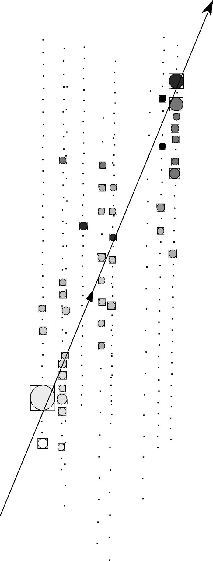
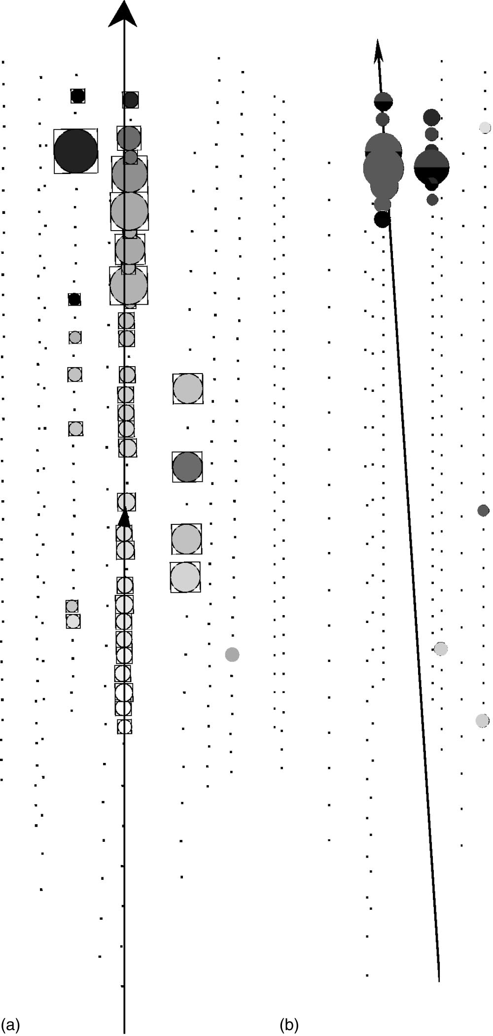
the track direction. Figure 4 shows an event display of two
upgoing muon events together with the reconstructed tracks.
C. Quality parameters
The set of apparently upgoing tracks provided by the re
construction procedure exceeds the expected number of up
going tracks from atmospheric neutrino interactions by one
to three orders of magnitude, depending on the details of the
reconstruction algorithm
~
see Secs. V and VI
!
. In order to
reject the large number of ‘‘fake events’’—events generated
by a downgoing muon or cascade, but seemingly having an
upgoing structure—we impose additional requirements on
the reconstructed events to obtain a relatively pure neutrino
sample. These requirements consist of cuts on observables
derived from the reconstruction and on topological event pa
rameters. Below, we describe the most relevant of the param
eters used.
FIG. 4. Event display of an upgoing muon event. The gray scale
indicates the flow of time, with early hits at the bottom and the
latest hits at the top of the array. The arrival times match the speed
of light. The sizes of the circles correspond to the measured ampli
tudes.
OBSERVATION OF HIGH ENERGY ATMOSPHERIC... PHYSICAL REVIEW D
66
, 012005
~
2002
!
0120055
1. Reduced likelihood, L
In analogy to a reduced
x
2
, we define a reduced likeli
hood
L
5
2
ln
L
time
N
hit
2
5
~
2
!
where
N
hit
2
5, the number of recorded hits in the event less
the five track fit parameters, is the number of degrees of
freedom. A smaller
L
corresponds to a higher quality of the
fit.
2. Number of direct hits, N
dir
The number of direct hits is defined as the number of hits
with time delays
t
res
smaller than a certain value. We use
time intervals of
@
2
15 ns,
1
25 ns
#
and
@
2
15 ns,
1
75 ns
#
, and denote the corresponding parameters as
N
dir
(25)
and
N
dir
(75)
, respectively. The negative extent of the window
allows for jitter in PMT rise times and for small errors in
geometry and calibration, while the positive side includes
these effects as well as delays due to scattering of the pho
tons. Events with many direct hits
~
i.e. , only slightly delayed
photons
!
are likely to be well reconstructed.
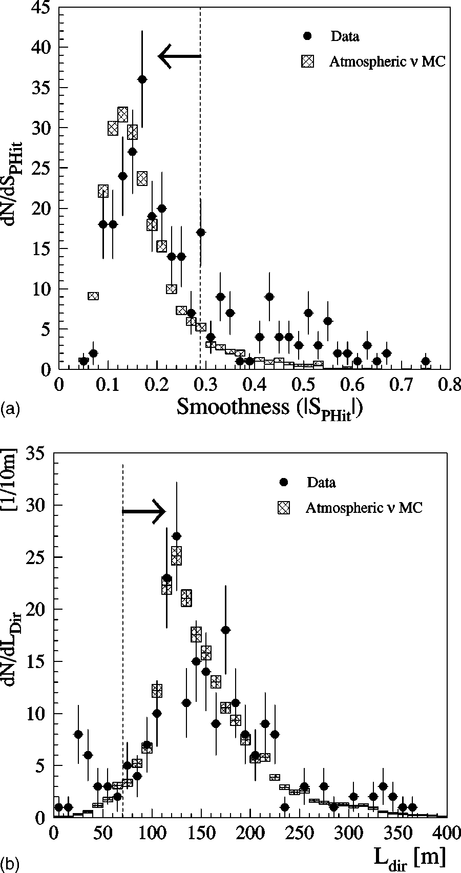
3. Track length, L
dir
The track length is defined by projecting each of the direct
hits onto the reconstructed track, and measuring the distance
between the first and the last hit. A cut on this parameter
rejects events with a small lever arm for the reconstruction.
Direct hits with time residuals of
@
2
15 ns,
1
75 ns
#
are
used for the measurement of the track length. Cuts on the
absolute length, as well as zenith angle dependent cuts
~
which take into account the cylindrical shape of the detec
tor
!
have been used. The requirement of a minimum track
length corresponds to imposing a muon energy threshold.
For example, a track length of 100 m translates into a muon
energy threshold of about 25 GeV.
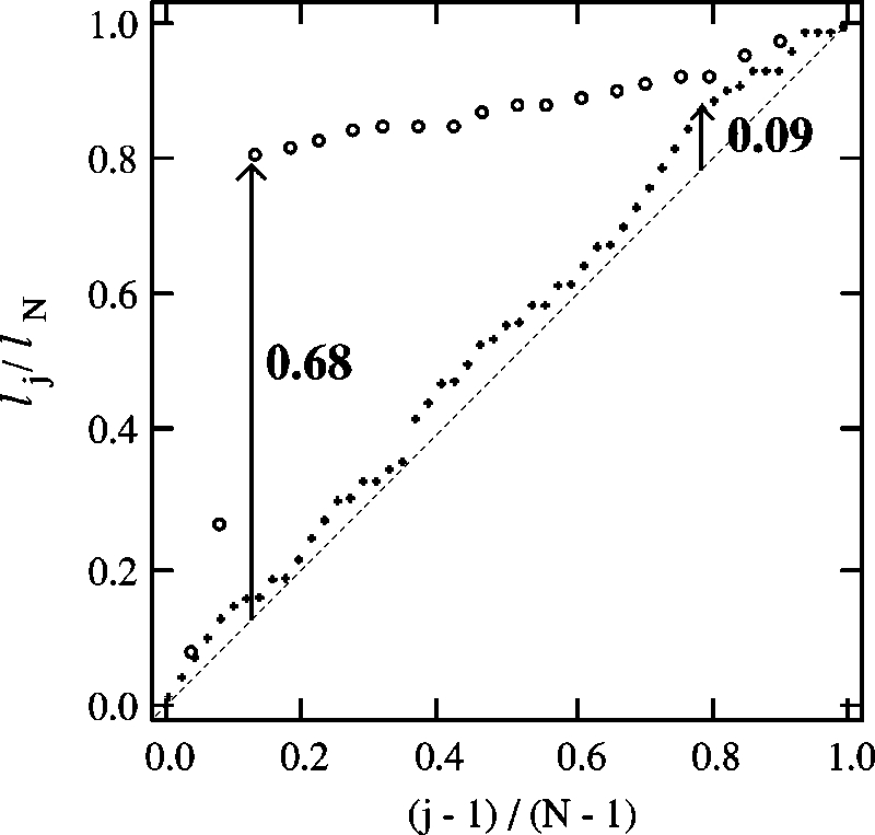
4. Smoothness, S
The ‘‘smoothness’’ parameter is a check on the self
consistency of the fitted track. It measures the constancy of
light output along the track. Highly variable apparent emis
sion of light usually indicates that the track either has been
completely misreconstructed or that an underlaying muonic
Cherenkov light was obscured by a very bright stochastic
light emission, which usually leads to poor reconstruction.
The smoothness parameter was inspired by the Kolmogorov
Smirnov test of the consistency of two distributions; in our
case the consistency of the observed hit pattern with the hy
pothesis of constant light emission by a muon.
Figure 5 shows two events to illustrate the characteristics
of the smoothness parameter. One event is a long uniform
track, which was well reconstructed. The other event is a
background event which displays a very poor smoothness.
The simplest definition of the smoothness is given by
S
5
max
~
u
S
j
u
!
, where
S
j
5
j
2
1
N
2
1
2
l
j
l
N
.
~
3
!
Figure 6 illustrates the smoothness parameter for the two
events displayed in Fig. 5. Here
l
j
is the distance along the
track between the points of closest approach of the track to
the first and the
j
th
hit modules, with the hits taken in order
of their projected position on the track.
N
is the total number
FIG. 5. Two muon events: The upgoing muon event shown on
the left has a smooth distribution of hits along the track. The track
like hit topology of this event can be used to distinguish it from
background events. The event on the right is a background event
with a poor smoothness value.
J. AHRENS
et al.
PHYSICAL REVIEW D
66
, 012005
~
2002
!
0120056
of hits. Tracks with hits clustered at the beginning or end of
the track have
S
j
approaching
1
1or
2
1, leading to
S
5
1.
High quality tracks such as the event on the left side of Fig.
5, with
S
close to zero, have hits equally spaced along the
track.
5. Sphericity
Treating the hit modules as point masses, we can form a
tensor of inertia for each event, describing the spatial distri
bution of the hits. Diagonalizing the tensor of inertia yields
as eigenvalues
I
i
the moments of inertia about the principal
axes of rotation. For a long, cylindrical distribution of hit
modules, two moments will be much larger than the third.
We can reject spherical events, such as those produced by
muon bremsstrahlung, by requiring that the normalized mag
nitude of the smallest moment,
I
1
/
(
I
i
, be small.
D. Principal methods of the analyses
The two analyses of the data diverge after the filtering
stage, following different approaches to event reconstruction
and background rejection.
Analysis I uses an improved likelihood function based on
a more detailed description of the photon response
@
22
#
, fol
lowed by a set of stepwise tightened cuts. Analysis II uses a
Bayesian reconstruction
@
24
#
in which the likelihood is mul
tiplied by a zenith angle dependent prior function, resulting
in a strong rejection of downgoing background.
Rare backgrounds due to unsimulated instrumental ef
fects, such as crosstalk between signal channels and un
stable voltage supply, were identified in the course of the
analyses. These effects either produced spurious triggers, or,
more often, spurious hits that caused the event to be misre
constructed. Different but comparably efficient techniques
were developed to treat these backgrounds. In analysis I the
event topology is inspected; if the spatial pattern of hit OMs
is inconsistent with the reconstructed muon trajectory, the
event is rejected. Analysis II attempts to remove the anoma
lous hits or triggers through identification of characteristic
correlations in signal amplitudes and times, which consider
ably reduces the rate of these misreconstructions.
At this stage the data set in each analysis is reduced to
several thousand events out of the original 1.05
3
10
9
, but the
data are still background dominated. The prediction for at
mospheric neutrinos is about 500 at this point.
For the final selection of a nearly pure sample of neutrino
induced events, cuts on characteristic observables are tight
ened until the remaining background disappears. The two
analyses use different techniques to choose their final cuts,
but obtain comparable efficiencies. Further details of the
analyses can be found in Refs.
@
25–27
#
.
V. ANALYSIS I
In this analysis the data were processed through three lev
els of initial cuts, designed to reduce the number of back
ground events to a manageable size for the final cut evalua
tion. After a first filtering based on the line fit
~
level 1
!
, cuts
on the zenith angle, the number of direct photons, and the
likelihood of the fitted track obtained by the maximum like
lihood reconstruction were applied
~
level 2
!
.
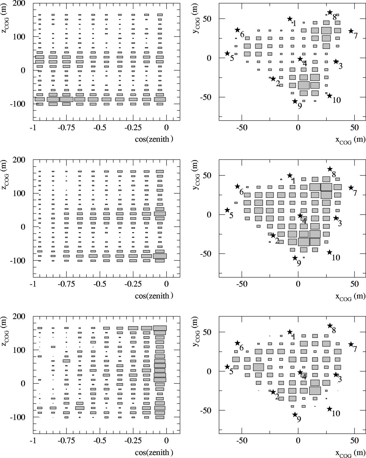
A. Removal of cascadelike events and detector artifacts
A third filter level used the results of an iterative likeli
hood reconstruction with varying track initializations, a fit
based on the hit probabilities
@
see Eq.
~
4
!#
and a reconstruc
tion to the hypothesis of a high energy cascade, e.g., due to a
bright seconday muon bremsstrahlung interaction.
The first two levels of filtering consisted of relatively
weak cuts on basic parameters like the zenith angle and like
lihood. They reduced the data set to about 4
3
10
5
events. At
this stage, residual unsimulated instrumental features become
apparent, e.g., comparatively high amplitude crosstalk pro
duced when a downgoing muon emits a bright shower in the
center of the detector. Such events are predominantly recon
structed as moving vertically upward and can be identified in
the distribution of the center of gravity
~
COG
!
of hits. Its
vertical component (
z
COG
) shows unpredicted peaks in the
middle and the bottom of the detector
@
see also Fig. 14
~
top
!
,
demonstrating the effect for analysis II
#
, while the horizontal
components (
x
COG
and
y
COG
) show an enhancement of hits
towards the outer strings. These strings are read out via
twisted pair cables, as opposed to the coaxial cables used on
the inner strings. The twisted pair cables were found to be
more susceptible to crosstalk signals. Note that variations in
the optical parameters of the ice due to past climatological
episodes also produce some vertical structure.
We developed additional COG cuts on the topology of the
events in order to remove these backgrounds. These cuts,
which depend on the reconstructed zenith angle, use the
track lengths
L
dir
and the normalized smallest eigenvalues of
the tensor of inertia (
I
1
/
(
I
i
).
FIG. 6. Illustration of the smoothness parameter, which com
pares the observed distribution of hits to that predicted for a muon
emitting Cherenkov light. In the simplest formulation, shown here,
the prediction is given as a straight line. A large deviation from a
straight line
~
0. 68
!
is found for the event on the right in Fig. 5. The
high quality tracklike event on the left in Fig. 5 displays a small
deviation
~
0.09
!
.
OBSERVATION OF HIGH ENERGY ATMOSPHERIC... PHYSICAL REVIEW D
66
, 012005
~
2002
!
0120057
Figure 7 shows the different components of the center of
gravity of the hits and the reconstructed zenith angle before
and after application of the COG cuts, and the Monte Carlo
prediction for fake upward events stemming from misrecon
structed downgoing muons. The cuts remove most of the
unsimulated background—in particular that far from the
horizon—and bring experiment and simulation into much
better agreement.
In order to verify the signal passing rates, these cuts and
those from the previous levels were applied to a subsample
of unfiltered
~
i.e., downgoing
!
events but with the zenith
angle dependence of the cuts reversed, thus using the abun
dant cosmic ray muons as standins for upgoing muons.
In all, these three levels of filtering reduced the data set by
a factor of approximately 10
5
~
see Table II
!
.
B. Multiphotoelectron likelihood and hit likelihood
Before the final cut optimization the last, most elaborate
reconstruction was applied, combining the likelihoods for the
arrival time of the first of muliple photons in a PMT with the
likelihoods for PMTs to have been hit or have not been hit.
The probability densities
p
(
t
res
(
i
)
u
d
’
(
i
)
,
u
ori
(
i
)
)
@
see Eq.
~
1
!
,
Sec. IV B
#
describe only the arrival times of single photons.
Density functions for the multiphotoelectron case have to
include the effect of repeatedly sampling the distribution of
photon arrival times. For several detected photons, the first
of them is usually less scattered than the average photon
~
which defines the single photoelectron case
!
. Therefore the
leading edge of a PMT pulse composed of multiple photo
electrons
~
MPE
!
will be systematically shifted to earlier
times compared to a single photoelectron. The
MPE likeli
hood
L
time
MPE
@
22
#
uses the recorded amplitude information to
model this shift.
In the reconstructions mentioned so far, the timing infor
mation from hit PMTs was used. However, a PMT which
was
not
hit also delivers information. The
hit likelihood
L
hit
does not depend on the arrival times but represents the prob
ability that the track produced the observed hit pattern. It is
constructed from the probability densities
p
hit
(
d
’
(
i
)
,
u
ori
(
i
)
) that
a given PMT
i
was hit if it was in fact hit, and the probabili
ties
@
1
2
p
hit
(
d
’
(
j
)
,
u
ori
(
j
)
)
#
that a given PMT
j
was not hit if it
was not hit:
L
hit
5
)
i
5
1
N
hit
p
hit
~
d
’
(
i
)
,
u
ori
(
i
)
!
)
i
5
N
hit
1
1
N
OM
~
1
2
p
hit
~
d
’
(
i
)
,
u
ori
(
i
)
!!
~
4
!
where the first product runs over all hit PMTs and the second
over all nonhit PMTs.
The likelihood combining these two probabilities is
FIG. 7. Characteristic distributions of the cen
ter of gravity
~
COG
!
of events. The figures on the
left show the distribution of the depth
z
COG
ver
sus the reconstructed zenith angle. The figures on
the right show the horizontal location of events in
the
x
COG
y
COG
plane of events with 0 m
,
z
COG
,
50 m. The positions of the strings are marked
by stars. Top: Experimental data before applica
tion of the COG cuts. Middle: Experimental data
after application of the COG cuts. Bottom: Ex
pectation from the BG simulation after cuts.
J. AHRENS
et al.
PHYSICAL REVIEW D
66
, 012005
~
2002
!
0120058
L
5
L
time
MPE
L
hit
.
~
5
!
A cut on the reconstructed zenith angle obtained from
fitting with
L
leaves less than 10
4
events in the data set,
defined as level 4 in Fig. 8.
C. Final separation of the neutrino sample
For the final stage of filtering, a method
~
CUTEVAL
!
was
developed to select and optimize the cuts taking into account
correlations between the cut parameters. A detailed descrip
tion of this method can be found in
@
27
#
. The principle of
CUTEVAL
is to numerically optimize the ratio of signal to
A
background by variation of the selection of cut parameters,
as well as the actual cut values. Parameters are used only if
they improve the efficiency of separation over optimized cuts
on all other already included parameters. A first optimization
was based purely on Monte Carlo simulations, with simu
lated atmospheric neutrinos for signal and simulated down
going muons forming the background. This optimization
yielded four such independent parameters. Two other optimi
zations involved experimental data. In both cases, experi
mental data have been defined as the background sample. In
one case, the signal was represented by atmospheric neutrino
Monte Carlo simulations, in the other by experimental data
subjected to zenith angle inverted cuts
~
i.e., to downward
events passing the quality cuts, but being ‘‘good’’ events
with respect to the upper hemisphere instead—like neutrino
candidates—with respect to the lower hemisphere
!
. These
latter optimizations yielded two additional parameters, which
rejected a small contribution of residual unsimulated back
grounds: coincident muons from simultaneous independent
air showers and events accompanied by instrumental artifacts
such as crosstalk. After application of these two cuts to
simulated and experimental data, the distributions of observ
ables agree to a satisfactory precision.
Once the minimal set of parameters is found, the optimal
cut values can be represented as a function of the number of
background events
N
BG
passing the cuts. The result is a path
through the cut parameter space which yields the best signal
efficiency for any desired purity of the signal, characterized
by
N
BG
. Using this representation, one can calculate the
number of events passing the cuts as a function of the fitted
N
BG
for signal and for background Monte Carlo program.
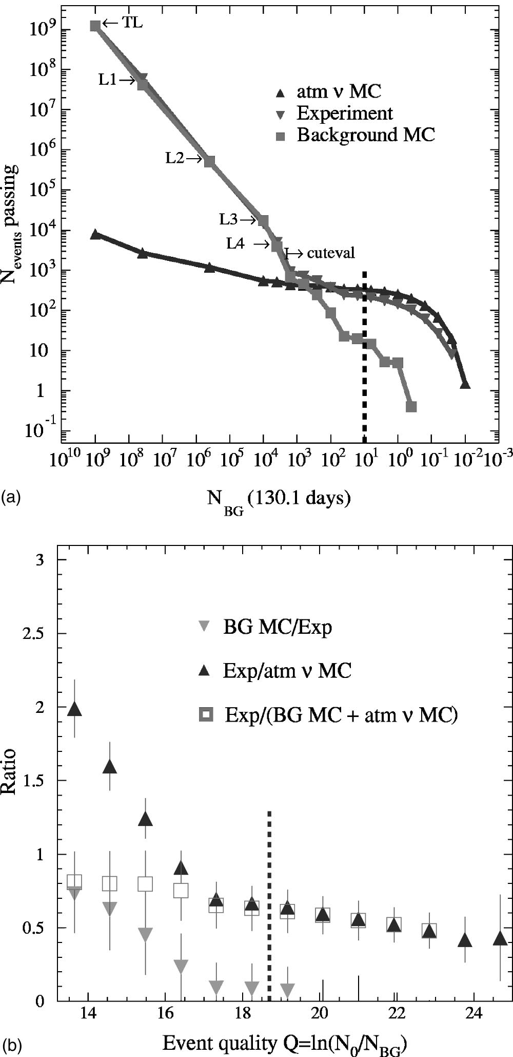
Figure 8
~
top
!
shows this dependence for simulations as well
as for experimental data, with
N
BG
varying from trigger level
to a level that leaves only a few events in the data set. One
observes that the actual background expectation falls roughly
linearly as the fitted
N
BG
is reduced. Below values of a few
hundred events the signal is expected to dominate the event
sample. The experimental curve follows the expectation from
the sum of background and signal Monte Carlo program. For
large
N
BG
, the observed event rate follows the background
expectation. At smaller
N
BG
, the experimental shape turns
over into the signal expectation and follows it nicely down to
the sample of events with highest quality
~
the smallest values
of
N
BG
!
. For a moderate background contamination of
N
BG
5
10, one gets a total of 223 neutrino candidates. The param
eters and cut values as obtained by the
CUTEVAL procedure
are summarized in Table I.
Figure 8
~
bottom
!
translates the background parameter
N
BG
into an event quality parameter
Q
, defined as
Q
[
ln(
N
0
/
N
BG
)
5
ln(1.05
10
9
/
N
BG
). The plot shows the ratios
FIG. 8. The fitted background parameter
N
BG
. Top: Number of
events versus
N
BG
. Smaller values of
N
BG
correspond to harder
cuts. Below
N
BG
5
1500 the
CUTEVAL
parametrization was used to
calculate the cut values corresponding to
N
BG
. For larger values of
N
BG
the data points correspond to the cuts from the filter levels:
Level 4
~
see Sec. V B
!
, level 3, level 2, level 1, and trigger level
~
Table II
!
. Bottom: Ratios of events passing in the experimental
data compared to various Monte Carlo expectations for signal and
background as a function of event quality. The dashed line indicates
the final cuts.
OBSERVATION OF HIGH ENERGY ATMOSPHERIC... PHYSICAL REVIEW D
66
, 012005
~
2002
!
0120059
of events from the upper figure as a function of
Q
. At higher
qualities (
Q
.
17), the ratio of observed events to the atmo
spheric neutrino simulation flattens out with a further varia
tion of only 30%. The value at
Q
5
17 is approximately 0.6
for the standard Monte Carlo program
~
chosen in Fig. 8, top
!
and approximately unity for the
ANGSENS Monte Carlo pro
gram
~
chosen in Fig. 8, bottom
!
.
Table II lists the cut efficiencies for the atmospheric neu
trino simulation
~
with and without the implementation of the
angular sensitivity fitted model
ANGSENS
of the OMs—see
Secs. III and VII
!
, the background simulation of atmospheric
muons from air showers
~
without
ANGSENS
!
and the experi
mental data. Again, the experimental numbers agree well
with the background simulation up to the first two filter lev
els. Later, the Monte Carlo program underestimates the ex
perimental passing rates slightly. The last row shows the ex
pected numbers of events for the last stage of filtering. If, in
addition, the effect of neutrino oscillations
~
see Sec. VII
!
is
included, the atmospheric neutrino simulation including the
ANGSENS
model predicts 224 events, in closest agreement
with the experiment. However, the 5% effect due to oscilla
tions is smaller than our systematic uncertainty
~
see Sec.
VII
!
.
D. Characteristics of the neutrino candidates
1. Time distribution
Figure 9 shows the cumulative number of neutrino events
as well as the cumulative number of event triggers plotted
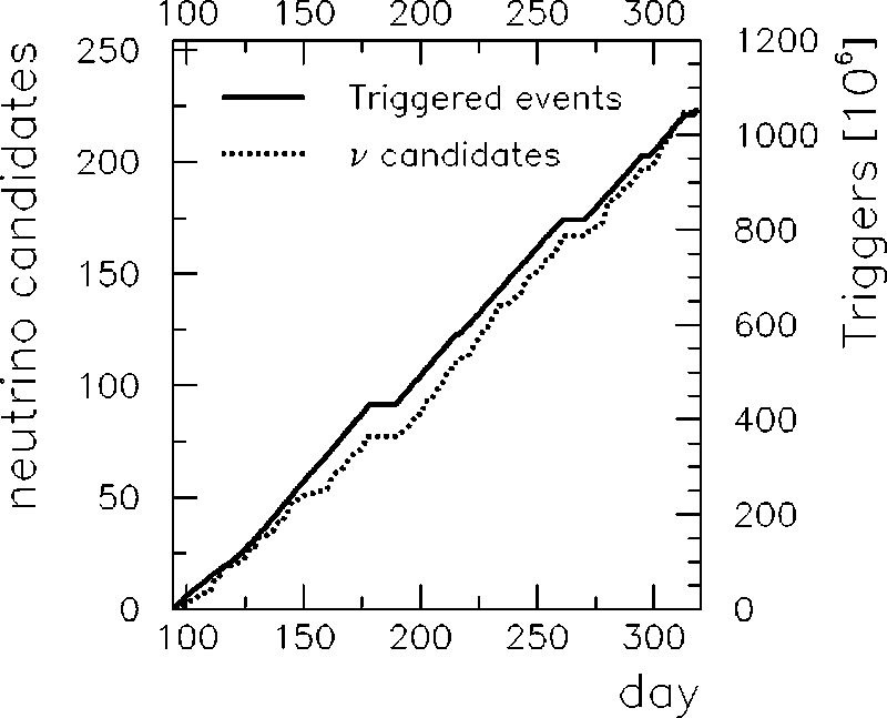
versus the day number in 1997. One can observe that the
neutrino events follow the number of triggers, albeit with a
small deficit during the Antarctic winter. This deficit is con
sistent with statistical fluctuations.
~
Actually, seasonal varia
tions slightly
de
crease the downward muon rate during the
Antarctic winter
@
28
#
and should result in a 10% deficit of
triggers with respect to upward neutrino events.
!
TABLE I. Final quality parameters and cuts obtained from the cut evaluation procedure. The ‘‘direct’’
time interval for variables
N
dir
,
L
dir
, and
S
dir
is
@
2
15 ns,
1
75 ns
#
. The first four rows show cut parameters
obtained by all
~
Monte Carlo and experimental
!
searches; the last two rows show two additional
~
weaker
!
cuts, which were found to remove unsimulated backgrounds.
Parameter Cut Explanation
u
S
u
,
0.28 See Sec. IV C 4
u
S
P
hit
u
/(
u
mpe
2
90°)
,
0.01 Tightens the requirement on the smoothness for
tracks
close to the horizon where background is high
(
N
dir
2
2)
L
dir
.
750 m Lever arm of the track times the number of
supporting points
log(
L
up
/
L
down
)
,2
7.7 Ratio of the likelihoods of the best
upgoing and best downgoing hypotheses
C
(mpe,lf)
,
35° Space angle between the results from the
multiphoton
likelihood reconstruction and the line fit. This cut
effectively removes crosstalk features.
A
(
S
dir
)
2
1
(
S
dir
P
hit
)
2
,
0.55 Parameter combining the two smoothness
definitions
~
here calculated using only direct hits
!
.
This cut effectively removes coincident muon
events from independent air showers.
TABLE II. The cut efficiencies for the atmospheric neutrino Monte Carlo
~
MC
!
prediction, the atmo
spheric muon background Monte Carlo prediction, and the experimental data for 130 days of detector
lifetime. Efficiencies are given for filter levels L1 to L4. L4 is the final selection. All errors are purely
statistical. The final background prediction of 7 events has been normalized at trigger level.
Filter level Atm.
n
Atm.
n
MC Atm.
m
MC Experimental
MC
ANGSENS
~
Background
!
data
Events at trigger level 8978 5759 9.03
3
10
8
1.05
3
10
9
Efficiency at level 1 0.34 0.37 0.4
3
10
2
1
0.5
3
10
2
1
Efficiency at level 2 0.15 0.15 0.4
3
10
2
3
0.4
3
10
2
3
Efficiency at level 3 0.7
3
10
2
1
0.7
3
10
2
1
0.7
3
10
2
5
0.1
3
10
2
4
Efficiency after final cuts 0.4
3
10
2
1
0.4
3
10
2
1
0.6
3
10
2
8
0.2
3
10
2
6
No. of events 362
6
4 237
6
67
6
5 223
passing final cuts normalized
J. AHRENS
et al.
PHYSICAL REVIEW D
66
, 012005
~
2002
!
01200510
2. Zenith angle distribution
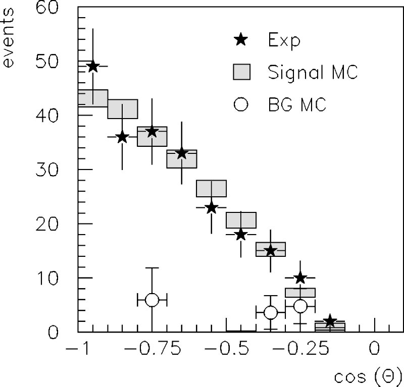
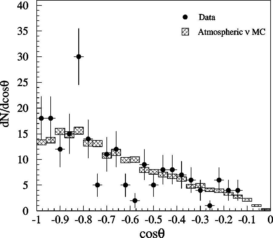
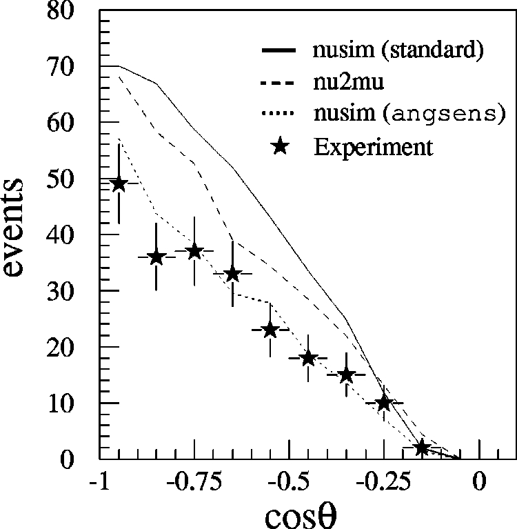
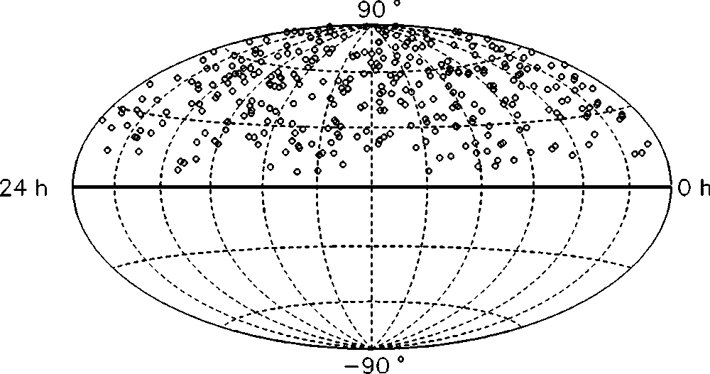
Figure 10 shows the zenith angle distribution of the 223
neutrino candidates compared to the Monte Carlo prediction
for atmospheric neutrinos
@
17
#
and the few remaining events
predicted by background simulations. Note that the Monte
Carlo prediction is normalized to experiment.
~
The total
number of events is 362 for the atmospheric neutrino simu
lation and 223 for experiment, i.e., there is a deficit of 39
percent in the absolute number of events.
!
There is good
agreement between the prediction and the experiment in the
shape of the angular distribution.
3. Characteristic distributions and visual inspection
Four methods were used to evaluate the effectiveness of
the analysis and the level of residual backgrounds:
~
a
!
N
2
1
cuts
,
~
b
!
unbiased variables
,
~
c
!
low level distributions
,
and
~
d
!
visual inspection
.
~
a
!
The
N
2
1
test
evaluates the
N
final cuts one by one
and yields an estimate of the background contamination in
the final sample. One applies all but one of the final cuts
~
the
one in the selected variable
!
, and plots the data in this vari
able. In the signal region of this variable
~
defined by the later
applied cut
!
shapes of experiment and signal Monte Carlo
program should agree. In the background region, the experi
mental data should approach the expected background shape.
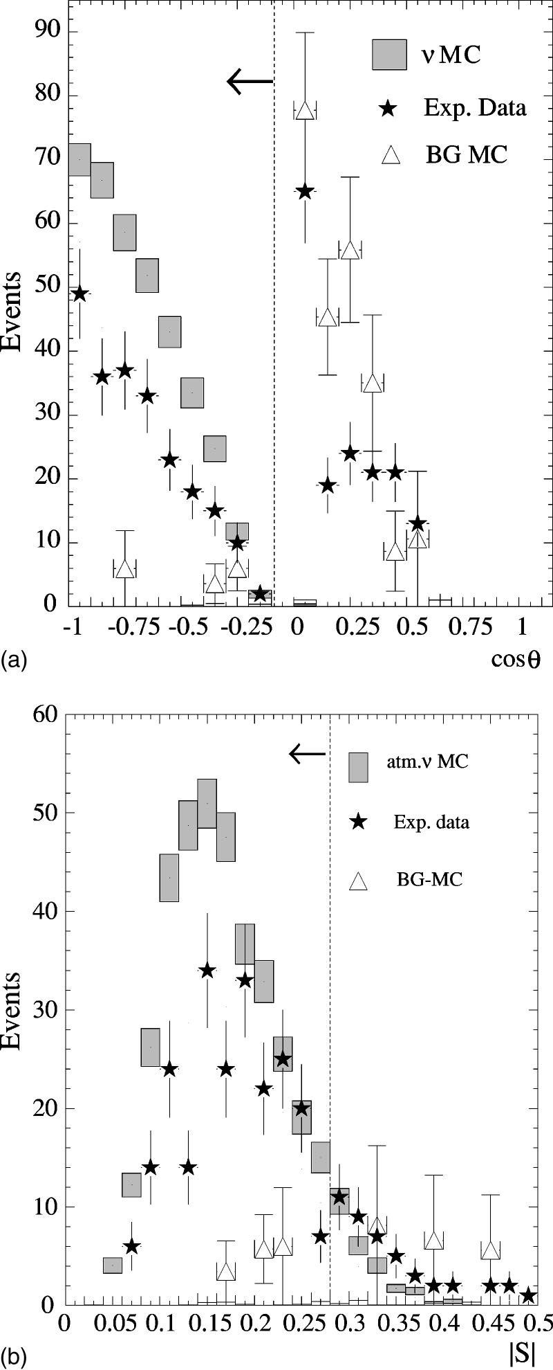
Figure 11 shows four of these distributions. The applied cut
is shown by a dotted line. All four cuts satisfy the test: the
shape of the distributions agree reasonably well on both sides
of the applied cuts. Two
N
2
1 distribution from analysis II
are shown in Fig. 19.
~
b
!
An obvious test is the investigation of distributions of
unbiased variables
~
i.e., variables to which no cuts have
been applied
!
in the final neutrino sample. Here, the experi
mental distributions follow the Monte Carlo signal expecta
tions nicely. Some deviations are observed, especially in the
number of OMs hit and the velocity
v
lf
obtained from the
line fit
~
see Sec. IV A
!
. However, as can be seen from Fig.
20, part of these disagreements disappear if the standard at
mospheric neutrino MC program is replaced by the
ANGSENS
MC version.
~
c
!
In order to account for possible pathological
low level
features in the data sample
~
especially crosstalk
!
,we
~
i
!
in
vestigated basic pulse amplitude and pulse width
~
TOT
!
dis
tributions and
~
ii
!
refitted all events after the crosstalk hit
cleaning procedure applied in analysis II
~
which is tighter
than the standard crosstalk cleaning introduced in Sec.
IV A
!
. Both these distributions and that for the recalculated
zenith angles show no significant deviation from the previ
ous ones. No crosstalk features are found in the resulting
neutrino sample.
~
d
!
Finally, a
visual inspection
of the full neutrino sample
was performed, by visually displaying each event like in Fig.
4. The visual inspection gives consistent results with the
other methods of background estimation and yields an upper
limit on the background contamination of muons from ran
dom coincident air showers
~
see below
!
.
E. Background estimation
The results of four independent methods of background
estimation are summarized in Table III.
First, the background Monte Carlo program itself gives an
estimate. It yields 7 events if rates are normalized to the
trigger level
~
see Table II
!
. Because the passing rates differ
slightly between the experiment
~
higher
!
and the background
Monte Carlo program
~
lower
!
, we made the conservative
choice to renormalize the background Monte Carlo program
to the level 3 experimental passing rate. This gives an esti
mate of about 16 background events in our final sample.
From the
N
2
1 distributions we obtained an alternative
approximation of the residual background. We renormalized
both signal and background MC events in the background
region to fit the number of experimental events in the back
ground region. The number of renormalized background
FIG. 9. The integrated exposure of the AMANDA detector in
1997. The figure shows the cumulative number of triggers
~
upper
curve
!
and the number of observed neutrino events
~
lower curve
!
versus the day number. The intervals with zero gradient correspond
to periods where the detector was not operating stably; data from
these periods were excluded from the analysis.
FIG. 10. Zenith angle distribution of the experimental data com
pared to simulated atmospheric neutrinos and a simulated back
ground of downgoing muons produced by cosmic rays. In this fig
ure the Monte Carlo prediction is normalized to the experimental
data. The error bars report only statistical errors.
OBSERVATION OF HIGH ENERGY ATMOSPHERIC... PHYSICAL REVIEW D
66
, 012005
~
2002
!
01200511
MC events in the signal region is then a background esti
mate. This estimate was performed
N
times
~
once for each
N
2
1 distribution
!
. The average over all
N
estimations yields
14 background events. Note that this averaging procedure is
reasonable only for the case of independent cuts. With the
method by which we have chosen the cut parameters, this
condition is satisfied to first approximation.
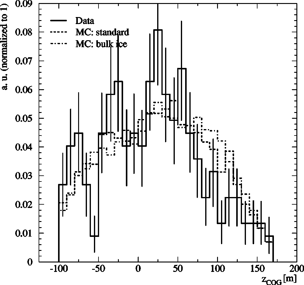
We have found that crosstalk hits are related to the char
acteristic triplepeak structure in the distribution of the ver
tical component of the center of gravity of hits (
z
COG
) which
has been discussed in Sec. V A—see Fig. 7 and also Fig. 14
~
top
!
. Since there are remaining cross talk hits which have
survived the standard cleaning
~
see Sec. IV A
!
, this distribu
tion was studied in detail. As shown in Fig. 12, the final
experimental sample of neutrino candidates shows no statis
tically significant excess with respect to the atmospheric neu
trino Monte Carlo prediction in the regions of the character
istic peaks. Therefore, an upper limit on this special class of
background was derived and yields
,
35 events.
The visual inspection of the neutrino sample yields 13
events. Seven of them show the signature of coincident
muons from independent air showers; i.e., two well separated
spatial concentrations of hits, each with a downward time
flow but with the lower group appearing earlier than the up
per one. Taking into account the scanning efficiencies which
were determined by scanning signal and background Monte
Carlo events, an upper limit of 23 events is obtained from
visual inspection.
Combining the results from the above methods, the ex
pected background is estimated to amount to 4 to 10% of the
223 experimental events.
FIG. 11. Two distributions of variables used as cut parameters in
the last filter level
~
see Table I for an explanation of the variables
!
.
In both cases, all final cuts with the exception of the variable plotted
have been applied. The cuts on the displayed parameters are indi
cated by the dashed vertical lines. Arrows indicate the accepted
parameter space.
FIG. 12. Distributions of
z
COG
for the experiment and atmo
spheric neutrino signal Monte Carlo program
MC standard
and
MC
bulk ice
denote two different ice models. The first includes vertical
ice layers in accordance with Fig. 2; the second uses homogeneous
ice.
TABLE III. Various estimates of the background remaining in
the experimental data sample of 223 neutrino candidates.
BG estimation method Estimation
BG MC 16
6
8
N
2
1 cuts 14
6
4
z
COG
distributions
,
35
Visual inspection
,
23
J. AHRENS
et al.
PHYSICAL REVIEW D
66
, 012005
~
2002
!
01200512
VI. ANALYSIS II
The second analysis follows a different approach; instead
of optimizing cuts to reject misreconstructed cosmic ray
muons, this analysis concentrates on improving the recon
struction algorithm with respect to background rejection. The
large downgoing muon flux implies that even a small frac
tion of downgoing muons misreconstructed as upgoing will
produce a very large background rate. Equivalently, for each
apparently upgoing event, there were many more downgoing
muons passing the detector than there were upgoing muons;
even though any single downgoing muon had only a small
probability of faking an upgoing event, the total probability
that the event was a fake is quite high.
A. Bayesian reconstruction
This analysis of the problem motivates a Bayesian ap
proach
@
24
#
to event reconstruction. Bayes’ theorem in prob
ability theory states that for two assertions
A
and
B
,
P
~
A
u
B
!
P
~
B
!
5
P
~
B
u
A
!
P
~
A
!
,
where
P
(
A
u
B
) is the probability of assertion
A
given that
B
is true. Identifying
A
with a particular muon track hypothesis
m
and
B
with the data recorded for an event in the detector,
we have
P
~
m
u
data
!
5
L
time
~
data
u
m
!
P
~
m
!
,
where we have dropped a normalization factor
P
(data)
which is a constant for the observed event. The function
L
time
is the regular likelihood function of Eq.
~
1
!
, and
P
(
m
)
is the socalled prior function, the probability of a muon
m
5
m
(
x
,
y
,
z
,
u
,
f
) passing through the detector.
For this analysis, we have used a simple onedimensional
prior function, containing the zenith angle information at
trigger level in Fig. 3. By accounting in the reconstruction
for the fact that the flux of downgoing muons from cosmic
rays is many orders of magnitude larger than that of upgoing
neutrinoinduced muons, the number of downgoing muons
that are misreconstructed as upgoing is greatly reduced. It
should be noted that the objections that are often raised with
respect to the use of Bayesian statistics in physics are not
relevant to this problem: the prior function is well defined
and normalized and independently known to relatively good
precision, consisting only of the fluxes of cosmic ray muons
and atmospheric muon neutrinos.
B. Removal of instrumental artifacts
The Bayesian reconstruction algorithm is highly efficient
at rejecting downgoing muon events. Of 2.6
3
10
8
events
passing the fast filter, only 5.8
3
10
4
are reconstructed as up
going. By contrast, the standard maximum likelihood recon
struction produces about 2.4
3
10
7
false upgoing reconstruc
tions. However, less than a thousand neutrino events are
predicted by Monte Carlo program, so it is clear that a sig
nificant number of misreconstructions remain.
Detailed inspection of the 5.8
3
10
4
events reveals that the
vast majority is produced by crosstalk overlaid on triggers
from downgoing muons emitting bright stochastic light near
the detector. This crosstalk confuses the reconstruction al
gorithm, producing apparently upgoing tracks. Because
crosstalk is not included in the detector simulation, the char
acteristics of the fakes are not predicted well by the simula
tion, and the rate of misreconstruction is much higher than
predicted.
The crosstalk is removed by additional hit cleaning rou
tines developed by examination of this crosstalk enriched
data set. For example, crosstalk in many channels can be
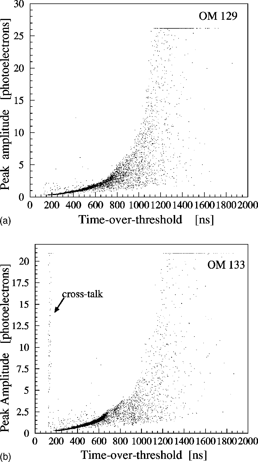
identified in scatter plots of pulse width vs amplitude, as
shown in Fig. 13. The pulse width is measured as time over
threshold
~
TOT
!
. Real hits form the distribution shown on
the left. High amplitude pulses should have large pulse
width. This is not the case for crosstalk induced pulses. In
channels with high levels of crosstalk, an additional vertical
FIG. 13. Pulse amplitude vs duration for modules on the outer
strings. Normal hits lie in the distribution shown in the upper figure.
High amplitude pulses of more than a few photoelectrons are valid
only if the pulse width is also large. Crosstalk induced pulses of
high amplitude are characterized by small time over threshold
~
TOT
!
. The cutoff seen at high amplitude is due to saturation of the
amplitude readout electronics.
OBSERVATION OF HIGH ENERGY ATMOSPHERIC... PHYSICAL REVIEW D
66
, 012005
~
2002
!
01200513
band is found at high amplitudes but short pulse widths, as
seen in the lower figure.
Other hit cleaning algorithms use the time correlation and
amplitude relationship between real and crosstalk pulses and
a map of channels susceptible to crosstalk and the channels
to which they are coupled. An additional instrumental effect,
believed to be caused by fluctuating high voltage levels, pro
duces triggers with signals from most OMs on the outer
strings but none on the inner four strings; some 500 of these
bogus triggers were also removed from the data set. The
5.8
3
10
4
upgoing events were again reconstructed after the
additional hit cleaning was applied. Only 4.9
3
10
3
~
8.4%
!
of
the events remained upgoing, compared to an expectation
from Monte Carlo program of 1855 atmospheric muon
events
~
37.8% of the total before the additional cleaning
!
,
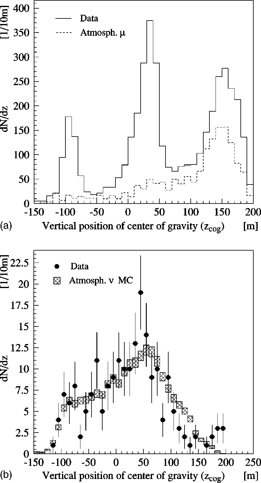
and 555 atmospheric neutrino events. Figure 14
~
top
!
shows
that while there has been a significant reduction in the instru
mental backgrounds, an unsimulated structure still remains
in the centerofgravity
~
COG
!
distribution for these remain
ing data events. The application of additional quality criteria
brings this distribution in agreement, as shown in Fig. 14
~
bottom
!
.
C. Quality cuts
The improvements in the reliability of the reconstruction
algorithm described above obviated the need for large num
bers of cut parameters or for careful optimization of the cuts.
Because the signaltonoise ratio of the upwardreconstructed
data is quite high to begin with, we have the possibility of
comparing the behavior of real and simulated data over a
wide range of cut strengths to verify that the data agree with
the predictions for upgoing neutrinoinduced muons, not
only in number but also in their characteristics. Using the cut
parameters described in Sec. IV C
~
with the likelihood re
placed by the Bayesian posterior probability
!
and a require
ment that events fitted as relatively horizontal by the line fit
filtering algorithm not be reconstructed as steeply upgoing
by the full reconstruction
~
a requirement that suppresses re
sidual crosstalk misreconstructions
!
, an index of event qual
ity was formed.
To do so, we rescale the six quality parameters described
above by the cumulative distributions of the simulated atmo
spheric neutrino signal, and consider the sixdimensional cut
space formed by the rescaled parameters. A point in this
space corresponds to fixed values of the quality parameters,
and events can be assigned to locations based on their track
length, sphericity, and so forth.
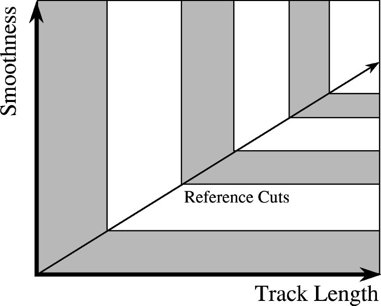
It is difficult to compare the distributions of data and
simulated up and downgoing muons directly because of the
high dimensionality of the space. We therefore project the
space down to a single— ‘‘quality’’ — dimension by divid
ing it into concentric rectangular shells, as illustrated in Fig.
15. The vertex of each shell lies on a line from the origin
through a reference set of cuts which are believed to isolate a
fairly pure set of neutrino events. Events in the full cut space
are assigned an overall quality value, based on the shell in
which they lie.
FIG. 14. Top: Event center of gravity distribution after recon
struction with special crosstalk cleaning algorithms applied to the
events. Unsimulated background remains. Bottom: The data agree
with the neutrino signal after application of additional quality cuts.
FIG. 15. Definition of event quality. Events are plotted in
N
dimensional cut space
~
two dimensions are shown here for clar
ity
!
. A line is drawn from the origin
~
no cuts
!
through a selected set
of cuts, and the space is divided into rectangular shells of equal
width. Events are assigned a quality
q
according to the shell in
which they are found.
J. AHRENS
et al.
PHYSICAL REVIEW D
66
, 012005
~
2002
!
01200514
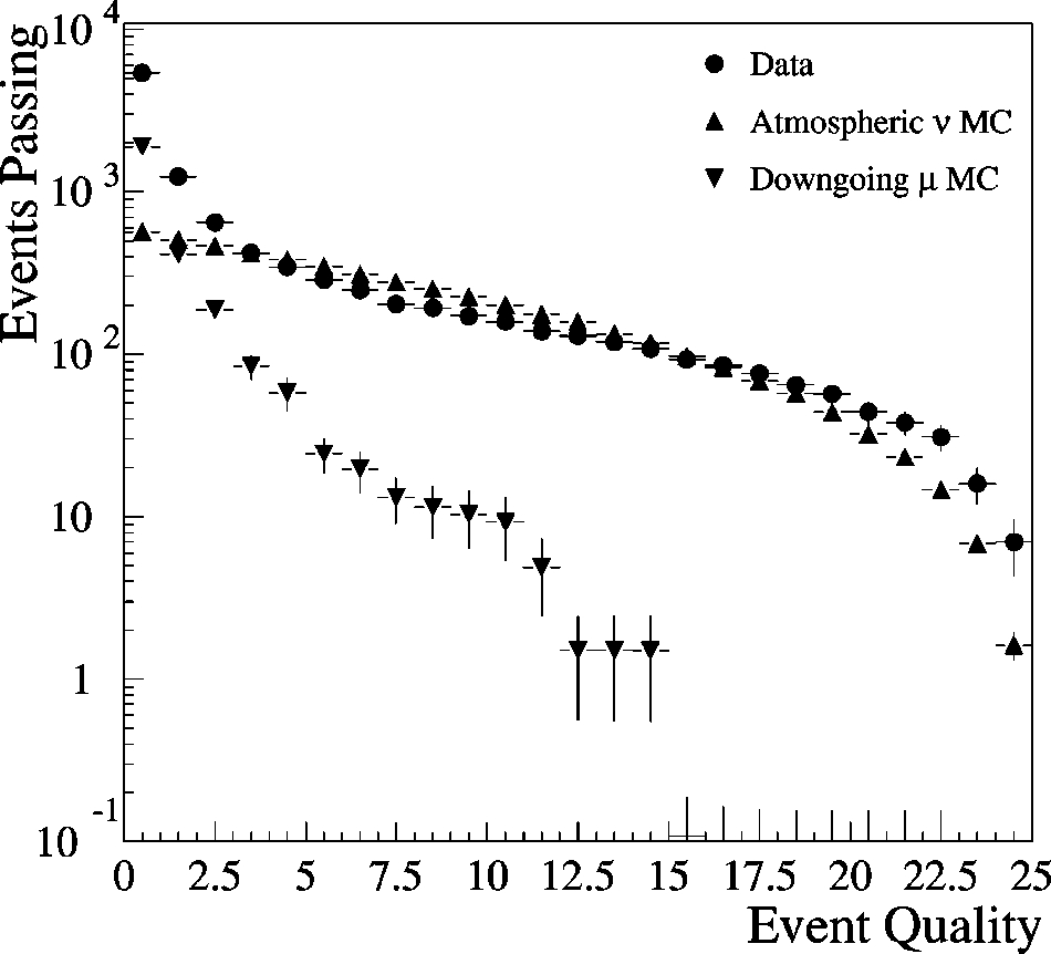
With this formulation we can compare the characteristics
of the data to simulated neutrino and cosmicray muon
events. Figure 16 compares the number of events passing
various levels of cuts; i.e., the integral number of events
above a given quality. At low qualities,
q
<
3, the data set is
dominated by misreconstructed downgoing muons, data as
well as the simulated background exceed the predicted neu
trino signal. At higher qualities, the passing rates of data
closely track the simulated neutrino events, and the predicted
background contamination is very low.
We can investigate the agreement between data and
Monte Carlo simulations more systematically by comparing
the differential number of events
within
individual shells,
rather than the total number of events passing various levels
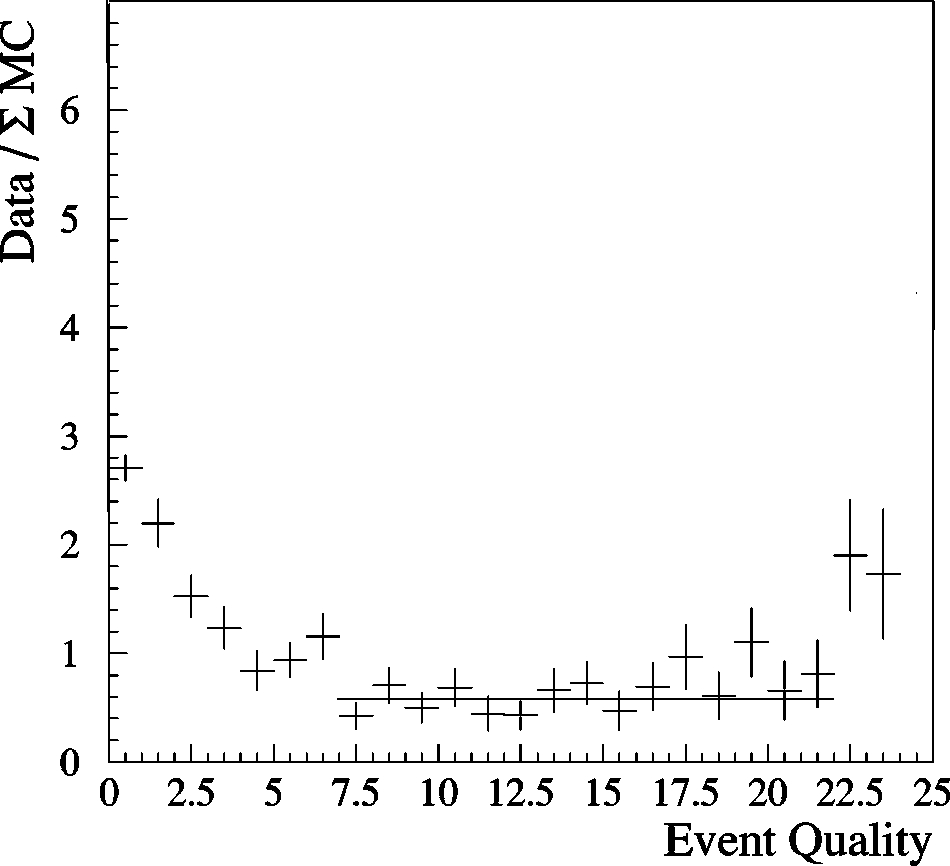
of cuts. This is done in Fig. 17, where the ratios of the
number of events observed to those predicted from the com
bined signal and background simulations are shown. One can
see that at low quality levels there is an excess in the number
of misreconstructed events observed. This is mainly due to
remaining crosstalk. There is also an excess, though statis
tically less significant, at very high quality levels, which is
believed to be caused by slight inaccuracies in the descrip
tion of the optical parameters of the ice. Nevertheless, over
the bulk of the range there is close agreement between the
data and the simulation, apart from an overall normalization
factor of 0.58. The absolute agreement is consistent with the
systematic uncertainties. It should be emphasized that the
quality parameter is a convolution of all six quality param
eters, and so the flat line in Fig. 17 demonstrates agreement
in the correlations between cut parameters.
D. Background estimation and signal description
If we reduce the 4917 upwardreconstructed events by
requiring a quality of at least 7 on the scale of Fig. 16, we
obtain a set of 204 neutrino candidates. The background con
tamination, which is due to misreconstructed downgoing
muons, was estimated in three ways. The first way is to
simulate the downgoing muon flux, bearing in mind that we
are looking at a very low tail (10
2
8
) of the total muon dis
tribution. The second way is to renormalize the signal simu
lation by the factor of 0.58 obtained from Fig. 17 and sub
tract the predicted events from the observed data set
~
accepting the excess at extremely high qualities, however,
as signal
!
. The third way, a cross check on the first two
methods, is to examine the data looking for fakes due to
unsimulated effects such as crosstalk, independent coinci
dent downgoing muons, and so forth. All three methods yield
estimates of 5–10 % contamination.
The zenith angle distribution for the 204 events is shown
in Fig. 18, and compared to that for the simulation of atmo
spheric neutrinos. In the figure the Monte Carlo events are
normalized to the number of observed events to facilitate
comparison of the shapes of the distributions. The agreement
in absolute number is consistent with the systematic uncer
tainties in the absolute sensitivity and the flux of high energy
atmospheric neutrinos. The shape of the distribution of data
is statistically consistent with the prediction from atmo
spheric neutrinos. Figure 14
~
bottom
!
shows the distribution
of the
z
COG
parameter for the 204 events. The level 7 quality
cuts have removed the remainder of the instrumental events
left after the Bayesian reconstruction with the improved
crosstalk cleaning algorithm, bringing the data events in line
with the atmospheric neutrino expectations. The efficiencies
corresponding to the three steps of the data analysis:
~
1
!
events reconstructed upward,
~
2
!
events reconstructed up
ward with crosstalk cleaning, and
~
3
!
with additional level 7
quality cuts are summarized in Table IV.
Figure 19
~
top
!
shows the smoothness distribution for
events that have passed the quality level 7 cuts for the five
observables except smoothness. The vertical dashed line at
smoothness
;
0.29 shows the value of the level 7 smooth
FIG. 16. Numbers of events above a certain quality level, for
downgoing muon Monte Carlo simulations, atmospheric neutrino
Monte Carlo simulations, and experimental data.
FIG. 17. Ratio of data to Monte Carlo simulations
~
cosmic ray
muons plus atmospheric neutrinos
!
. Unlike Fig. 16, the plot is
differential—the ratio at a particular quality does not include events
at higher or lower qualities.
OBSERVATION OF HIGH ENERGY ATMOSPHERIC... PHYSICAL REVIEW D
66
, 012005
~
2002
!
01200515
ness cut. This cut removes the tail of fake events leaving a
good agreement between remaining data and the Monte
Carlo expectation. Figure 19
~
bottom
!
shows the same plot
for the direct length variable. Again, a clear tail of fake
events is removed by requiring a direct length of greater than
70 m.
VII. SYSTEMATIC UNCERTAINTIES
As a novel instrument, AMANDA poses a unique chal
lenge of calibration. There are no known natural sources of
high energy neutrinos, apart from atmospheric neutrinos,
whose observation could be used to measure the detector’s
response. Understanding the behavior of the detector is thus
a difficult task, dependent partly on laboratory measurements
of the individual components, partly on observations of arti
ficial light sources embedded in the ice, and partly on obser
vations of downgoing muons. Even with these measure
ments, uncertainties in various properties that systematically
affect the response of the detector persist, which prevent us
at this time from making a precise measurement of the atmo
spheric neutrino flux. The primary sources of systematic un
certainties, and their approximate effects on the number of
upgoing atmospheric neutrinos in the final data sample, as
TABLE IV. Event numbers for experimental data and Monte Carlo simulations for four major stages in
the analysis. The errors quoted are statistical only.
Monte Carlo Monte Carlo Data
downgoing
m
atmospheric
n
Events triggered 8.8
3
10
8
8978 1.05
3
10
9
Efficiency: Reconstructed upgoing 0.55
3
10
2
5
0.55
3
10
2
4
Efficiency: Reconstructed upgoing (2.1
6
0.08)
3
10
2
6
(6.2
6
0.06)
3
10
2
2
4.7
3
10
2
6
~
with crosstalk cleaning
!
Efficiency: Final cuts (
q
>
7) (1.9
6
0.6)
3
10
2
8
(3.1
6
0.03)
3
10
2
2
1.9
3
10
2
7
No. of events: Quality
>
717
6
5 279
6
3 204
FIG. 18. The zenith angle distribution of upward reconstructed
events. The size of the hatched boxes indicates the statistical preci
sion of the atmospheric neutrino simulation. The Monte Carlo pre
diction is normalized to the data.
FIG. 19. Smoothness and direct length variables where quality
level 7 cuts have been applied in all but the displayed variable (
N
2
1 cuts; see also Sec. V D 3, Fig. 11
!
. The vertical dashed lines
with the arrow indicate the region of acceptance in the displayed
variable. In each case, a clear tail of fake events is removed by
application of the cut, leaving good agreement in shape between the
remaining events and the Monte Carlo expectation.
J. AHRENS
et al.
PHYSICAL REVIEW D
66
, 012005
~
2002
!
01200516
determined by variation of the simulations, are listed below.
As discusssed in Secs. II and III, AMANDA is embedded
in a natural medium, which is the result of millennia of cli
matological history, that has left its mark in the form of
layers of particulate matter affecting the optical properties of
the ice. Furthermore, the deployment of optical modules re
quires the melting and refreezing of columns of the ice. This
cycle results in the formation of bubbles in the vicinity of the
modules, which increase scattering and affect the sensitivity
of the optical modules in ways that are not yet fully under
stood. The effects of this local hole ice are difficult to sepa
rate from the intrinsic sensitivity of the OMs. The uncertain
ties in the neutrino rate are approximately 15% from the bulk
ice layer modeling in the Monte Carlo simulation, and as
much as 50% from the combined effects of the properties of
the refrozen hole ice close to the OMs, and the intrinsic OM
sensitivity, and angular response.
Figure 20 shows two variables that are sensitive to the
absolute OM sensitivity: the number of OMs hit and the
velocity of the line fit. The systematic effects of varying OM
sensitivity on the hit multiplicity for analysis I are shown on
the top. The peak of the multiplicity distribution for the stan
dard Monte Carlo events
~
nominal efficiency 100%—dashed
line
!
lies at a higher value than for the data. Reducing the
simulated OM sensitivity by 50% results in a peak at lower
values than the data. The other variable strongly affected by
the OM sensitivity—the velocity of the line fit, introduced in
Sec. IV A
!
—is the apparent velocity of the observed light
front traveling through the ice; see Fig. 20
~
bottom
!
.
As a next step, we investigated the effect of the
ANGSENS
OM model
~
first introduced in Sec. III
!
on the atmospheric
neutrino Monte Carlo simulation. The results of this simula
tion gave a more consistent description of the experiment for
several variables—e.g., the hit multiplicity
~
the dotted line in
Fig. 20
!
—and they produced the absolute neutrino event pre
diction closer to what was found in Analysis I
~
236.9 events
predicted, 223 observed
!
. Similar effects are seen when this
Monte Carlo simulation is used with analysis II, however the
number of predicted events is 25% smaller than observed.
Thus the
ANGSENS model, while encouraging, does not com
pletely predict the properties of observed events in both
analyses.
Another uncertainty lies in the Monte Carlo routines used
to propagate muons through the ice and rock surrounding the
detector. A comparison of codes based on
@
9
#
and
@
11
#
indi
cates that different propagators may change the event rates
by some 25%.
Other factors include the simulation of the data acquisi
tion electronics and possible errors in the time calibrations of
individual modules. These effects have been studied by sys
tematically varying relevant parameters in the Monte Carlo
simulations. For realistic levels of variation, these effects are
well below the 10% level.
Figure 21 demonstrates how the zenith angle distribution
depends on different atmospheric neutrino event generators
~
our standard generator
NUSIM
@
17
#
and another generator
NU2MU
@
29
#!
, and also on the chosen angular sensitivity of
the optical module. Neutrino flavor oscillations lead to a fur
FIG. 20. Distributions of two variables that are affected by the
OM sensitivity, comparing different signal Monte Carlos events to
the observed data. Top: the number of OMs hit (
N
ch
); bottom: the
event velocity for a simplified fit
~
line fit,
v
linefit
).
FIG. 21. Distribution of simulated zenith angles for different
neutrino generators and also for a modified angular sensitivity of
the OM.
OBSERVATION OF HIGH ENERGY ATMOSPHERIC... PHYSICAL REVIEW D
66
, 012005
~
2002
!
01200517
ther reduction of the
ANGSENS
prediction by 5.4%
~
in par
ticular, close to the vertical direction
!
, assuming sin
2
2
u
5
1
and
D
m
2
5
2.5
3
10
2
3
eV
2
@
30,38
#
. The prediction is re
duced by 11% if the largest allowed
D
m
2
is used.
The combined effect of all these systematic uncertainties
is sufficiently large that simulations of a given atmospheric
neutrino flux can produce predictions for the event rate vary
ing by a factor of two. By contrast, the estimated theoretical
uncertainty in the atmospheric neutrino flux, at the energies
probed by these analyses, is 30%
@
31
#
. The effect of neutrino
oscillations with the SuperK preferred parameters would be
less than 10% at these energies.
VIII. SYNTHESIS AND GENERAL OVERVIEW
Both analyses I and II are able to separate more than 200
neutrino event candidates from the 130.1 days of AMANDA
B10 detector lifetime in 1997. Based on atmospheric neu
trino simulations we find that about 4% of the total number
of events triggered by upward moving neutrinos passed the
final selection. A total deficit in the event rate of about 35%
with respect to the standard neutrino Monte Carlo prediction
is found for both analyses. An event overlap of 102 experi
mental events is observed, consistent with a predicted over
lap of 119
6
13 from the atmospheric neutrino Monte Carlo
prediction. Thus, the combined sample of data provides
about 300 neutrino candidates. Both analyses estimate their
residual background to be about 10% of the number of neu
trino event candidates.
Figure 22 shows the energy distribution of the simulated
neutrinos and the corresponding muon events. Ninety per
cent of all Monte Carlo signal events have muon
~
neutrino
!
energies between 48
~
66
!
GeV and 1.8
~
3.4
!
TeV. The domi
nant part of the signal events in this analysis comes from
neutrino energies below 1 TeV. Figure 23 shows the effective
area as a function of the zenith angle for two ranges of the
muon energy at the point of closest
~
POC
!
approach to the
detector. The effective area for muons with energies at POC
between 100 and 1000 GeV is 3.9
3
10
4
m
2
at trigger level
and 2800 m
2
after application of the neutrino selection cuts.
It should be noted that much higher effective areas are pos
sible when searching for neutrinos from astrophysical point
sources
@
32
#
or from gamma ray bursts
@
33
#
.
Figure 24 shows the point spread function of the recon
structed muon trajectory with respect to the true muon direc
tion. Based on Monte Carlo simulations, we find a median
angular resolution of muons from atmospheric neutrinos of
3.2° for the final sample. A more detailed study of the angu
lar resolution can be found in
@
25,34,35
#
. Figure 25 shows
the skyplot
~
equatorial coordinates
!
of all the candidate neu
trino events found across both analyses. The distribution of
the events on the skyplot is consistent with a random distri
bution.
IX. CONCLUSIONS
The AMANDAB10 data from 130.1 days of livetime
during the austral winter of 1997 have been analyzed in an
FIG. 22. Energy distributions for simulated atmospheric neu
trino events which pass the final neutrino cuts. The effect of neu
trino oscillations has not been taken into account. The figure shows
the neutrino and muon energies at the interaction vertex and the
energy of the muons at the point of closest approach to the detector
center.
FIG. 23. Effective area for muons versus zenith angle. The en
ergy of the muons is given at the point of closest approach to the
detector.
FIG. 24. Monte Carlo simulation of the angular resolution for
muons that pass the final selection criteria. The median error is 3.2°.
J. AHRENS
et al.
PHYSICAL REVIEW D
66
, 012005
~
2002
!
01200518
effort to detect high energy atmospheric neutrino events, and
to compare their properties to expectations. Two working
groups in the collaboration, using differing reconstruction,
cut optimization and instrumental event rejection techniques,
produced sets of 223 and 204 neutrino candidates, respec
tively. Several methods of background estimation put the re
sidual event contamination from downgoing atmospheric
muons and instrumental artifacts at about 10%. Taking into
account systematic uncertainties, the observed event num
bers are consistent with systematically varied atmospheric
neutrino Monte Carlo predictions, which are from 150–400
events. The range of these predictions is dominated by un
certainties in the neutrino flux, in the understanding of pho
ton propagation through the bulk ice and the refrozen hole
ice, and in muon propagation and energy loss. The Monte
Carlo prediction suggests that 90% of the selected events are
produced by neutrinos in the energy range of
;
66 GeV to
3.4 TeV. The observation of atmospheric neutrinos in line
with expectations establishes AMANDAB10 as a working
neutrino telescope. We finally note that many of the proce
dures for signal separation simplify considerably in larger
detectors. In particular, first results from AMANDAII
@
36,37
#
demonstrate that the neutrino signal is separated with
much higher efficiency and with fewer cuts than for
AMANDAB10.
ACKNOWLEDGMENTS
This research was supported by the following agencies:
U.S. National Science Foundation, Office of Polar Programs;
U.S. National Science Foundation, Physics Division; Univer
sity of Wisconsin Alumni Research Foundation; U.S. Depart
ment of Energy; Swedish Natural Science Research Council;
Swedish Research Council; Swedish Polar Research Secre
tariat; Knut and Alice Wallenberg Foundation, Sweden; Ger
man Ministry for Education and Research; U.S. National En
ergy Research Scientific Computing Center
~
supported by
the Office of Energy Research of the U.S. Department of
Energy
!
; UCIrvine AENEAS Supercomputer Facility; Deut
sche Forschungsgemeinschaft
~
DFG
!
. D. F. Cowen acknowl
edges the support of the NSF CAREER program and C.
Pe
´
rez de los Heros acknowledges support from the EU 4th
framework of Training and Mobility of Researchers.
@
1
#
E. Andre
´
s
et al.
, Astropart. Phys.
13
,1
~
2000
!
.
@
2
#
E. Andre
´
s
et al.
, Nature
~
London
!
410
, 441
~
2001
!
.
@
3
#
AMANDA Collaboration, K. Woschnagg, in
Proceedings of
the
26
th
International Cosmic Ray Conference
~
IUPAP, Salt
Lake City, UT, 1999
!
, Vol. 2, pp. 200–203.
@
4
#
P. B. Price, K. Woschnagg, and D. Chrikin, Geophys. Res.
Lett.
27
, 2129
~
2000
!
.
@
5
#
J. Ahrens
et al.
, Astropart. Phys.
16
, 345
~
2002
!
.
@
6
#
S. N. Boziev
et al.
, INR Report P0630
~
unpublished
!
.
@
7
#
D. Heck
et al.
, Report FZKA 6019, Forschungszentrum
Karlsruhe, Karlsruhe, Germany
~
unpublished
!
.
@
8
#
D. Heck, in
Simulation and Analysis Methods for Large Neu
trino Telescopes
~
DESY, Zeuthen, Germany, 1998
!
, pp. 228–
234,
DESYPROC199901.
@
9
#
W. Lohmann, R. Kopp, and R. Voss, Report CERN8503,
Geneva, Switzerland
~
unpublished
!
.
@
10
#
R. Kopp, W. Lohmann, and R. Voss, MUDEDX: Parametriza
tion and Monte Carlo generation of energy loss of high energy
muons
~
1–10000 GeV
!
; for astrophysicists up to 100000 GeV,
Version 2.02, 1995
~
private communication
!
.
@
11
#
P. Lipari and T. Stanev, Phys. Rev. D
44
, 3543
~
1991
!
.
@
12
#
W. Rhode and D. Chirkin, in
Proceedings of the
27
th
Interna
tional Cosmic Ray Conference
~
Copernicus Gesellschaft, Ham
burg, Germany, 2001
!
, Vol. 3, pp. 1017–1020.
@
13
#
B. WiebelSooth and P. L. Biermann,
Numerical Data and
Functional Relationships in Science and Technology
, Landolt
Bo
¨
rnstein, New Series, Vol. VI 3C
~
SpringerVerlag, Berlin,
Heidelberg, 1998
!
, Chap. 7.6, pp. 37–90.
@
14
#
A. Karle, in
Simulation and Analysis Methods for Large Neu
trino Telescopes
~
Ref.
@
8
#!
, pp. 174–185,
DESYPROC199901.
@
15
#
S. Hundertmark, Ph.D. thesis, Humboldt Universita
¨
t zu Berlin,
Berlin, Germany, 1999, available at URL
http://amanda.berkeley.edu/manuscripts/
@
16
#
S. Hundertmark, in
Simulation and Analysis Methods for Large
Neutrino Telescopes
~
Ref.
@
8
#!
, pp. 276–286,
DESYPROC1999
01
.
@
17
#
G. C. Hill, Astropart. Phys.
6
, 215
~
1997
!
.
@
18
#
G. C. Hill, Ph.D. thesis, University of Adelaide, Adelaide, Aus
tralia, 1996.
@
19
#
P. Lipari, Astropart. Phys.
1
, 195
~
1993
!
.
@
20
#
J. Ahrens
et al.
~
unpublished
!
.
@
21
#
V. Stenger, DUMAND Internal Report HDC190.
@
22
#
C. Wiebusch, in
Simulation and Analysis Methods for Large
Neutrino Telescopes
~
Ref.
@
8
#!
, pp. 302–316,
DESYPROC1999
01
.
@
23
#
D. Pandel, Diploma thesis, HumboldtUniversity, Berlin, 1996.
@
24
#
G. C. Hill, in
Proceedings of the
27
th
International Cosmic
Ray Conference
~
Ref.
@
12
#!
, Vol. 3, pp. 1279–1282.
@
25
#
A. Biron, Ph.D. thesis, Humboldt Universtita
¨
t zu Berlin, Ber
lin, Germany, 2002, available at URL
FIG. 25. Neutrino skyplot of upgoing events as seen with
AMANDAB10 in 1997 in equatorial coordinates. In this figure,
neutrino events from both analyses are combined. The background
of nonneutrino events is estimated to be less than 10%.
OBSERVATION OF HIGH ENERGY ATMOSPHERIC... PHYSICAL REVIEW D
66
, 012005
~
2002
!
01200519
http://amanda.berkeley.edu/manuscripts/
@
26
#
T. R. DeYoung, Ph.D. thesis, University of Wisconsin, Madi
son, 2001, available at URL
http://amanda.berkeley.edu/manuscripts/
@
27
#
M. Gaug, Diploma thesis, Humboldt Universita
¨
t zu Berlin,
Berlin, Germany, 2001,
DESYTHESIS2001022, available at URL
http://amanda.berkeley.edu/manuscripts/.
@
28
#
AMANDA Collaboration, A. Bouchta, in
Proceedings of the
26th International Cosmic Ray Conference
,
~
Ref.
@
3
#!
,HE
3.2.11.
@
29
#
E. Dalberg, Ph.D. thesis, Stockholm University, Stockholm,
Sweden, 1999, available at URL
http://amanda.berkeley.edu/manuscripts/
@
30
#
SuperKamiokande Collaboration, J. Kameda, in
Proceedings
of the
27
th
International Cosmic Ray Conference
~
Ref.
@
12
#!
,
Vol. 3, pp. 1057–1060.
@
31
#
T. K. Gaisser, ‘‘Uncertainty in flux of Atmospheric Neutrinos:
Implications for Upward Muons in Amanda B10,’’ Internal
Report 20001201, 2000.
@
32
#
J. Ahrens
et al.
, ‘‘Search for point sources of high energy neu
trinos with the AMANDA detector.’’
@
33
#
AMANDA Collaboration, R. Hardtke and G. Barouch, in
Pro
ceedings of the
27
th
International Cosmic Ray Conference
~
Ref.
@
12
#!
, Vol. 3, pp. 1121–1124.
@
34
#
AMANDA Collaboration, ‘‘Calibration and Survey of
AMANDA with the SPASE detectors’’
~
to be published
!
.
@
35
#
AMANDA Collaboration, G. Spiczak, in
Proceedings of the
27
th
International Cosmic Ray Conference
~
Ref.
@
12
#!
, Vol. 3,
pp. 977–980.
@
36
#
AMANDA Collaboration, R. Wischnewski, in
Proceedings of
the
27
th
International Cosmic Ray Conference
~
Ref.
@
12
#!
, Vol.
3, pp. 1105–1108.
@
37
#
AMANDA Collaboration, S. W. Barwick, in
Proceedings of
the
27
th
International Cosmic Ray Conference
~
Ref.
@
12
#!
, Vol.
3, pp. 1105–1108.
@
38
#
S. Fukuda
et al.
, Phys. Rev. Lett.
85
, 3999
~
2000
!
.
J. AHRENS
et al.
PHYSICAL REVIEW D
66
, 012005
~
2002
!
01200520
Back to top