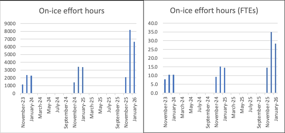
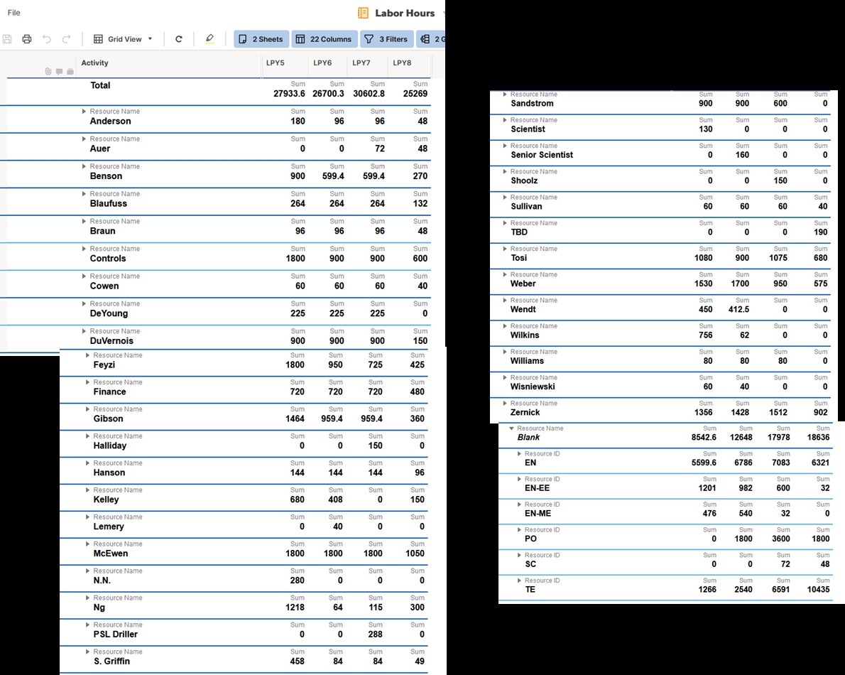
1 Can we see a forecast of resource usage histograms by month? See some of this information is in the Cost excel sheet but we did not see any slides showing critical resource usage, potential conflicts with key resources, etc.
#FTEs/month is the headcount / month, so really #FTE-Months/month.
For on-ice labor we use as reference a work week schedule of 6 days/week and 9 hours/day. A full season corresponds to 70 working days i.e., 70*9 = 630 working hours, with a maximum of 153 hours for the month of November, 234 hours for December and January. Below is a histogram of total # hours and equivalent FTEs and for on-ice work in FS1-2-3.
Additionally, we have looked at resource usage by named person (where available) or category of people. Below is the report from SmartSheets grouped by resource name/type.
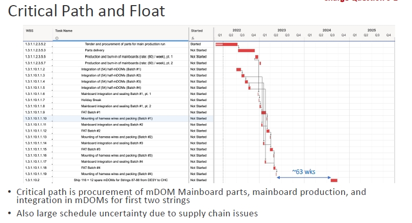
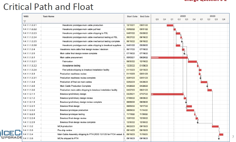
2 What is the critical path? There are bullets for critical items but no report on the critical path activities or the logical chain of activities driving project delivery or key milestones.
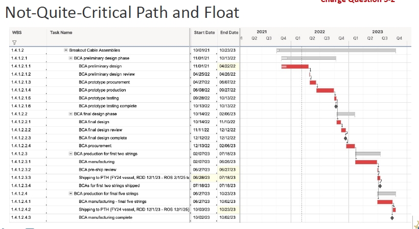
The critical path of getting pieces together to ship is shown below for 1.3 / 1.4 from the smart sheet schedule. The area we are watching carefully as it lies on the critical path is the drill control system (we just had a review of this a couple of weeks ago). The next item on the critical path is the main cable assemblies (here we have ~1 year of float before they must be shipped, however we were hoping to ship them in 2023). Finally, the mDOMs, while they currently have more than a year of float, because of problems procuring the parts for the main board we are looking at a redesign.
For on-ice activities, we have a detailed schedule in SmartSheets for each field season, and we suggest that we drill into that during the breakout sessions.
1.3:
1.4:
For 1.2

3 What is the planned value curve past 9/2021? We did not see anything showing this in detail beyond activities that are already completed or are very high-level planned expenditures by year.
Planned values by month for PY4 are as follows.
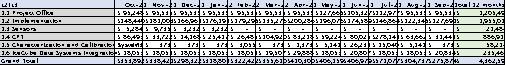
Planned values for PY5, 6, 7 and 8 are as listed in this folder:
https://docushare.icecube.wisc.edu/dsweb/View/Collection-16477
Data are in Smartsheets but have not been tabulated by month yet. We will do this shortly after the review and forward.
4 Does the Project have a resource to support schedule development and maintenance? If so, how much time is allocated?
We have a contractor (Jim Lowe) for 50%. We have an open position vacancy listing to add a full-time project controls person (replacing Marek Rogal) to the WIPAC team.
5 What is the prioritization of instruments/components to be installed on the IC/U strings? From the presentations, it was clear that there are a number of calibration and primary instruments planned to be installed on each string, and the extent to which one or another instrument kind of instrument achieves the necessary goals. However, it is not clear what happens if, say, the project is only able to install three of the seven strings, or if any one of these calibration instruments is not provided on time, or budget overruns require descoping in advance of the final deployment year. We would like to see a prioritized list of how critical each hole and individual instruments are to the project's success, and what are descope options/alternatives for each.
The most important components to the Upgrade science goal are the primary photosensors (mDOMs and D-Eggs, with pDOMs), which are necessary for the oscillation science goals and also contain substantial calibration instrumentation (flashers, cameras, inclinometers, and compasses). The POCAM and PencilBeam devices have unique, complementary calibration capabilities and deploying at least one of each per string is of primary importance to the calibration program. Deploying at least one acoustic module and Sweden Camera per string are next in priority. It should be noted that missing instrumentation on the strings at pre-assigned breakout positions will need to be replaced with spacers. Note, all of the standalone calibration devices are being developed by separate teams so they do not impact each others’ schedules.
“Special devices” (R&D Modules) in WBS 1.3 are not critical to the primary science goals of the Upgrade. These should not be confused with the calibration devices.
The most likely descope decision scenarios will be taking place in field season 3:
· The first option for descoping is to forego the cold ream stage to mitigate hole ice bubble formation (downscope option 2). We are confident in our ability to measure the properties of any hole ice that forms with the extensive camera and flasher system and updated photosensors.
· The next option of descoping is to reduce the number of strings, e.g., to 6 or 5 (down scope option 1). Individual strings are not very different from each other except that some boreholes are deeper, measuring the properties of the deep ice (below the IceCube instrumented volume) is an important goal of the Upgrade. The dust logger should be operated on a deep borehole in order to get precise measurement of the dust properties of the deep ice. If fewer strings are to be deployed, shifting more calibration instrumentation onto these strings would be considered to mitigate the effects of fewer holes.
The exact sequencing of the string drill order in case of a 6 or 5 (or fewer) string descope scenario has yet to be developed. It requires us to balance science and drill sequence considerations.
There is a presentation explaining the scope management options described in the scope management plan available.
6 RE 1.3:
6.1 Can we be given access to the Final Design Review reports from the April 2022 mDOM FDR and the ICM FDR?
The mDOM FDR report and the reports from the ICM reviews, including a link separate link to the material from the ICM Golden Image firmware review, have been posted to DocuShare Q&A. For the ICM separate reviews have been conducted for the hardware design and the firmware.
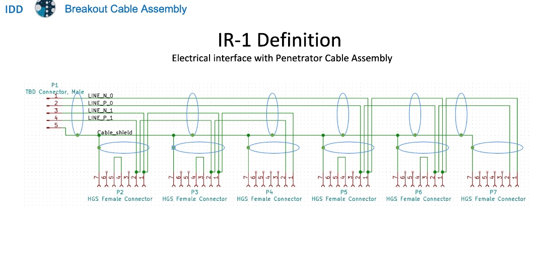
6.2 Can we be given access to the electrical ICD between the Main Cable and Penetrator Assemblies?
The Main Cable Assembly connects to a DOM’s Penetrator Cable Assembly via an intermediate cable called the Breakout Cable Assembly (BCA), which is currently in development. Interfaces in the upgrade project are defined as engineering requirements and described in each item’s “Interface Definition Document” (IDD), where all external interfaces are listed and each interface is specified in detail. An excerpt from the draft BCA IDD is provided below: The draft BCA IDD document has also been uploaded to the folder.
7 RE 1.4:
7.1 What fault conditions can cause an unrecoverable use of a string or DOM? Have such failures occurred in IceCube Gen 1? Are there features of the Upgrade Comms/Power/Timing systems that would increase the probability of such events?
Gen1 had no string failures. There are no modifications to the CPT plan for the ICU that increase the risk of string-level failure appreciably. There were some initial DOM failures in Gen1 (see plot below) during freeze-in, Later jumps are single DOM losses of unknown cause.
Some modules were believed to have suffered partial loss of function (local coincidence) from ESD damage. This was determined to be caused by human error (skipped ground strap installation step in main cable prep procedure), coupled with insufficient ESD protection on local coincidence lines of DOMs.
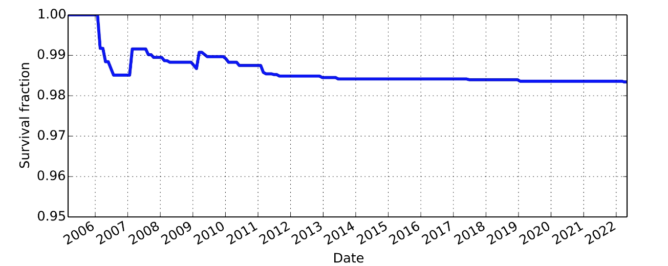
Gen1 DOM Survival fraction as a function of time
.
String and module level failures are examined in the in-ice device & string FMEA (will show this in the breakout session). In essence, the main failure modes for modules are electronics problems which we mitigate primarily with three levels of effort: (1) in the design phase, parts selections are made in accordance with an understanding of the physics of failure for these parts, using conservative temperature and voltage ratings, and automotive (at a minimum) specification, (2) board manufacturing using best practices and HALT plus HASS testing of board assemblies, and (3) extensive testing of integrated modules (during the Final Acceptance Testing, FAT) for extended operations of the modules over temperature cycles, operating cycles, reprogramming cycles, and corner testing.
CPT-related mechanical fault conditions associated with loss of a single DOM are primarily PCA outboard connector failure and penetrator seal failure at pressure vessel. The PCA is a new design, but overall risk is comparable to Gen1. Numerous outboard connector failures ("wet connector”) were observed in Gen1. Note that "wet connectors” limit ability to power DOMs prior to freeze-in, but generally do not lead to loss of DOM after freeze-in, as ice is not conductive. The ICU PCA connector was redesigned with stainless steel body rather than glass-reinforced epoxy and with o-ring seal to improve reliability. Penetrator body design is similar to Gen1 and has been pressure-tested both independently and as integrated with both mDOM and DEgg pressure vessels. No failures were observed, but a minor modification of the penetrator body was made as a result of the testing to improve the mating to the pressure vessels. DOM attachment/deployment procedures are similar to Gen1 and no increased risks are foreseen.
One difference from Gen1 is the introduction of the BCA, connecting 4-6 devices (depending on the quad) to a single main cable breakout. BCAs are similar to the 17m penetrator pigtails used in Gen1, but with multiple connectors. No failures were associated with the long pigtails or with the main cable breakout connections in Gen1. As noted above, ICU connectors were redesigned for additional robustness compared to Gen1, and connector leakage is generally not associated with loss of instrumentation in any case. In principle the connection of multiple DOMs to a single BCA could lead to stress associated with differential DOM motion during freeze-in, but the BCAs are designed with considerable slack to protect against such effects. The introduction of the BCA is thus not believed to increase risk of unrecoverable loss of DOMs in ICU.
Mechanical failure modes associated with loss of an entire string are registered in the FMEA. As noted above, no string failures occurred in Gen1. Differences from Gen1 that could increase risk are quantity (3) instead of (2) DOMs per wirepair, longer deployment times, harness-harness load bearing in physics region, and a greater variety of deployed instruments. We anticipate that the ICU main cable will be a composite design (to be discussed in the breakout session), but this design incorporates substantially more load-bearing aramid fiber, which will be less disrupted during installation of breakout terminations compared to Gen1, and the cable will be tested to mechanical loads 5x the maximum working load during the design review process.
7.2 What is the production test procedure for the MCA or BCA? Are there significant differences from Gen 1 cable tests? May we see a document describing the test protocol or test report?
The cable production tests are based on Gen1 procedures. Contracts for MCA and BCA production have not yet been issued so test procedures and sample reports are not yet finalized. Analogous documentation for the PCAs is attached for reference.
Main cable production test protocol, as specified in the RFP:
Continuity test: Electrically verify that each conductor is connected to the correct pin on the external and (if applicable) internal connectors
Isolation test: For each conductor, ground all other conductors and shield together, and verify that the conductor under test is electrically isolated from the rest.
Insulation resistance test: For each conductor, ground all other conductors and shield together, place 800V DC between these two circuits, and monitor the resistance of the insulation after one minute. Record the final value, it should be stable and at least 1 MΩ
Complete Crosstalk Test: NEXT and ELFEXT shall be measured from 100 kHz to 10 MHz at a minimum of 50 equally spaced frequencies on a logarithmic frequency scale. Attenuation and impedance shall be measured from 100 kHz to 10 MHz at a minimum of 5 equally spaced frequencies on a logarithmic frequency scale, including a measurement at 1.0 MHz.
Abbreviated Crosstalk Test: NEXT and ELFEXT shall be measured at 2.0 MHz.
Complete crosstalk test is performed on the first article or qualification sample; abbreviated test is performed on each production unit. Continuity, isolation and insulation resistance tests are performed before and after installation of breakout terminations. Mechanical tests (pull and pressure tests) will be conducted on prototypes only.
BCA (and PCA) electrical test protocol, performed on each unit:
Continuity test: Electrically verify that each conductor is connected to the correct pin on the external and (if applicable) internal connectors
Isolation test: For each conductor, ground all other conductors and shield together, and verify that the conductor under test is electrically isolated from the rest.
Insulation resistance test: For each conductor, ground all other conductors and shield together, place 500V DC between these two circuits, and monitor the resistance of the insulation after one minute. Record the final value, it should be stable and at least 1 MΩ.
As an example, a list of the production quality checkpoints and a sample test certificate from the PCAs are included (HGS PCA QC checkpoints list and a sample test report).
8 RE 1.6:
8.1 How is GPS timing implemented since satellites are not consistently visible from South Pole?
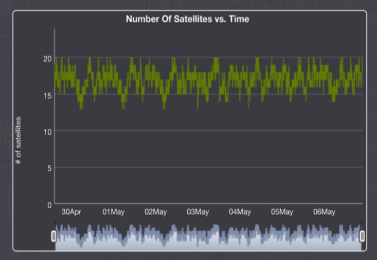 The typical number of satellites (GPS and GLONASS) in view at Pole is 15-20 after altitude masking (see Figure below). The Upgrade will use the existing IceCube GPS (Spectracom SecureSync) as the master clock. This clock contains an oven-compensated crystal oscillator which will continue to operate undisciplined if GNSS signal integrity is compromised, albeit with increasing drift (typ df/f ~ 10-10 over 1 day). This does not affect the relative timing between modules and thus would not compromise the observatory operation except for extremely long outages of order months.
Perhaps there is a misunderstanding of the IceCube timing system architecture. The MC 10 MHz signal is fanned out to each IceCube and IceCube Upgrade DOMHub/FieldHub : at this level the system is synchronous and even if the clock had some high level of phase noise the channel-to-channel timing would still be accurate to the ns-level even if the timing relative to UTC/GPS is off by a large amount. Of course, at the second or millisecond level we use this time to determine coincidence with astronomical events so we would like to be as precise as possible here too, especially in timing the neutrino shockwave from a galactic supernova, microsecond scale accuracy would be advantageous.
9 RE Management: please provide the panel an example showing how technical subsystem requirements flow down and are traceable from higher-level science requirements.
An example: The LED flasher brightness range as specified in the flasher ERD is 5e6 – 1e9 photons per flash. The upper part of the brightness range, from 5e7 to 5e9 photons, is based on simulation studies which show that this yields 100 p.e. detected per receiving module on the neighboring strings, up to 100m away, which is necessary for the required measurement of ice properties. Lower end values work well for receivers 40m away and in the bright part of the LED's illumination field. Extension of the dynamic range down to 5e6 allows measurement of timing offsets (PMT transit time and electronics effects in RAPCAL or otherwise) by flashing between neighboring DOMs on the same string.
Timo Karg additionally presented the sensor design parameters study linked in his breakout talk.
10 RE Cost/Risk: are there any risks assigned for loss of in-kind labor at universities and international collaborating institutions?
In-kind contributions from collaborating institutions, labor and equipment, have historically been very robust: as two examples, Japanese funding for D-Egg sensor contributions was committed months before the NSF award was made; and KIT procured 10,800 mDOM PMTs in PY2 as an additional contribution beyond what was foreseen in the proposal. Labor contributions are more difficult to quantify but have been nonetheless at or above the level required to support pledged scope. It should also be noted that these contributions have remained steadfast despite COVID delays and the past two years of Antarctic logistics planning uncertainty. We recognize however that this risk could play out as loss of key personnel required to complete technical scope (mDOM engineering, or software simulation leadership are examples that come to mind) and a risk should be entered into the RR to cover the possibility that collaborating institutions cannot quickly replace loss of such personnel.
11 RE: 1.2.10: Please outline plans regarding storage and temperature-controlled staging space for module unpacking, assembly and testing during Field Seasons 2 and 3?
The sensors’ storage temperature limit is –40C. During the summer, sensors will be stored outside, as in Gen1. Sensor boxes are designed so that a pre-perforated flap allows access to the penetrator without unpacking the sensor, similarly to Gen1.
At the point of origin, sensors are packed in pallets so that the penetrators can be accessed without unpacking the pallet. Once the sensors are delivered to Pole, pallets with sensors belonging to one string are loaded onto one sled (UHWM sheets fitted with AIPs). While the sensors are on the sled, the sled is driven into the testing tent (we have requested the use of the Solar Garage for this purpose) and penetrators are accessed to run the sensors through the South Pole Acceptance Testing Setup (this is all analog to what was done in Gen1). Once sensors are tested, the sled is carried to the DOM Handling Facility (DHF), parked next to the TOS, and the pallets are unloaded from the sled and loaded into the DOM Handling Facility. During installation the sensors are sorted and fed into the TOS/TOWER, with a buffer of half-dozen to a dozen sensors. Once the sensor gets in proximity to the hole it is lifted with the hoist and removed from the box. We plan to have two strings worth of sensors delivered to Pole by 12/15/2024. Ample time is allocated for these two strings to be tested during FS2 through the South Pole Acceptance Test Setup for these first two strings. After been tested these strings will be then stored in Cryo (only for winter), a plan which has been validated by ASC based on the volume of the sensors. In early summer the two string sensors will be taken out of Cryo. The 5 remaining strings will be delivered in FS3 and staged in a designated area near the cargo line, outside. Loading on sled and into the DHF will follow the same procedure as outlined above. At no point do we plan on assembling or reworking sensors at Pole. Spare sensors will be available to replace sensors not passing SPAT.
12 RE Logistics: Please make available in DocuShare the "IceCube Upgrade Logistics - Cargo Estimation and Shipment Planning" document.
Document posted in DocuShare in the logistics folder.
13 RE Project Office:
13.1 The project office schedule, cost, and risk tools (SmartTools, Excel, and @Risk) are not best practice choices of tools and require manual work (error prone?) to update various spreadsheets (e.g. population spreadsheet to level resources, float spreadsheet, costbook).
13.2 It is not clear if the project office has sufficient staff to support the PD and PM, with appropriate skills: cost estimating, scheduling, risk analysis and EVMS. An experienced PCS could fairly quickly convert the current schedule to use an integrated scheduling tool such as Primavera P6.
We made the choices we did in order to use a lightweight, collaborative tool suitable for a midscale, 5-year project. This allows the entire project team to interface with the schedule and cost workbook. We have a document that describes the tools in the docushare folder and how they comply with GAO best practices.
14 RE Schedule:
14.1 It is difficult for us to review the resource-loaded schedule, validate schedule logic integrity, explore the critical path/near critical paths, assess available float, etc. based on the information provided (e.g., PDF Gantt charts). A P6 file would be a lot easier.
14.2 The schedule is quantized with strict deadlines each year for ship-by dates and field seasons. It is imperative to systematically monitor the float before these deadlines allowing for the probability-weighted aggregated delays from all risks.
We are monitoring the float systematically.
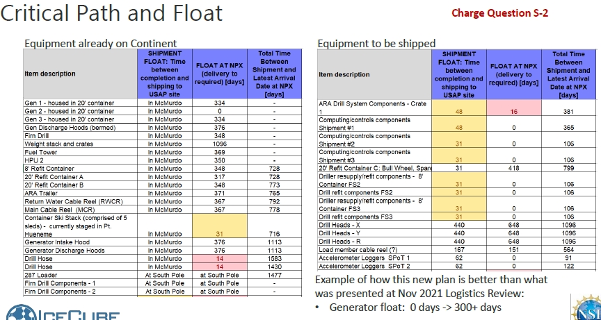
14.3 Float tables have many activities with very little or zero float – taken at face value this is very concerning.
Summary below. Ian/Delia will go through this in the breakout session. There are 48 shipments to SP with float below 20 days:
· 18 shipments are JIT as no SP environmentally controlled warehousing is available
· 6 shipments are dust logging equipment which is available for only one season
· 8 are vessel DNF/ComSur shipments for drill resupply
· 2 are accelerometer shipments that do not impact project deliverables
· 1 is Generator 2 where tasking at SP begins with offload of the container from Sled to Skiset when it arrives 12/1. Initial commissioning/testing is planned for December 5. Upon completion intake and exhaust ducts are installed and Gens/PDM relocated/positioned on SES pad and winterized (12/21/23)
· 3 shipments are DNF which have not yet had overwinter DNF storage space identified – likely that they can be expedited
· 4 shipments contain special devices whose schedule will be revised as the designs go through review. Most of the devices will be ready well in advance of shipment based but we have left completion date to be as late as possible.
· 4 shipments include sensors that are received and tested upon arrival at South Pole and then stored overwinter in Cryo
· 2 shipments include resupply for science.
15 RE Logistics: Presentation stated: “Float is calculated in the Cargo Master spreadsheet, rather than the SmartTools schedule.” It seems that there is not actually a master schedule that stores all schedule information in one coherent place – we find this a serious concern.
CM spreadsheet is needed for communication with AIL on a regular basis. It includes information such as weights, cubes, special handling, etc. that is essential for timely and effective communication. The float calculation is one aspect of the CM spreadsheet. It calculates float by subtracting dates that are directly coming from the master schedule. The CM spreadsheet is updated at least monthly and kept in synch with the master schedule.
16 RE Risk:
16.1 We could not find results of a stochastic schedule risk analysis with all risks. What are the top schedule risks? What are the various float values without risks, and then adjusted for risk at 80% CL? It is unclear how the sensitivity analysis presented during the Logistic section relates to the schedule risk analysis.
There is not a stochastic schedule risk analysis from the risk registry, only a cost analysis, we were unable to make a sensible quantitative analysis of the risk registry schedule risks. Note that a risk Monte Carlo is not required for an NSF midscale project. We have chosen to do this for the cost as we feel it is a useful metric of overall risk exposure. We have not done this for the schedule, and are managing aggressively to milestones.
Top schedule risks: winter storage failure could cause a year delay in worst cases. Similarly on-ice accidents have worst case schedule impacts of a full year. Critical drill system failures, or personnel casualties, during the FS3 can have impacts which exceed our project specifications or boundaries. That is, a risk which would have to be carried by the NSF.
We will show in the breakout session how logistics sensitivity analysis relates to schedule risk analysis. The sensitivity analysis is an attempt to analyze both the impacts of specific delays, and motivates examination of the on-ice activity network.
16.2 If we interpret Low/High cost exposure in the Risk Register as a flat range PDF, weight it by probability (middle of bin in register), and then sum over all risks, we get an expected mean total risk cost = Sum(P*mean cost impact) = $2.08M. This is much more than the $1.86M (at the higher 80% CL) shown in the presentation.
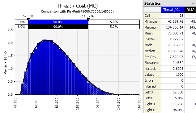
We are not sure exactly how the $2.08M was calculated: two of us independently arrived at $1.4M using your recipe. In our Monte Carlo calculation we used a PERT distribution for the low/high cost exposure, and excluded the NSF risk (TECH7, in red in the risk register) estimate. Note we have one opportunity in the register and we do include the logistics risks (in green) in the cost exposure, but also calculate with those removed for a comparison with the logistics sensitivity.
An example of a distribution for cost exposure is given below for “ORG2” [70000, 45000, 145000] [Major injury occurs during drill season, but not associated with drilling. Work stoppage occurs until review is performed and "safe to proceed" determined.]
16.3 The risk register is a good start but could be improved. Risks are classified in 5 fixed bins of probability – this should just be a percentage probability value. There are 5 bins per cost impact – this could just be specified as min/likely/max values. Same for schedule. The risks can still be binned for ranking purposes but storing P/impact values (not bins) retains information and facilitates risk aggregation. It is unclear what the Risk Exposure columns mean. Is the quantitative data complete?
These fixed bins are defined in the RIG (Research Infrastructure Guide), and we are following that guidance. We had noticed the coarseness of the binning, especially for the very low probabilities. We agree that maintaining our own probabilities and not relying on the RIG-suggested bins is a good idea and we will incorporate this in future revisions of the Risk Register.
Regarding the meaning of Risk Exposure: we have a quantitative estimate of a likely cost, first column of the risk exposure, along with estimates for potential low and high exposures. Many of the low/high estimates are less quantitative than the likely cost reflecting confidence in the likely estimate and also some possible best case and worst case scenarios.
16.4 Are risks associated to in-kind partner contributions systematically assessed and included as “handover” risks (cost impacts and delays) in the risk register and analysis?
Yes. They are assessed and included. We have risks for major in-kind deliverables. E.g., main cable assemblies are in-kind contributions. We have risks for both schedule delays and performance issues with the main cables.
17 When does the project expect to fill the scheduler position and what efforts will be made to maximize retention potential?
Applications are being received now. We expect to have interviews and a decision within 1-2 months. The retention strategy will be addressed within the context of long-term employment, superior benefits offered at UW-Madison, and potential for close and direct collaboration with top-notch technical staff.
18 We heard evidence of “bottom-up” cost basing. Has any “top-down” cost estimation been performed?
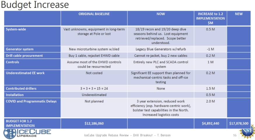
Slide 16 of the drill breakout talk shows a breakdown of cost increase from original baseline to today’s rebaseline. This is an example of a recent top-down look to rationalize the cost increase in WBS 1.2. See thumbnail of the slide below. We can go through this together during the drill breakout, the cost/schedule session, or both.
19 How does the project determine the impact of missed in-kind contributions?
Some of these are in the risk register explicitly. The in-kind contributions are all in the schedule and are reflected in the milestones. It is only in the costs for which the handling of on-project and off-project contributions differ.
20 Once sensors are deployed, are there mitigation plans if calibration activities do not fully materialize?
Dust logging can only occur before string deployment in a borehole that has not yet frozen. We do have multiple calibration devices in place (I.e., flashers) which can cross-check the dust logger and if the dust logging does not occur, we will still be able to make a measurement but it will be less precise. If post-deployment and/or off-ice calibration activities are delayed past the end of the project, they will need support from M&O or in-kind contributions.
21 We are concerned that the scheduling tools we have been presented are primarily for the panel’s benefit rather than being developed to internally manage the project.
The SmartSheet schedule is updated by all of the L2s on a monthly basis, checking milestones and evaluating percent completes. Each of them uses SmartSheets cooperatively and remotely using this Cloud-based resource. Output from the Schedule is used for calculating EV metrics and reported monthly in the NSF monthly report.
The cargo master spreadsheet is not automatically connected to the master schedule, but all cargo handling is managed by the logistics manager who maintains the cargo spreadsheet.