-1 TeV -1 s -2 cm -12 x 10
Residuals
Events
WIMP mass [GeV/c
Spin−independent cross section [cm
3 10

A Maximum-Likelihood Search for Neutrino Point Sources with the

AMANDA-II Detector

James R. Braun

A dissertation submitted in partial fulfillment of the

requirements for the degree of

Doctor of Philosophy

(Physics)

at the

University of Wisconsin – Madison

2009

A Maximum-Likelihood Search for Neutrino Point

Sources with the AMANDA-II Detector

James R. Braun

Under the supervision of Professor Albrecht Karle

At the University of Wisconsin — Madison

Neutrino astronomy offers a new window to study the high energy universe. The AMANDA-II

detector records neutrino-induced muon events in the ice sheet beneath the geographic South Pole,

and has accumulated 3.8 years of livetime from 2000 – 2006. After reconstructing muon tracks

and applying selection criteria, we arrive at a sample of 6595 events originating from the Northern

Sky, predominantly atmospheric neutrinos with primary energy 100 GeV to 8 TeV. We search these

events for evidence of astrophysical neutrino point sources using a maximum-likelihood method. No

excess above the atmospheric neutrino background is found, and we set upper limits on neutrino

fluxes. Finally, a well-known potential dark matter signature is emission of high energy neutrinos

from annihilation of WIMPs gravitationally bound to the Sun. We search for high energy neutrinos

from the Sun and find no excess. Our limits on WIMP-nucleon cross section set new constraints on

MSSM parameter space.

Albrecht Karle (Adviser)

Acknowledgments

I owe a debt to many for the support, advice, and friendship I’ve received and made this work

possible.

Particularly, I offer thanks to my adviser Albrecht Karle for his support, for suggesting neu-

trino point sources and dark matter as fruitful research topics with AMANDA, and for his advice

throughout my work. I offer thanks to Bob Morse for my initial interest in AMANDA and IceCube,

and to Francis Halzen for sharing his advice and his attitude toward science.

I wish to thank Gary Hill and Chad Finley for many discussions regarding maximum-likelihood

techniques and point source analysis. I also thank Kael Hanson and Chris Wendt for the technical

skills I’ve learned working on DOM testing and calibration.

Many thanks to Mark Krasberg for many softball games and sailing trips, and for making the

workplace more fun. I thank my office mate John Kelley for nearly always having the answers to my

questions and introducing me to the delicious wonders of good coffee.

I wish to thank my parents, Jim and Chris, my grandfather, Ralph, and my uncle, Steve,

for encouraging my interest in Science over all these years. Finally, I thank my fianc´ee Jess for her

unyielding love and support throughout this work.

Contents

Acknowledgments

1 The High Energy Universe

1.1 CosmicRays . . . . . . . . . . . . . . . . . . . . . . . . . . . . . . . . . . . . . . . . .

1.1.1 Cosmic Ray Flux and Composition . . . . . . . . . . . . . . . . . . . . . . . . .

1.1.2 CosmicRayEnergization . . . . . . . . . . . . . . . . . . . . . . . . . . . . . .

1.1.3 Candidate Cosmic Ray Accelerators . . . . . . . . . . . . . . . . . . . . . . . .

1.2 Cosmic Ray Interaction with Matter and Radiation . . . . . . . . . . . . . . . . . . . .

1.2.1 ChargedParticles. . . . . . . . . . . . . . . . . . . . . . . . . . . . . . . . . . .

1.2.2 Photons . . . . . . . . . . . . . . . . . . . . . . . . . . . . . . . . . . . . . . . .

1.2.3 Neutrinos . . . . . . . . . . . . . . . . . . . . . . . . . . . . . . . . . . . . . . . 10

1.3 CosmicRayAirShowers . . . . . . . . . . . . . . . . . . . . . . . . . . . . . . . . . . . 10

1.3.1 ElectromagneticShowers . . . . . . . . . . . . . . . . . . . . . . . . . . . . . . 10

1.3.2 HadronicShowers . . . . . . . . . . . . . . . . . . . . . . . . . . . . . . . . . . 10

1.3.2.1 Atmospheric Muons and Neutrinos . . . . . . . . . . . . . . . . . . . . 12

1.4 HighEnergyAstronomy . . . . . . . . . . . . . . . . . . . . . . . . . . . . . . . . . . . 13

1.4.1 ChargedParticles. . . . . . . . . . . . . . . . . . . . . . . . . . . . . . . . . . . 14

1.4.2 Photons . . . . . . . . . . . . . . . . . . . . . . . . . . . . . . . . . . . . . . . . 15

2 High Energy Astronomy with Neutrinos

2.1 NeutrinoInteraction . . . . . . . . . . . . . . . . . . . . . . . . . . . . . . . . . . . . . 18

2.2 LeptonPropagation . . . . . . . . . . . . . . . . . . . . . . . . . . . . . . . . . . . . . 19

iii

2.2.1 Electrons . . . . . . . . . . . . . . . . . . . . . . . . . . . . . . . . . . . . . . . 21

2.2.2 Muons. . . . . . . . . . . . . . . . . . . . . . . . . . . . . . . . . . . . . . . . . 21

2.2.3 TauParticles . . . . . . . . . . . . . . . . . . . . . . . . . . . . . . . . . . . . . 22

2.3 TeVNeutrinoDetection . . . . . . . . . . . . . . . . . . . . . . . . . . . . . . . . . . . 22

2.3.1 CherenkovRadiation. . . . . . . . . . . . . . . . . . . . . . . . . . . . . . . . . 22

2.3.2 Energy Resolution Considerations . . . . . . . . . . . . . . . . . . . . . . . . . 23

2.3.3 Angular Resolution Considerations . . . . . . . . . . . . . . . . . . . . . . . . . 24

2.4 The EarthasaNeutrinoTarget. . . . . . . . . . . . . . . . . . . . . . . . . . . . . . . 24

2.5 The Background from Cosmic Ray Air Showers . . . . . . . . . . . . . . . . . . . . . . 25

3 The AMANDA Cherenkov Telescope

3.1 In-IceArray. . . . . . . . . . . . . . . . . . . . . . . . . . . . . . . . . . . . . . . . . . 28

3.2 Muon-DAQ . . . . . . . . . . . . . . . . . . . . . . . . . . . . . . . . . . . . . . . . . . 30

3.3 Calibration . . . . . . . . . . . . . . . . . . . . . . . . . . . . . . . . . . . . . . . . . . 31

3.4 PropertiesofSouthPoleIce . . . . . . . . . . . . . . . . . . . . . . . . . . . . . . . . . 33

3.4.1 Glacial Ice atthe South Pole . . . . . . . . . . . . . . . . . . . . . . . . . . . . 33

3.4.2 HoleIce . . . . . . . . . . . . . . . . . . . . . . . . . . . . . . . . . . . . . . . . 33

3.5 Simulation. . . . . . . . . . . . . . . . . . . . . . . . . . . . . . . . . . . . . . . . . . . 33

4 Data Selection and Event Reconstruction

4.1 DataSelection . . . . . . . . . . . . . . . . . . . . . . . . . . . . . . . . . . . . . . . . 36

4.2 HitSelection . . . . . . . . . . . . . . . . . . . . . . . . . . . . . . . . . . . . . . . . . 39

4.3 TrackReconstruction. . . . . . . . . . . . . . . . . . . . . . . . . . . . . . . . . . . . . 40

4.3.1 Unbiased Likelihood Reconstruction . . . . . . . . . . . . . . . . . . . . . . . . 41

4.3.2 Paraboloid Reconstruction. . . . . . . . . . . . . . . . . . . . . . . . . . . . . . 44

4.3.3 Forced Downgoing (Bayesian) Reconstruction . . . . . . . . . . . . . . . . . . . 44

4.3.4 FirstGuessAlgorithms . . . . . . . . . . . . . . . . . . . . . . . . . . . . . . . 46

4.3.4.1 DirectWalk . . . . . . . . . . . . . . . . . . . . . . . . . . . . . . . . 47

4.3.4.2 JAMS. . . . . . . . . . . . . . . . . . . . . . . . . . . . . . . . . . . . 47

5 Event Selection

5.1 DataSets . . . . . . . . . . . . . . . . . . . . . . . . . . . . . . . . . . . . . . . . . . . 48

5.2 Filtering DowngoingEvents . . . . . . . . . . . . . . . . . . . . . . . . . . . . . . . . . 50

5.2.1 Retriggering. . . . . . . . . . . . . . . . . . . . . . . . . . . . . . . . . . . . . . 50

5.2.2 First Guess Reconstruction . . . . . . . . . . . . . . . . . . . . . . . . . . . . . 50

5.2.3 Unbiased Likelihood Reconstruction . . . . . . . . . . . . . . . . . . . . . . . . 51

5.3 FinalEventSelection. . . . . . . . . . . . . . . . . . . . . . . . . . . . . . . . . . . . . 51

6 Search Method

6.1 Maximum Likelihood Search Method . . . . . . . . . . . . . . . . . . . . . . . . . . . . 59

6.1.1 Confidence Level and Power of a Test . . . . . . . . . . . . . . . . . . . . . . . 59

6.1.2 SearchMethod . . . . . . . . . . . . . . . . . . . . . . . . . . . . . . . . . . . . 60

6.1.2.1 SpatialLikelihood . . . . . . . . . . . . . . . . . . . . . . . . . . . . . 60

6.1.2.2 EnergyLikelihood . . . . . . . . . . . . . . . . . . . . . . . . . . . . . 61

6.1.2.3 Signal and Background PDFs and the Test Statistic . . . . . . . . . . 62

6.2 Evaluating Significance and Discovery Potential . . . . . . . . . . . . . . . . . . . . . . 64

6.3 EvaluatingFluxLimits. . . . . . . . . . . . . . . . . . . . . . . . . . . . . . . . . . . . 66

6.4 EstimatingSpectralIndex . . . . . . . . . . . . . . . . . . . . . . . . . . . . . . . . . . 68

7 Search for Neutrino Point Sources

7.1 Systematic Uncertainties . . . . . . . . . . . . . . . . . . . . . . . . . . . . . . . . . . . 70

7.1.1 Optical Module Sensitivity . . . . . . . . . . . . . . . . . . . . . . . . . . . . . 70

7.1.2 PhotonPropagation . . . . . . . . . . . . . . . . . . . . . . . . . . . . . . . . . 71

7.1.3 Event Selection and Reconstruction . . . . . . . . . . . . . . . . . . . . . . . . 71

7.1.4 Rock Density, Neutrino Cross Section, and Other Sources of Uncertainty . . . . 72

7.2 SearchforPointSources . . . . . . . . . . . . . . . . . . . . . . . . . . . . . . . . . . . 72

7.2.1 Search Based on a List of Candidate Sources . . . . . . . . . . . . . . . . . . . 72

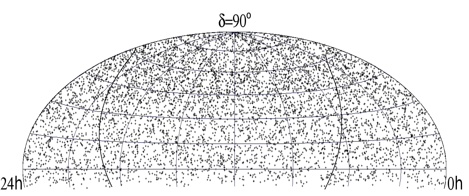
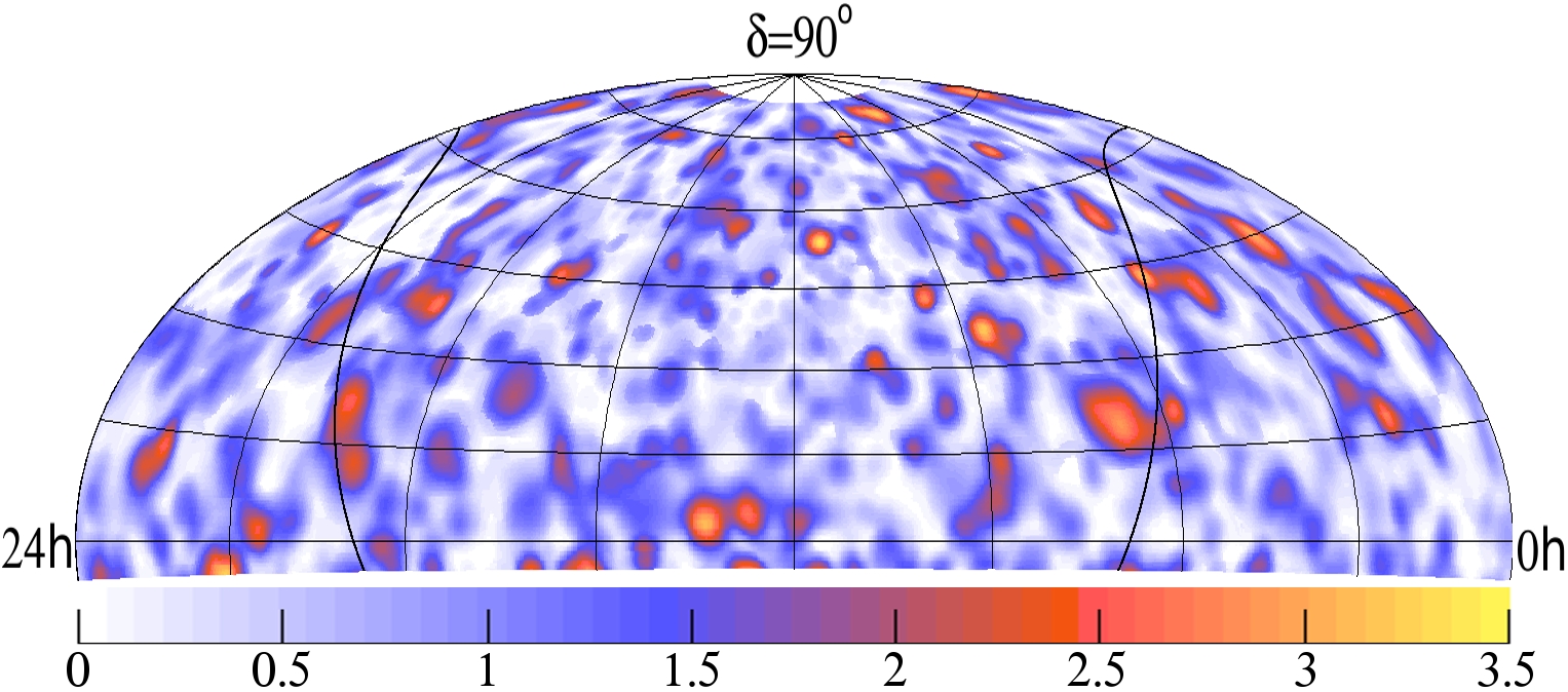
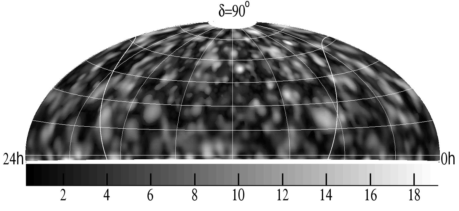
7.2.2 Searchofthe NorthernSky . . . . . . . . . . . . . . . . . . . . . . . . . . . . . 73

7.2.3 TheCygnusRegion . . . . . . . . . . . . . . . . . . . . . . . . . . . . . . . . . 73

7.2.4 MilagroSourceStacking . . . . . . . . . . . . . . . . . . . . . . . . . . . . . . . 73

7.2.5 Search for Event Correlations at Small Angular Scales . . . . . . . . . . . . . . 78

8 Search for WIMP Dark Matter from the Sun

8.1 Detection ofWIMP DarkMatter . . . . . . . . . . . . . . . . . . . . . . . . . . . . . . 80

8.2 Solar WIMP Search with AMANDA . . . . . . . . . . . . . . . . . . . . . . . . . . . . 82

8.2.1 Solar WIMP Signal Simulation . . . . . . . . . . . . . . . . . . . . . . . . . . . 83

8.2.2 SearchResults . . . . . . . . . . . . . . . . . . . . . . . . . . . . . . . . . . . . 84

8.2.3 Limits on Neutrino-Induced Muon Fluxes and WIMP-Nucleon Cross Sections . 86

9 The Future

9.1 IceCube . . . . . . . . . . . . . . . . . . . . . . . . . . . . . . . . . . . . . . . . . . . . 94

9.1.1 IceCube Digital Optical Modules . . . . . . . . . . . . . . . . . . . . . . . . . . 94

9.1.2 IceCube DeepCore Extension . . . . . . . . . . . . . . . . . . . . . . . . . . . . 97

A Weighting Simulated Events

108

A.1 Weighting Neutrino Simulation . . . . . . . . . . . . . . . . . . . . . . . . . . . . . . . 108

A.2 NeutrinoEffectiveArea . . . . . . . . . . . . . . . . . . . . . . . . . . . . . . . . . . . 110

A.3 EffectiveVolume . . . . . . . . . . . . . . . . . . . . . . . . . . . . . . . . . . . . . . . 112

A.4 Spectrally Averaged Effective Areas and Volumes . . . . . . . . . . . . . . . . . . . . . 113

B Time-Dependent Search for Point Sources

114

B.1 Flares or Bursts with an Assumed Time Dependence . . . . . . . . . . . . . . . . . . . 114

B.2 Flares or Bursts with an Unknown Time Dependence . . . . . . . . . . . . . . . . . . . 115

B.2.1 Test Statistic and Approximation of the Likelihood Function . . . . . . . . . . 116

B.3 PeriodicSources . . . . . . . . . . . . . . . . . . . . . . . . . . . . . . . . . . . . . . . 117

Chapter 1

The High Energy Universe

Within our known universe are components which are hidden or poorly understood. One such

component is associated with the high energy cosmic ray particles which bombard Earth, including

particles many orders of magnitude more energetic than those generated by LHC or other collider

experiments. The sources of cosmic rays are generally unknown; however, the existence of such

particles implies extreme particle accelerators must exist in the universe. Further study of cosmic

rays, including neutrino astronomy, will improve our knowledge of this high energy universe and

potentially reveal the cosmic ray sources.

1.1 Cosmic Rays

The existence of an energetic ionizing radiation at Earth’s surface had been established near

the beginning of the 20

century, as several scientists observed that charged, isolated electroscopes

slowly discharge with time. The pioneering work establishing cosmic radiation was performed by

Hess in 1911-1912, during several high altitude balloon flights. Hess observed the rate of electroscope

discharge increases with altitude, establishing that the radiation source is extraterrestrial. The work

was published in 1912 [1] and earned Hess a Nobel Prize in 1936.

1.1.1 Cosmic Ray Flux and Composition

The measured cosmic ray flux spans an enormous energy range, stretching to 10

eV and

falling roughly with an E

? 2 . 7

power law above ∼ 1 GeV. The measured cosmic ray spectrum above

10 TeV is shown in figure 1.1, multiplied by E

2 . 7

. At relatively low energies, below ∼ 1 PeV, cosmic

Grigorov

JACEE

MGU

TienShan

Tibet07

Akeno

CASA/MIA

Hegra

Flys Eye

Agasa

HiRes1

HiRes2

Auger SD

Auger hybrid

Kascade

[eV]

2.7

(

) [GeV

1.7

−

]

Ankle

Knee

2nd Knee

Figure 1.1: Cosmic ray flux measurements of an ensemble of experiments, from [2].

The flux is multiplied by E

2 . 7

to enhance the spectral features.

rays are directly measured by spectrometers ( ? TeV) and particle calorimeters in orbit (e.g. [3, 4]),

or in long-duration stratospheric balloon flights (e.g. [5, 6]) above most of the atmosphere. At higher

energies, detectors with progressively larger acceptance are required to offset the sharply falling flux

with energy. Such acceptance is provided by recording the cascades produced as cosmic rays enter the

atmosphere (section 1.3). At the highest energies, these cascades are recorded by giant ground-based

air shower detectors [7], atmospheric fluorescence telescopes [8], or both [9]. Above 10

eV, statistics

rapidly diminish. Several features are apparent in the energy spectrum. At ∼ 3 PeV the spectrum

steepens, a feature known as the “knee”, and hardens again at the ∼ 3 EeV “ankle”. These features

provide clues to cosmic ray origins; particularly, it is believed that the ankle represents a transition

from galactic cosmic rays to those produced by more powerful extragalactic sources. Above ∼ 60 EeV

the spectrum again steepens [10, 11]. This steepening is evidence of the GZK cutoff [12], discussed

E [eV]

]

−1

−2

(E) [GeV cm

−7

−6

AMANDA (2007)

AMANDA UHE (2008)

AUGER (2008)

ANITA (2008)

FORTE (2004)

Figure 1.2: Current limits on E

? 2

all-flavor neutrino cosmic ray fluxes above 10 TeV

further in section 1.2.

Cosmic rays are primarily composed of hadronic particles, generally protons and heavier nuclei.

The ratio of these constituent nuclei is currently an active area of research, and significant uncertainty

exits at high energies [13, 14]. The flux of hadronic cosmic rays is very nearly isotropic at Earth due

to magnetic scrambling from galactic and extragalactic magnetic fields. A small (0.1%) anisotropy

exists in arrival directions at ∼ TeV energies [15, 16, 17], possibly due to the local magnetic field

or a nearby cosmic ray source. Below ∼ 100 TeV, a small fraction of cosmic rays are known to be

photons, and, since photons are not deflected by magnetic fields, many TeV photon sources have been

discovered [18, 19, 20]. Many of these TeV photon sources are candidate sources of hadronic cosmic

rays. At ∼ TeV energies and below, electrons and positrons constitute a small fraction of cosmic rays.

Measurements of cosmic ray electrons and positrons [21, 22, 23, 24] and positron fraction [25] may

provide evidence for WIMP dark matter, discussed further in chapter 8. No neutrino component of

cosmic rays has yet been discovered [26, 27, 28, 29, 30, 31, 32, 33, 34, 35]. Flux limits on this neutrino

component above 10 TeV are shown in figure 1.2.

1.1.2 Cosmic Ray Energization

The mechanisms thought to generate high energy cosmic rays are grouped in two categories.

• The top-down scenario : Supermassive particles with long lifetimes decay, producing cosmic

rays energized by the rest mass of the parent particle.

• The bottom-up scenario : Low energy particles in the vicinity of energetic astrophysical

phenomena are energized and propagate to Earth as cosmic rays.

Sources of supermassive particles in top-down models include super-heavy dark matter [36, 37] and

topological defects [38]. Many top-down models are largely constrained. Models suggesting that

ultra-high energy cosmic rays (UHECR) are produced locally in the galactic halo are constrained

by observations of the GZK cutoff, discussed in section 1.2, and by measurements of the cosmic ray

photon fraction [39, 40]. Top-down UHECR models at cosmological distances are constrained by

limits on ultra-high energy neutrino fluxes and the diffuse GeV galactic photon flux [41].

The most widely accepted bottom-up acceleration mechanism is Fermi acceleration [42]. In

first order Fermi acceleration, charged particles are energized by interactions with relativistic shocks.

Such particles are confined to the shock by magnetic inhomogeneities and are energized by repeated

magnetic reflection through the shock front. The repeated energization creates nonthermal, power

law spectra with indices

? E

? γ

;

γ ≥ 2.

(1.1)

Charged particles can no longer be confined to the shock when the particle gyroradii approach the

geometric size of the shock; therefore, the maximum energy attainable is a function of magnetic field

strength and source size:

⊥

E/c

ZeB

⊥

(1.2)

max

GeV

? 3 × 10

? 2

× Z ×

(1.3)

Figure 1.3, originally produced by Hillas [43], illustrates the source sizes and magnetic fields necessary

to generate the highest energy cosmic rays, along with the estimated size and magnetic field for several

classes of astronomical objects.

1.1.3 Candidate Cosmic Ray Accelerators

From the Hillas diagram in figure 1.3, several classes of energetic objects have the potential to

accelerate cosmic rays to ∼ PeV energies and beyond. Some of the most important include:

(100 EeV) 

(1 ZeV) 

Neutron 

star 

White 

dwarf 

Protons 

GRB

Galactic 

disk 

halo 

galaxies 

Colliding 

jets 

nuclei 

lobes 

hot−spots 

SNR

Clusters 

galaxies 

active 

1 au   1 pc 1 kpc 1 Mpc 

−9 

−3 

3

9

15

3  6  9  12  15  18 21 

log(Magnetic field, gauss) 

log(size, km) 

Fe (100 EeV) 

Protons 

Figure 1.3: ’Hillas diagram’ of source sizes and magnetic fields necessary to accelerate

EeV cosmic rays, including the sizes and estimated magnetic fields for several classes

of astronomical objects, from [44].

• Active Galactic Nuclei (AGN) : Active galaxies are significant sources of nonthermal radi-

ation, thought to be powered by matter accretion on a central supermassive black hole. AGN

are extensively classified based on the presence of relativistic jets, radio luminosity, x-ray lu-

minosity, and other criteria [45]. Importantly, the nonthermal keV x-ray emission observed

from some AGN is likely synchrotron radiation from shock accelerated electrons and indicates

potential for hadron acceleration. Several AGN are known TeV photon emitters [46]. The TeV

flux is variable in time, with occasional flaring on timescales of ∼ days often linked to flares in

nonthermal x-rays (e.g. [47]).

• Gamma Ray Bursts (GRBs) : GRBs are short (10

? 3

s – 10

s [48]), highly energetic (E

> 10

erg) bursts of keV – MeV photons from cosmological distances. The radiation is believed

to be beamed along an expanding ultra-relativistic fireball [49] with a Lorenz factor of 100-1000

[50]. Similar to AGN, the keV – MeV emission is thought to be synchrotron emission from

shock accelerated electrons.

• Microquasars : Microquasars are potential galactic sources with relativistic jets similar to

AGN, except microquasars are much smaller; the central engine is a neutron star or black hole

up to a few stellar masses. Several microquasars are significant TeV photon sources [46], and

many are bright x-ray sources.

• Supernova Remnants (SNRs) : Supernovae are the most powerful explosions known in our

galaxy, and the relativistic shocks produced expand for many years and are a possible cosmic ray

acceleration source. SNRs can be broadly classified into two categories: Those with a central

pulsar producing a relativistic wind (PWN), including the Crab, and those which are shell-like,

including Cas A, with the latter type often considered the most likely source of Galactic cosmic

rays up to ∼ PeV energies [51]. Many SNRs of both types emit TeV photons [46].

Finally, the Sun is a known source of cosmic rays at the lowest energies, as energetic solar events

accelerate protons up to ∼ GeV energies.

1.2 Cosmic Ray Interaction with Matter and Radiation

Any high energy charged particles produced by cosmic ray accelerators or high energy particles

in top-down models may interact with matter and radiation. The rate of such interactions is generally

highest at the source, where local particle and photon densities are high.

1.2.1 Charged Particles

Energized protons and nuclei in cosmic ray accelerators would interact with other hadrons or

with photons, producing energetic mesons:

p + X →?

(π

) + X

p + X →?

) + X

p + γ →?

p(n) + π

(π

A fraction of heavier mesons are also produced, discussed in section 1.3. Interaction of the mesons is

strongly disfavored at shock densities, and the mesons generally decay:

→?

(ν¯

) + µ

→?

ν¯

(ν

) + e

+ ν

(ν¯

)

→?

γ γ

) →?

, π

, µ

, ν

, e

, ν

Any interaction of high energy charged particles near the source therefore produces a significant

photon flux, through π

decay, and a significant neutrino flux, through kaon and charged pion decay

with subsequent muon decay, with a neutrino and antineutrino flavor ratio

: ν

= ν¯

: ν¯

∼ 1:2:0,

expected to oscillate into a flavor ratio of ∼ 1:1:1 at Earth. Estimates of such neutrino fluxes have

been made for specific sources (e.g. [51, 52, 53, 54]), average GRBs [55], and for the total diffuse

fluxes produced by AGN [56, 57], starburst galaxies [58], and GRBs [59]. Some of these predictions

are based on observed TeV photon fluxes by assuming the TeV photons are from hadronic π

decay

and calculating the complimentary neutrino flux from charged pion decay.

Such accelerators would additionally produce TeV photons through inverse Compton scattering

of shock accelerated electrons on background photons. A major source of background photons is the

synchrotron emission from within the shock. This synchrotron self-Compton emission is particularly

significant in the photon spectra of AGN. Importantly, TeV photons from hadronic π

decay cannot

be easily separated from TeV inverse Compton emission, and typically spectral fitting is done to

identify a hadronic component. Several sources with spectra relatively incompatible with inverse

Compton emission alone have been observed [60, 61]; however, such observations are not considered

conclusive evidence of hadronic π

decay due to uncertainty in source parameters, including magnetic

field strength and background photon densities. Finally, any TeV electrons which propagate away

from the source are rapidly attenuated by Compton scattering on background photons; thus TeV

electrons travel at most ∼ 500 parsecs [62].

Protons and nuclei propagating from the source as cosmic rays may additionally interact

with photons in free space. The cosmological microwave background (CMB) photons are extremely

abundant and thus especially important. For protons, interaction with CMB photons is possible at

center of mass energies above the threshold for delta resonance:

p + γ

CMB

→?

∆

→?

p + π

→?

n + π

In the lab frame, the minimum threshold is the ∼ 60 EeV GZK cutoff [12] and imposes a ∼ 50 Mpc

distance limit [10] on particles arriving at Earth above ∼ 60 EeV (figure 1.4). The GZK pions from ∆

decay produce UHE photons and neutrinos; particularly, a significant GZK neutrino flux is expected

at Earth (e.g. [63, 64]).

1.2.2 Photons

Since photons are not deflected by magnetic fields, photons are not magnetically bound to

sources and are not deflected while propagating through space. Photons are attenuated, however, by

pair production with background photons:

γ +γ

bgd

→?

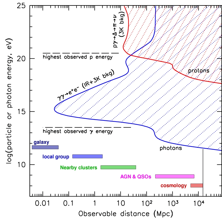
Above ∼ 1 TeV, photons traveling >100 Mpc are attenuated by infrared background radiation (figure

1.4). The density of the infrared background is not well known, therefore the absolute luminosities

of distant TeV photon sources are uncertain. Above 100 TeV, pair production on the much more

numerous CMB photons limits photon range to ∼ 1 Mpc, and above 1 PeV, only our galaxy is visible.

Figure 1.4: Observable distance for photons and protons, from P. Gorham [65].

1.2.3 Neutrinos

The interaction of Neutrinos with matter is described in detail in chapter 2. The universe is

essentially transparent to neutrinos at energies up to ∼ ZeV; therefore neutrinos can travel unimpeded

from cosmological distances. The transparency of matter to neutrinos presents an obvious problem

for neutrino detection, discussed in chapter 2.

1.3 Cosmic Ray Air Showers

Charged particles and photons interact upon entering the upper levels of the relatively dense

atmosphere and initiate air shower cascades. Air showers initiated by photons and electrons prop-

agate electromagnetically and differ considerably from those initiated by hadrons, which proceed

additionally by the strong nuclear force.

1.3.1 Electromagnetic Showers

Electrons and positrons with energies above ∼ 100 MeV primarily lose energy via bremsstralung

and emit high energy photons. Photons at such energies dominantly produce electron-positron pairs

on the nuclear or electron fields. The radiation length for either process in the air is λ

∼ λ

∼ 40

g/cm

; the resulting cycle between photons and electrons/positrons results in a smooth, geometric

increase of photons and electrons with depth up to a shower maximum, where the increase is over-

taken by particle losses from the shower. The maximum occurs deeper in the atmosphere at higher

energies. Finally, photons occasionally produce muon-antimuon pairs. The energy loss rate of muons

is much less than electrons of similar energy (section 2.2), and these muons can carry shower energy

significantly deeper than the electrons and photons.

1.3.2 Hadronic Showers

Cosmic ray protons and nuclei initiate hadronic showers in the atmosphere and produce pions,

kaons, and heavier mesons, illustrated in figure 1.5. These mesons receive a fraction of the primary

energy and therefore follow the primary cosmic ray spectrum of ∼ E

? 2 . 7

. Hadronic interaction lengths

are somewhat longer than electrons and photons, with λ

∼ 80 g/cm

for nucleons and λ

∼ 120 g/cm

for pions. Charged pions and kaons alternatively can decay and produce muons and neutrinos,

Decay

Hadronic

shower

Cosmic

ray

Electromagnetic

shower

→

Figure 1.5: Illustration of a cosmic ray air shower, from [66].

100

− 9

− 10

− 8

− 7

− 6

− 5

− 4

− 3

− 2

Vertical intensity (m

−

)

Depth [km water equivalent]

Figure 1.6: Muon flux vs. depth, from [2]. Muons induced by atmospheric neutrinos

are relatively constant with depth and dominate the muon flux for depths greater than

20 km water equivalent.

described in the next section. The mesons carry energy away from the core of the shower, making

the energy density within hadronic showers considerably more uneven than within electromagnetic

showers. Finally, hadronic showers are generally accompanied by an electromagnetic component

initiated by photons from the relatively instantaneous decay of charged pions.

1.3.2.1 Atmospheric Muons and Neutrinos

Mesons produced in hadronic showers may decay before interacting, producing muons and

neutrinos which carry energy well beyond the maximum extent of the electromagnetic component of

the shower and penetrate deep into the Earth. Measurements of the cosmic ray muon flux as a function

of depth are shown in figure 1.6. The probability of meson decay is suppressed by the Lorentz factor,

and the suppression is asymptotically E

? 1

at high energies. For atmospheric neutrinos, this results

/ GeV

log

1.5

2.5

3.5

-1

-2

/dE / GeV

log

-1.8

-1.7

-1.6

-1.5

-1.4

-1.3

-1.2

AMANDA-II (2000-2006, 90% CL)

GGMR 2006

Barr et al.

Honda et al.

Figure 1.7: Measured and predicted atmospheric neutrino flux vs. energy, from [67].

in an energy spectrum of ∼ E

? 3 . 7

above ∼ TeV. Measurements [67, 68] and models [69, 70] of this

atmospheric neutrino flux are shown in figure 1.7. The meson interaction probability strongly depends

on gas density, with low density favoring decay; thus, the atmospheric neutrino and muon rates vary

seasonally, with higher rates produced by the less dense summer atmosphere, and at shorter time

scales according to the stratospheric weather in the top 20 kPa of the atmosphere. Mesons entering

the atmosphere at slanted angles also encounter less atmospheric mass, favoring decay; therefore, the

atmospheric neutrino flux is zenith-dependent. Heavy mesons, including charm mesons, decay before

interaction and should yield an additional ∼ E

? 2 . 7

component to the atmospheric neutrino and muon

spectra. These prompt neutrinos should increase the atmospheric neutrino flux at high energies, but

prompt fluxes have not yet been observed [26] and prompt models (e.g. [71]) are largely uncertain.

1.4 High Energy Astronomy

An ultimate goal of cosmic ray physics is astronomy, tracing high energy particles back to their

origins and thus correlating cosmic ray emission with known astrophysical objects, perhaps some of

the candidates described in section 1.1.3. TeV photon astronomy has been very successful; however,

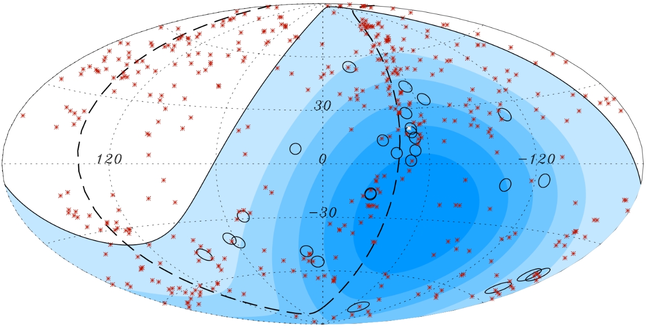
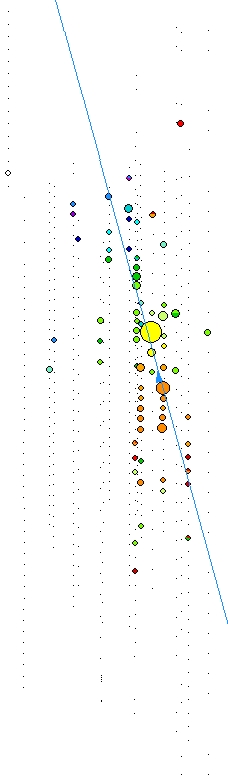
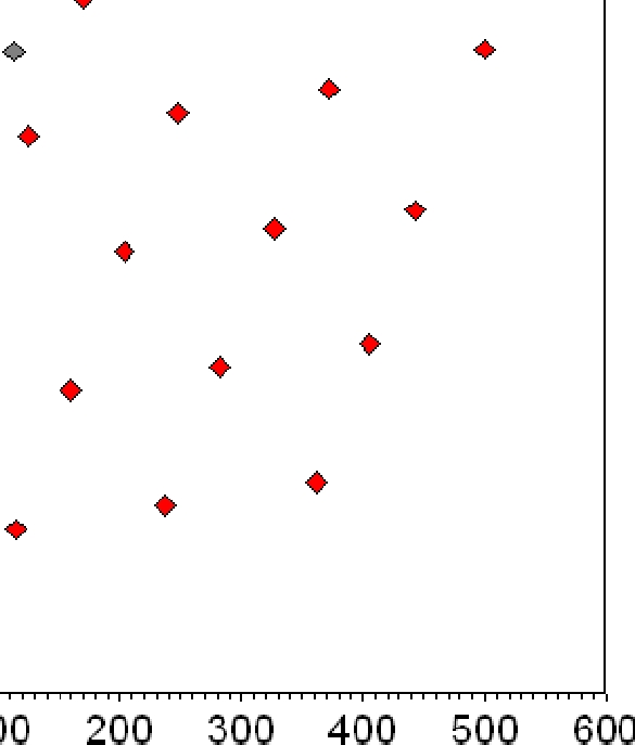
Figure 1.8: Skymap of 27 UHE cosmic ray events observed by Auger [73] with 3.1

◦

angular ellipses (black) and AGN within 75 Mpc (red asterisks).

there is no strong evidence linking hadronic cosmic rays, which constitute the bulk of the cosmic ray

flux, with any particular sources.

1.4.1 Charged Particles

Charged particles are deflected by magnetic fields, effectively scrambling their trajectories

through galactic and intergalactic space. Magnetic effects are minimized by selecting only the highest

energy cosmic ray events, which have the largest gyroradii, at a cost of reducing the data to a handful

of events above a few tens of EeV. The AGASA and Auger air shower arrays reconstruct these high

energy events with ∼ 1

◦

– 1.5

◦

angular resolution, while the Auger and HiRes fluorescence detectors

are more accurate. No significant excesses at any point in the sky consistent with the detector

angular resolution have been observed by AGASA and HiRes [72]. If no individual source produces

a significant excess, the cumulative excess from a catalog of potential sources may still be significant.

Such source stacking approaches may detect this cumulative excess and are further described in

section 7.2.4. Auger reports a marginally significant correlation of 27 recorded cosmic ray events

with energies above ∼ 60 EeV, shown in figure 1.8, to a catalog of AGN within 75 Mpc [73]. A similar

correlation is not observed by HiRes [74] using the same source catalog.

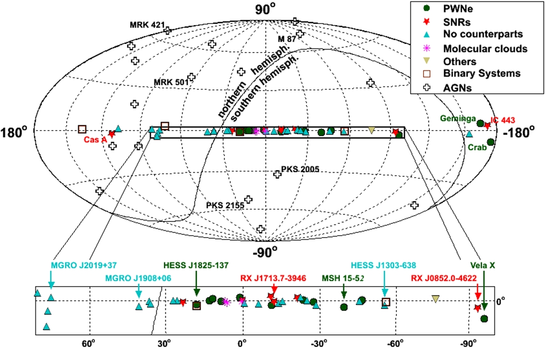
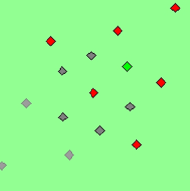
Figure 1.9: Known TeV gamma ray sources listed according to known astrophysical

counterparts, courtesy of A. Kappes.

1.4.2 Photons

Gamma ray astronomy has now discovered 75 sources with TeV photon emission [46], many

of them shown in figure 1.9. The extragalactic TeV sources discovered to date generally have AGN

counterparts. Most galactic TeV sources are associated with supernova remnants and microquasars,

although some do not have identified counterparts.

TeV photon experiments are broadly classified into two types: Imaging air-Cherenkov tele-

scopes (IACTs) and high-density air shower arrays. The newest IACTs [75, 76, 77] image the

Cherenkov light produced by atmospheric air showers (section 2.3.1) onto a “camera” array of photo-

multiplier tubes using a large diameter ( ∼ 12 – 17 m) mirror array. Reconstruction of the air shower

uses camera timing and pixel position information, and is accurate to ∼ 0.1

◦

. IACTs have a field of

view of ∼ 3

◦

– 5

◦

and operate only on clear, moonless nights. Alternatively, air shower gamma ray

experiments [78, 79, 80] record the electromagnetic shower directly, and reconstruction of the shower

front gives ∼ 1

◦

pointing resolution. Air shower experiments are largely complimentary to IACTs.

IACTs have significantly better pointing resolution and a lower energy threshold; however air shower

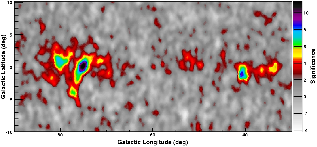
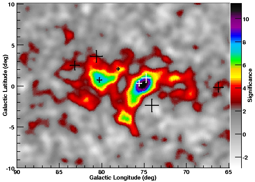
Figure 1.10: Milagro skymap showing TeV gamma ray sources near the galactic plane,

with several strong sources in the Cygnus region [81].

experiments observe nearly half the sky simultaneously and are capable of an almost 100% duty cycle.

From the perspective of potential hadronic cosmic ray acceleration, the sources with the highest

energy photon emission are some of the most interesting. Several new TeV sources [18], shown in

figure 1.10, discovered by the Milagro air shower array are particularly compelling. The sources are

galactic, and a cluster of activity exists near the Cygnus region. Several of the sources have been

subsequently observed by IACTs [82, 83] and exhibit hard power law spectra with γ ∼ 2, indicative

of Fermi acceleration. The energy spectrum observed by HESS for the source MGRO J1908+06 is

shown in figure 1.11. An observation of high energy neutrinos from MGRO J1908+06 and other TeV

photon sources would confirm a component of the TeV emission is from pion decay and establish the

sources as regions of cosmic ray acceleration.

)

-1

TeV

-1

sec

-2

dN/dE (cm

-17

-16

-15

-14

-13

-12

-11

-10

-9

PRELIMINARY

MILAGRO

HESS

3.23

0.45

-1

TeV

-1

-2

-12

x 10

= 2.08

0.10

Energy (TeV)

-1

Residuals

-1

Figure 1.11: Energy spectrum of MGRO J1908+06 measured by HESS [82].

Chapter 2

High Energy Astronomy with Neutrinos

High energy (>TeV) neutrino astronomy is a long standing goal of astrophysics. Since neutri-

nos are neither deflected by magnetic fields nor significantly attenuated by matter and radiation en

route to Earth, neutrino astronomy offers an undistorted view of the high energy universe. Particu-

larly, since high energy neutrinos are an end product of high energy hadronic processes and are not

produced by electromagnetic processes, neutrino astronomy offers an opportunity to unambiguously

identify the sources of cosmic rays.

Neutrinos interact with matter through the weak nuclear force and thus have much smaller

interaction cross sections than photons or charged particles; neutrinos can pass through a significant

portion of the Earth. These small cross sections present the most significant difficulty associated with

neutrino detection. Very large detectors are necessary to record enough neutrino interaction events

to observe the predicted small neutrino fluxes.

2.1 Neutrino Interaction

Four neutrino interaction modes are generally considered:

+X →?

+ X

(Neutral Current)

+X →?

l + X

(Charged Current)

ν¯

+ e

→?

(Glashow Resonance)

+ ν¯

→?

(Z-Burst)

where l is the neutrino flavor eigenstate, electron (ν

), muon (ν

), or tau (ν

). The cross sections of

the first three of these modes are shown in figure 2.1. These modes involve the following processes.

• Neutral Current : The neutrino exchanges a Z boson with a nucleon, depositing a fraction of

its energy and initiating a hadronic cascade. The original neutrino exits the interaction with

reduced energy and an angular deviation.

• Charged Current : The neutrino exchanges a W boson with a nucleon, initiating a similar

hadronic cascade. Additionally, an energetic lepton is produced with a substantial fraction of

the initial neutrino energy.

• Glashow Resonance : For the interaction of anti-electron neutrinos with electrons, resonant

production of W bosons occurs at neutrino energies near ∼ 6.3 PeV and significantly enhances

the anti-electron neutrino cross section, shown in figure 2.1. Equivalent interactions are possible

with muon and tau flavors, but neither muons nor tau particles are currently practical targets.

• Z-Burst : Resonant production of Z bosons is possible for interactions between antineutrinos

and neutrinos at an energy E ∼

4E’

if the target neutrino is relativistic with energy E’

or E =

2 m

if the target neutrino is nonrelativistic. One particular target is the theorized

cosmologic neutrino background, which would partially absorb UHE neutrinos [85] above ∼ 10

eV. Z-bursts, however, do not provide a practical way to detect high energy neutrino fluxes at

Earth.

Neutral current and charged current interactions provide the potential to detect neutrinos over a

significant energy range, with the associated cross sections increasing with neutrino energy, and anti-

electron neutrino detection is enhanced near the ∼ 6.3 PeV Glashow resonance. All three modes

produce cascades which can be detected when the interaction occurs within the detector volume.

Additionally, charged current interaction produces charged leptons, and electrons, muons, and tau

particles have characteristic energy loss signatures.

2.2 Lepton Propagation

The pattern of energy deposition along the lepton path is determined by the relative rate of

continuous losses from ionization, large stochastic losses from bremsstralung, pair production, and

photonuclear interactions, and for muons and especially tau particles, lepton decay.

[

GeV

]

[

]

-38

-37

-36

-35

-34

-33

-32

-31

-30

Figure 2.1: Neutrino cross sections for charged current (blue) and neutral current (red)

for ν (solid) and ν¯ (dashed), from [84]. Also shown is ν¯

+ e

→?

(dotted green)

with the Glashow resonance at E

∼ 6.3 PeV.

ioniz

brems

photo

epair

decay

energy

[GeV]

energy losses

[

GeV/(g/cm

)

]

-10

-9

-8

-7

-6

-5

-4

-3

-2

-1

1 10 10

Figure 2.2: Muon energy losses in ice, from [84].

2.2.1 Electrons

Electron energy losses are strongly dominated by bremsstralung above ∼ 1 GeV in ice and

other materials. Electrons deposit all of their energy within a few meters water equivalent (mwe),

leaving relatively short and bright electromagnetic cascades.

2.2.2 Muons

Muon energy losses in ice are shown in figure 2.2 as a function of muon energy. Loss rates

are generally much smaller than those of electrons at the same energy due to the significantly larger

relative mass of the muon; therefore muons produce significantly longer tracks. Below ∼ 1 TeV, con-

tinuous energy losses from ionization dominate, with losses of 200 MeV per mwe. Above ∼ 1 TeV,

stochastic losses become significant and substantially increase the energy loss rate, rising proportion-

ally with the muon energy. The typical muon track length is roughly proportional to energy up to

∼ 1 TeV, reaching ∼ 2.5 km. Above ∼ 1 TeV, the muon track length increases logarithmically with

energy, reaching ∼ 20 km at 1 PeV [84]. Thus, muons do not need to interact within the detector to

be observed; they propagate from significant distances.

2.2.3 Tau Particles

Tau particles produce short tracks ending in decay due to the short tau lifetime of ∼ 3 × 10

? 13

s. At the decay vertex, a tau neutrino is regenerated and a cascade is produced for hadronic and

electron decay modes. This “double bang” signature, with a cascade at the start and end of the

track, is unique to tau events. The two cascades are separated by a short track length, determined

by the tau Lorenz factor, of ∼ 100 m for tau energies of a few PeV. The secondary tau neutrino, with

a fraction of the primary neutrino energy, propagates from the vertex and may interact again. The

tau track itself is not as energetic as a muon track due to the higher relative mass of the tau. Finally,

tau decay produces a muon rather than a cascade with a branching ratio of 17.4%.

2.3 TeV Neutrino Detection

The most sensitive method currently available for TeV neutrino detection is the optical Cherenkov

technique. Water and ice serve as practical Cherenkov radiative media, as they have good optical

properties and are available in large volumes. An array of optical sensors is placed in the water or

ice, and the Cherenkov light produced by tracks and cascades within the detector active volume are

recorded as events. Energy resolution and angular resolution are critical to distinguish astrophysical

neutrino events from the background of muons and neutrinos from cosmic ray air showers.

2.3.1 Cherenkov Radiation

Cherenkov radiation is emitted by transparent, electrically insulating media when relativistic

charged particles pass through, provided the particle velocity is greater than the phase velocity of

light in the medium at a given wavelength. The photons propagate from the track in a conical shock

front, emitted at an angle

cosθ

βn

(2.1)

relative to the track, where β =

and n

is the group index of refraction of the medium. For

relativistic leptons with energies above 10 GeV, β ∼ 1. The Cherenkov angle θ

is 1.4

◦

in air for

visible wavelengths and 100 kPa, and θ

is 40.5

◦

–42.5

◦

in water or ice, depending on the wavelength.

(nm)

400

450

500

550

600

)

−1

(cm

N/dxd

0.6

0.8

1.2

1.4

Figure 2.3: Cherenkov wavelength distribution in ice, using the index of refraction

parametrization of [86].

The wavelength distribution of Cherenkov photons is given by the Franck-Tamm formula,

dxdλ

2πα

1 ?

(λ)

(2.2)

and is weighted toward shorter wavelengths, as shown in figure 2.3. The number of expected

Cherenkov photons per unit track length is found by integrating the Franck-Tamm formula over

the wavelength band of interest. This number is roughly 210 photons per centimeter in ice for the

wavelength band 365 nm – 600 nm, with the upper wavelength bound imposed by ice transparency

[87], and a practical lower bound of 365 nm due to the ultraviolet absorption of glass used to house

the photon counting apparatus [88].

2.3.2 Energy Resolution Considerations

An event energy estimate is possible by measuring the amount of Cherenkov light in the

detector, as more energetic events produce more secondary particles and more Cherenkov light. For

electron neutrino cascades, all secondary particles are produced a short distance from the interaction

vertex. When such events are fully contained within the detector, good energy resolution is possible.

Energy estimation is also possible for muons, as energetic muons emit more light during stochastic

energy losses, which appear as cascades along the muon track. In [84], the muon energy loss is

parametrized as

= a + bE,

(2.3)

with a ∼ 0.268 GeV/mwe (ionization) and b ∼ 4.7 × 10

? 4

/mwe (stochastic) for ice. Below ∼ 1 TeV,

ionization losses dominate, making energy estimation extremely difficult. Two additional factors com-

plicate energy measurement with muons: First, the muon stochasticity limits the energy resolution.

The number and intensity of stochastic losses within the detector volume is random and variable.

Finally, the muon energy estimate is not strongly correlated to the primary neutrino energy, which

is the interesting quantity. The distance any muon travels to the detector is generally unknown, and

energy losses en route make the muon energy estimate a lower limit of the primary neutrino energy.

2.3.3 Angular Resolution Considerations

Angular reconstruction is possible using the space-time pattern of Cherenkov light recorded

by the array of optical sensors. Electron neutrino cascades are generally contained within a few

mwe, which is very short compared to the dimensions necessary for a large detector. Although these

cascades are asymmetric, they appear rather spherical due to photon scattering, and therefore the

direction of the primary neutrino is reconstructed poorly. In contrast, TeV muons typically pass

through the detector, creating tracks with a large lever arm for accurate reconstruction. The muon

track is offset from the primary neutrino track by a median angular deviation parametrized [89] by

∆ψ = 0.7

◦

TeV

? 0 . 7

(2.4)

Long tau particle tracks and double bangs should also have good angular resolution. For neutrino

astronomy, angular resolution is essential; therefore, this work focuses only on track-like events.

2.4 The Earth as a Neutrino Target

Neutrinos must interact near the detector to be observed. Upgoing neutrinos must pass through

nearly the full diameter of Earth to reach the detector, while downgoing particles need only traverse

the detector overburden, generally a few thousand mwe. The column depth a particle must travel

through the Earth to a detector 1500 mwe below the surface of Earth is shown in figure 2.4. For the

vertical upgoing direction (cos θ ∼ –1), the column depth through the Earth is sufficient to attenuate

neutrinos above ∼ 100 TeV. The precise column density for near-vertical neutrinos penetrating the

inner core of the Earth is uncertain due to uncertainties in the inner core density and radius. Attenua-

tion measurements of upgoing neutrinos above ∼ 10 TeV are expected to constrain these uncertainties

[91]. The column density decreases as zenith angle becomes more horizontal, such that ∼ PeV neutri-

nos penetrate to the detector at cosθ ∼ –0.4, and EeV neutrinos are visible above cosθ ∼ –0.05. Tau

neutrinos are an exception, as secondary neutrinos produced by tau decay may still propagate to the

detector, allowing observation of PeV – EeV tau neutrinos from steeply upgoing zenith angles. For

downgoing zenith angles cosθ > 0.05, the column depth becomes less than maximal muon ranges.

Since neutrino-induced muon fluxes increase from the surface until an equilibrium is reached between

muons ranging out and charged-current muon neutrino interactions producing muons, downgoing

zenith angles may not have sufficient column depth to reach this equilibrium and subsequently have

smaller neutrino-induced muon fluxes. Additionally, muons from cosmic ray air showers are able to

reach the detector at downgoing zenith angles.

2.5 The Background from Cosmic Ray Air Showers

Downgoing muons from cosmic ray air showers penetrate to the detector for cosθ > 0.05 and

dominate muons from neutrino charged current interactions, increasing the background of track-like

events by several orders of magnitude. This background limits sensitivity to neutrino-induced muon

tracks to the upgoing zenith range cosθ < 0.05. Two techniques are under development to extend

sensitivity to cosθ > 0.05. The first uses energy cuts and searches for ∼ PeV neutrinos [92], since

the cosmic ray muon background is much smaller at those energies. Another technique searches

for neutrino-induced muons starting within the detector, rejecting the cosmic ray muon background

passing completely through, and should be sensitive at ∼ TeV neutrino energies. The remaining

chapters focus on neutrino astronomy for only the upgoing region cos θ < 0.05.

While the zenith range cosθ < 0.05 is free from cosmic ray muons, the neutrinos from cosmic

ray air showers easily penetrate to the detector. This atmospheric neutrino background presents the

greatest challenge to TeV neutrino astronomy in the upgoing zenith range. Astrophysical sources can

be distinguished from this background by searching for spatial excesses comparable to the detector

resolution. Additionally, astrophysical neutrino sources with energy spectra ∼ E

? 2

would produce

Column Depth (mwe)

−1

cos

−1 −0.8 −0.6 −0.4 −0.2 0

0.2 0.4 0.6 0.8

Cosmic Ray Muons + Neutrinos

Neutrinos

=10 TeV

=1 PeV

=1 EeV

=1 PeV

Cosmic Ray Muon

Dominated

Neutrino Dominated

Detector

z = −1500 mwe

EeV

PeV

TeV

Figure 2.4: Column penetration for muons and neutrinos as a function of zenith angle

for a detector 1500 mwe below the surface. Earth column density is calculated from

the Preliminary Reference Earth Model [90].

excesses at high energy relative to ∼ E

? 3 . 7

atmospheric neutrinos. The method used to identify these

excesses is described in chapter 6 and represents a significant portion of this work. Many sources are

additionally expected to exhibit time-dependent fluxes. Such time dependence provides additional

power to identify these sources, and methods including time dependence are described in appendix B.

Chapter 3

The AMANDA Cherenkov Telescope

The Antarctic Muon And Neutrino Detector Array (AMANDA) is a large optical Cherenkov

detector built in the ice sheet at the geographic South Pole. AMANDA has been designed with the

intent of observing high energy astrophysical neutrinos, or at minimum proving the concept of in-ice

optical Cherenkov detection and paving the way for a larger detector.

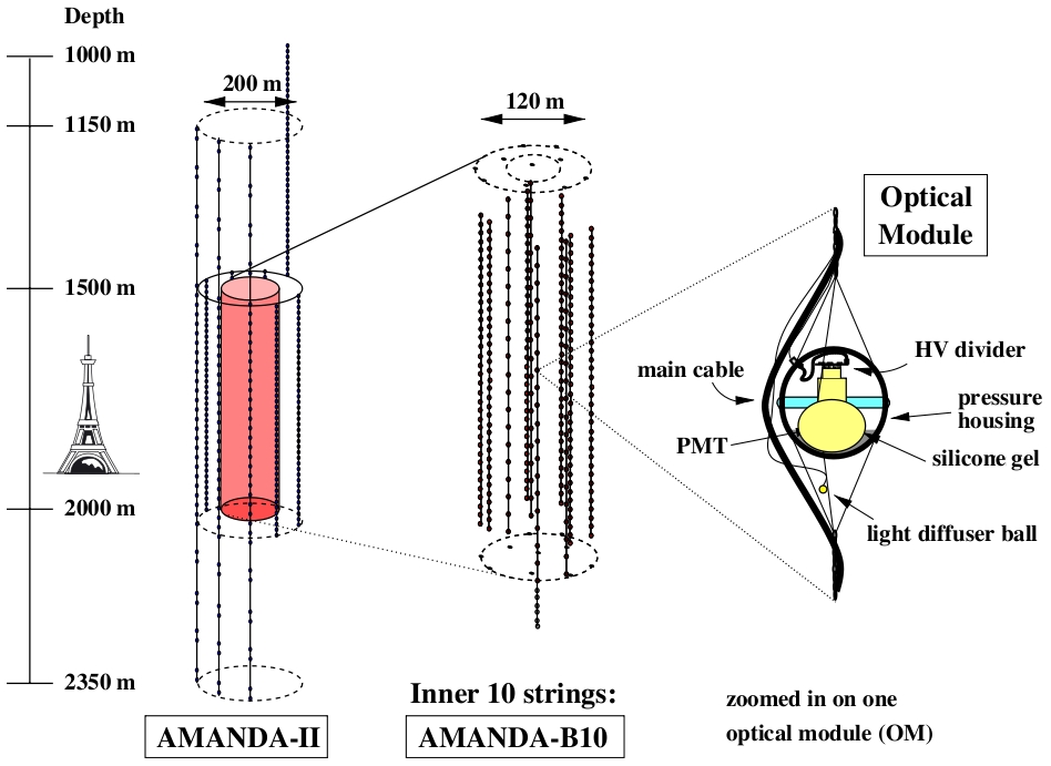
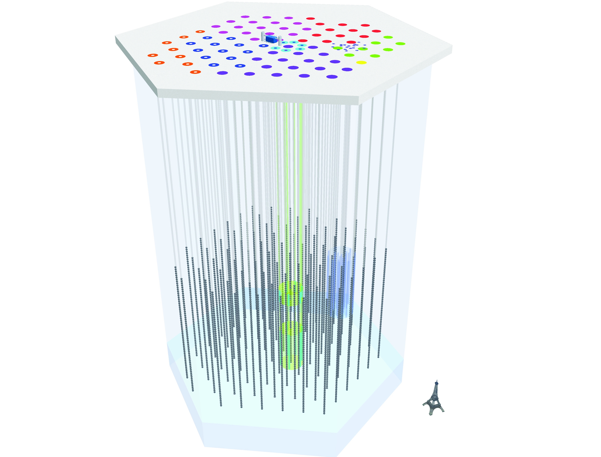
3.1 In-Ice Array

The main component of AMANDA is an array of photosensitive modules frozen beneath the

ice sheet. The array (figure 3.1) consists of 677 optical modules arranged in 19 vertical strings, which

roughly form a vertical cylinder of 200 m diameter. Most optical modules lie in the region from 1500

m to 2000 m below the ice surface.

Installation of each string consists of first drilling a hole through the firn, roughly the first 50

m, with a closed circulation of hot ( ∼ 90

◦

C) water. Drilling of the underlying ice then commences

with an open circulation of hot water, possible because the ice, unlike the firn, retains the water well

created. The string of optical modules is lowered into the water when drilling is complete, with each

module installed in-turn on the main cable as it descends. The strings freeze into place within a few

days. A significant fraction of modules ( ∼ 7%) do not survive installation/refreeze and are lost. The

inner ten strings, dubbed AMANDA-B10, were installed by early 1997. The AMANDA-II detector

was completed by early 2000 with nine final strings.

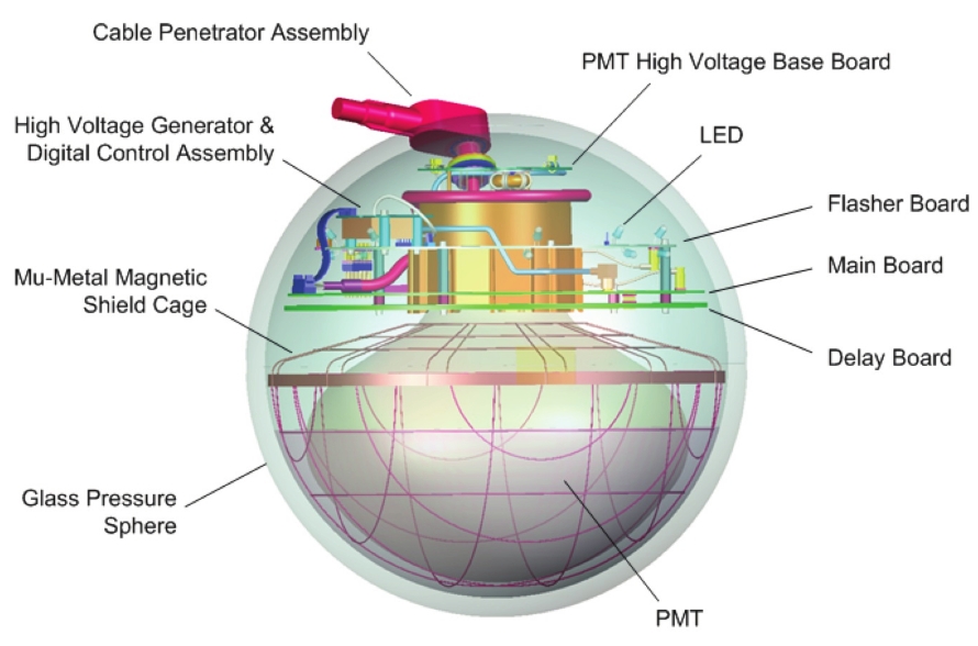
Each string contains roughly 40 optical modules. The main component in each module is an 8

inch Hamamatsu R5912-2 photomultiplier tube (PMT) with a bialkali photocathode, which performs

Figure 3.1: The AMANDA-II in-ice array and optical module, from [93].

with ∼ 20% quantum efficiency and a timing resolution of <5 ns. The PMT is optically coupled to a

30 cm glass pressure sphere housing using silicone gel. The main cable provides high voltage to each

module, divided by internal circuitry and providing the appropriate voltage to each PMT dynode.

Each module has an individual set voltage, and the voltages are tuned to provide a gain of ∼ 10

for all modules in the array. The main cable also provides analog transmission of PMT signals to

the surface via coax, twisted pair, and analog-optical channels. String-18 [94], unlike the remainder

of the array, has remote data acquisition electronics in each module and communicates digitally to

the surface. This string was designed as a prototype for IceCube [95] optical modules and data

transmission.

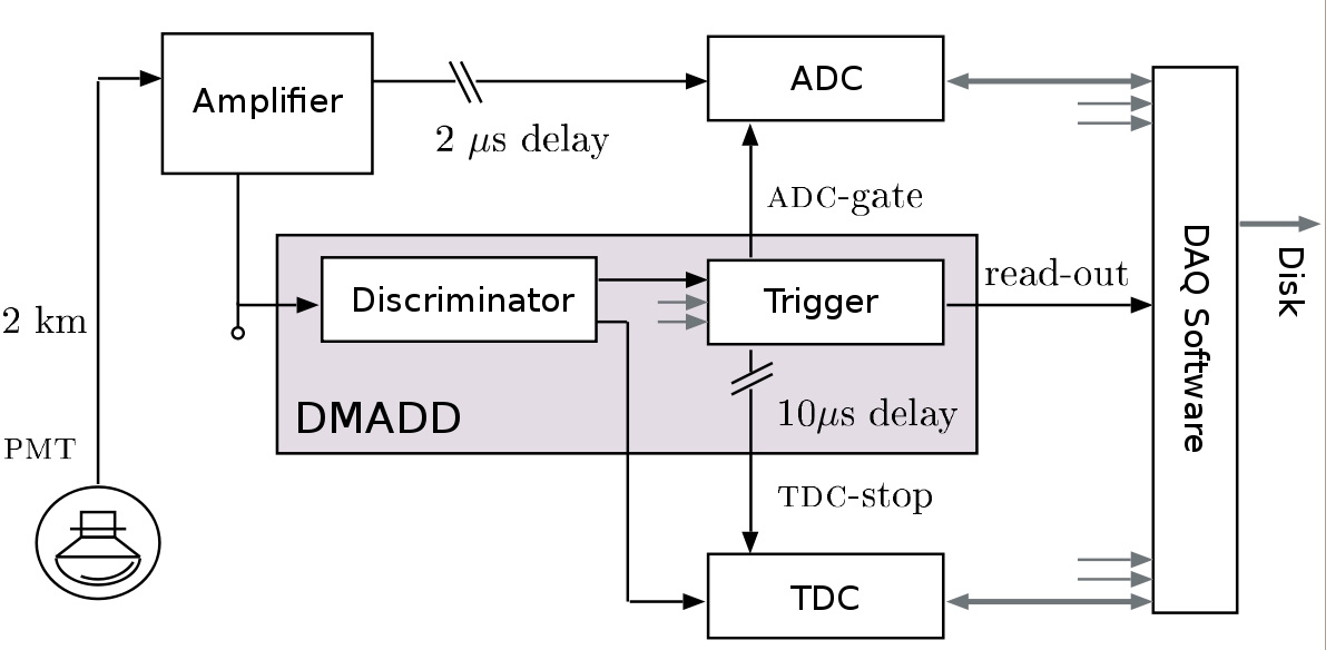
3.2 Muon-DAQ

The AMANDA muon-DAQ system is illustrated in figure 3.2. PMT pulses from electrical

channels are first amplified, then fed to a discriminator. The pulse is also sent to a peak-sensing

ADC through a 2 µs delay. Pulses in analog-optical channels are converted to electrical and are

routed similarly to discriminators and ADCs. For all channels, the discriminator fires when the

channel pulse amplitude exceeds the discriminator threshold (a “hit”), and the discriminator output

signal is fed to a TDC and the trigger. The vast majority of hits are optical noise, produced by

K decay in the glass PMT face and pressure sphere. The trigger logic, the main component of

the DMADD (Digital Multiplicity ADder-Discriminator) module, provides triggers according to the

following specifications:

• 24-fold multiplicity trigger, when 24 modules register hits within 2.5 µs.

• String trigger, requiring a set multiplicity from the same string. This trigger, designed to retain

low multiplicity events and thus low energy muons, requires hits in 6 modules from inner strings

1-4 or hits in 7 modules from strings 5-19 within 2.5 µs.

When the trigger fires, a digitization signal is sent to the bank of ADCs, which digitize the pulse

peak amplitudes. A stop signal is sent to the TDC bank through a 10 µs delay. Each TDC records

the times of both positive and negative edges for a maximum of eight successive threshold crossings,

and the time over threshold (TOT) for each pulse can be calculated. The ADC and TDC banks are

Figure 3.2: Schematic of the AMANDA muon-DAQ, adapted from [97].

read out along with the trigger. The hit and trigger times are calibrated to GMT time and stored on

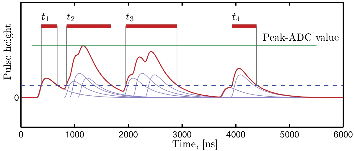
disk. The process of triggering, reading, and clearing the DAQ components requires ∼ 2 ms, during

which the detector cannot record another event. An illustration of the data obtained is shown in

figure 3.3. A more advanced data acquisition system was installed in early 2003 [96], providing full

PMT waveforms and operation without deadtime; however, data from this system is not discussed

further.

3.3 Calibration

An accurate understanding of detector relative timing and geometry are critical since muon

reconstruction is based on these quantities. Each channel has a specific cable and electronics propa-

gation time delay. These delays are measured by injecting light at known times with a surface laser

through an optical fiber, which has a known optical propagation delay, to modules in the array. The

calibration is of the form

t = t

raw

? T

√

(3.1)

Figure 3.3: Illustration of the data available from the AMANDA muon-DAQ, from

[97]. For each hit module, we record the overall peak ADC value and the times of

positive and negative edges for up to eight discriminator crossings. The red curve

represents the sum of several individual PMT pulses.

where T

is the main correction factor and α/

√

A is an amplitude-dependent factor necessary due to

pulse distortion. Systematic uncertainty in the calibration adds to the PMT jitter and results in ∼ 15

ns end-to-end timing uncertainty. Accurate surveys of (x,y) coordinates for each string are recorded

during deployment. The z position of each module on the string is determined by a combination of

the known position along the main cable and the depth of the bottom of the string, determined by

pressure readings at the end of deployment. These measurements are improved using laser pulses,

since the distance of a module to a light source is known:

d = (t

rcv

? t

emit

) ×

ice

(3.2)

where t

rcv

and t

emit

are the reception and emission times of the light pulse, respectively, and n

ice

the group index of refraction of South Pole ice.

3.4 Properties of South Pole Ice

Cherenkov photons produced by relativistic leptons propagate through ice before reaching

optical modules. The photons propagate at a velocity c/n

, where n

is the group index of refraction,

which varies from 1.38 at 337 nm to 1.33 at 532 nm [86]. The ice within the detector volume is

composed of two general categories: Undisturbed glacial ice and hole ice.

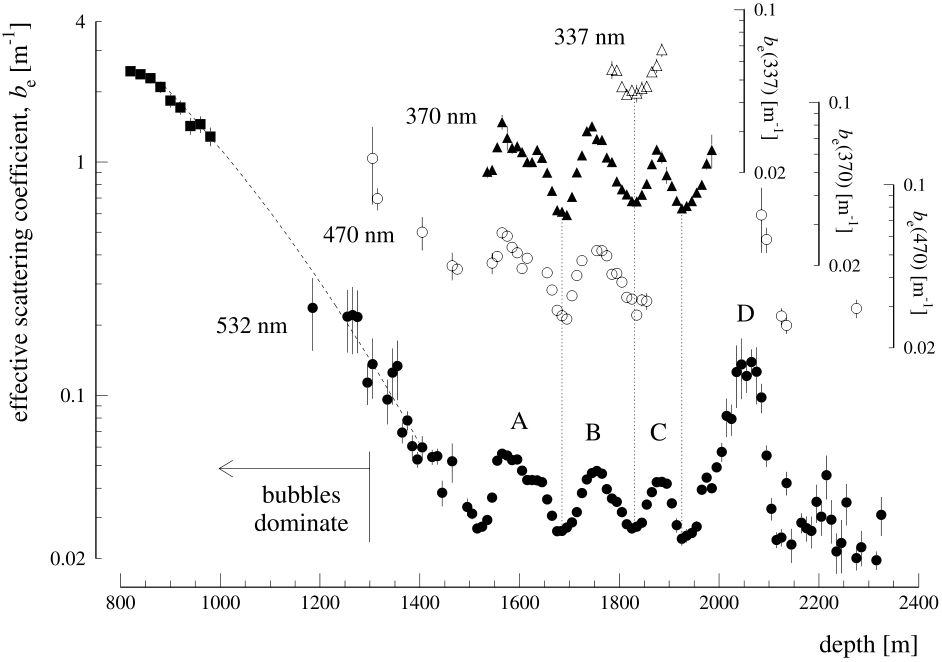
3.4.1 Glacial Ice at the South Pole

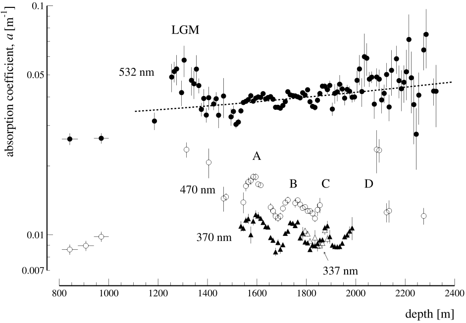
Measurements show that the glacial ice at the South Pole is distinctly layered, with nearly

an order of magnitude variation in scattering and absorption coefficient as a function of depth [87],

shown in figure 3.4. This depth dependence is due to the time-variable accumulation of dust onto the

glacier surface, sinking deeper into the glacier with time as more snows accumulate. High resolution

studies of this ice [98] reveal individual explosive volcanic events. Above 1400 m, scattering from

bubbles within the ice becomes increasingly significant, rendering this region less useful for Cherenkov

detection. Below 1400 m, time and pressure have transformed these bubbles into air hydrate crystals,

making the ice significantly more transparent.

3.4.2 Hole Ice

As water refreezes within holes after string deployment, the ice formed is significantly different

from the bulk of the ice. Scattering and absorption are constant with depth due to mixing. More

importantly, refreezing forces air out of the water, forming bubbles and significantly increasing scat-

tering. The effective scattering coefficient for hole ice is not well-measured, but may be 50 cm or

less.

3.5 Simulation

An accurate simulation of AMANDA is required to understand the detector response to muon

and neutrino fluxes over a wide energy range, thereby quantifying the event expectations of meaningful

neutrino signal hypotheses. We simulate fluxes of muon and tau neutrinos with ANIS [99], using the

CTEQ5 [100] structure functions and Preliminary Reference Earth Model [90]. Muons produced by

ANIS are propagated with MMC [84], which simulates muon decay and stochastic losses.

Figure 3.4: Scattering coefficient (top) and absorption coefficient (bottom) of South

Pole ice as a function of depth (from [87]), showing scattering/absorption peaks A-D.

Cherenkov light produced by muons and cascades near the detector is simulated by PTD.

Using a photon Monte Carlo, photon densities are tabulated in terms of radial distance from the

muon track (or cascade axis), z distance along the axis, time, and PMT orientation. The simulation

does not account for depth-dependent ice properties, and instead assumes the following scattering

properties of the bulk ice, obtained by matching event rate and timing distributions with downgoing

muon tracks:

eff

scat

= 21 m

< cosθ

scat

> = 0.85

Absorption is modeled with wavelength dependence, with a typical absorption length of λ

= ∼ 100 m.

Hole ice is simulated with a scattering length of λ

eff

scat

= 50 cm. Photonics [101], a newer ice simulation

which includes layering, is now used. The detector simulation AMASIM [102] uses these photon

density tables; photon hits in optical modules and the hit timing are determined by Monte Carlo.

For tracks with multiple muons or muons with stochastic losses and resulting cascades within the

detector, photon densities are summed appropriately. Cosmic ray air showers are also simulated

using CORSIKA [103], and resulting muons are propagated through the same simulation chain using

MMC and AMASIM.

Chapter 4

Data Selection and Event Reconstruction

4.1 Data Selection

The raw AMANDA muon-DAQ data returned from the South Pole are mostly downgoing

muons from cosmic ray air showers, which are recorded at a rate of ∼ 80 Hz, with only a few neutrino-

induced muon events per day. The data is filled with problematic periods corresponding to hardware

glitches, including power outages, HV failures, DAQ failures, etc. Similarly, a large fraction of the

optical modules experience transient problems or are simply dead. Such unstable time periods and

optical modules reduce our ability to properly simulate the detector and assess livetime, both of

which are critical to evaluate the detector response to a simulated neutrino flux, so this bad data

must be removed. The most sensitive stability indicator is the individual dark noise rates of all optical

modules. This noise rate is measured for each module by counting hits from triggered events which

occur well before the trigger time, and thus are not likely to have been produced by the event causing

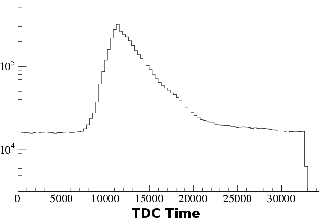
the trigger. For 2005 and 2006, a reasonable time window is ∼ 0 – 7000 ns (TDC < 7000), shown in

figure 4.1. The number of total hits within this time window for typical 10 minute AMANDA runs

should follow a Poisson distribution, and the noise rate for each optical module (OM) is given by

R =

hit

trig

· 7 µs

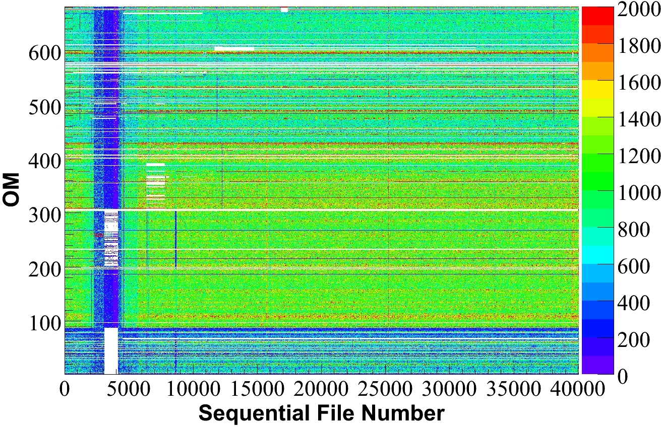
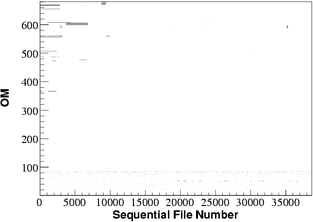
. Obvious non-Poissonian structure is visible in a 2-D noise rate histogram of OM vs.

time for 2005, shown in figure 4.2.

For 2000-2004, stability cuts have been developed to remove unstable periods, using the number

of OMs outside of a noise rate range 83 Hz < R < 8.3 kHz as a stability indicator. OMs have been

removed using cuts on both the number of files with noise rates outside the above range and the

Figure 4.1: TDC time distribution of hits for triggered events during AMANDA run

9363 in 2005. One TDC unit is ∼ 1 ns. The peak near 11,000 is comprised mostly of

hits from muons.

Figure 4.2: 2005 Noise rate matrix of OM vs. sequential raw data file.

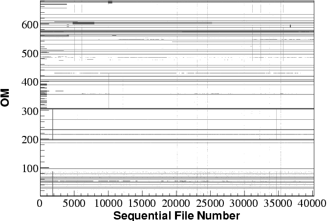
Figure 4.3: Matrix of 2005 data quality before (left) and after (right) quality cuts are

applied. Black regions indicate noise rates below 83 Hz or above 8.3 kHz.

RMS fluctuation of the noise rate [104]. However, since problematic files and problematic OMs are

correlated, a better way to do the filtering is to remove the most unstable OM or file and recompute

the stability of the remaining OMs and files, then repeat the process until the data shows acceptable

stability. This procedure has been performed on the 2005 and 2006 AMANDA data using a log-

likelihood approach, using the following parameters as a measure of stability:

= ?

?OM

i =1

log[P( R| < R >)]

(4.1)

= ?

i =1

log[P( R| < R >)],

(4.2)

where Q

and Q

are the file and OM quality, N

is the number of remaining optical modules,

is the number of remaining files, and < R > is the mean noise rate for the given OM. The OM

or file with the highest value of Q is removed and Q is recomputed until further removal would cause

the loss of an unacceptably large fraction of data. A matrix of data quality is shown for 2005 in

figure 4.3 both before and after the quality cut is applied.

Also, we remove a large portion of data during the austral summer when significant main-

tenance is performed on the detector, roughly from November 1 to February 15 of each year. Ad-

ditionally, we remove a subset of optical modules with either problematic calibration (OMs 81-86)

or a location away from the core of the detector (the top and bottom of strings 11-13 and string

17). Finally, the first IceCube strings have been deployed near AMANDA in early 2005 and early

2006. Calibration of these strings requires using optical flashers; thus, we remove AMANDA events

occurring during this flashing activity.

4.2 Hit Selection

Each event is composed of a number of photon hits in optical modules. These hits generally

fall into one of three categories:

• Hits caused by Cherenkov radiation from energetic particles within the detector.

• Hits from PMT dark noise.

• Hits from detector artifacts.

We are interested in reconstructing tracks and cascades using the timing distribution of hits from

the first category. Hits from the second and third categories have pathological timing distributions

and significantly impair our reconstruction ability, thus they must be removed. The hit selection for

muon tracks differs from the selection for other analyses including cascade and monopole searches,

etc., and several hit selections are performed in parallel during filtering using the Sieglinde [105]

software suite. The cut procedure for muon tracks is as follows:

• Poor quality hits with amplitude outside the range 0.1 < ADC < 1000 or time over threshold

outside an OM-specific range are removed.

• Hits falling outside a time window of 4500 ns < t < 11500 ns are removed.

• Hits without another hit within 100 m and 500 ns are removed.

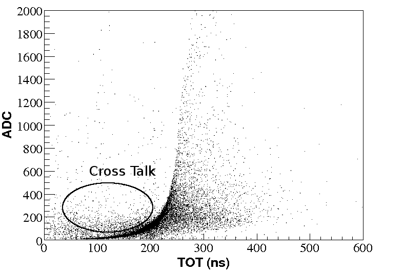
• Hits induced by electrical crosstalk are removed.

The second and third cuts eliminate the majority of dark noise hits. Electrical crosstalk mostly affects

OMs on strings 5 – 10 with communication to the surface on twisted pair cables. The crosstalk cut is

performed in two steps. First, crosstalk hits usually have a large amplitude without a correspondingly

large time over threshold. For each affected OM, this ADC-TOT response is characterized as shown in

figure 4.4, and a crosstalk cut is made. Additionally, crosstalk effects are measured by identifying large

amplitude hits and recording the resulting crosstalk hits in nearby channels, which occur in discrete

Figure 4.4: Identification of crosstalk in ADC vs. TOT distributions for OM 246

during run 9453 in 2005.

time windows relative to the large amplitude hit. A map of time windows for each problematic talker-

receiver channel combination is generated and used to reduce crosstalk. The data is retriggered after

hit selection, and events not passing the multiplicity trigger or string trigger criteria are removed.

4.3 Track Reconstruction

The remaining hits are mostly produced by Cherenkov radiation from energetic particles within

the detector. The Cherenkov photons propagate outward from the particle track, forming a cone with

angle ∼ 41

◦

as illustrated in figure 4.5. For a module a distance d from the muon track, the expected

arrival time of Cherenkov photons emitted at time t

◦

exp

= t

◦

d · cotθ

(4.3)

At distances greater then ∼ 1 – 2 effective scattering lengths from the muon track, the photon flux is

smaller than expected from absorption alone because scattering confines photons to the region near

the track. Photons reaching such distances are delayed by the scattering, and a useful quantity is

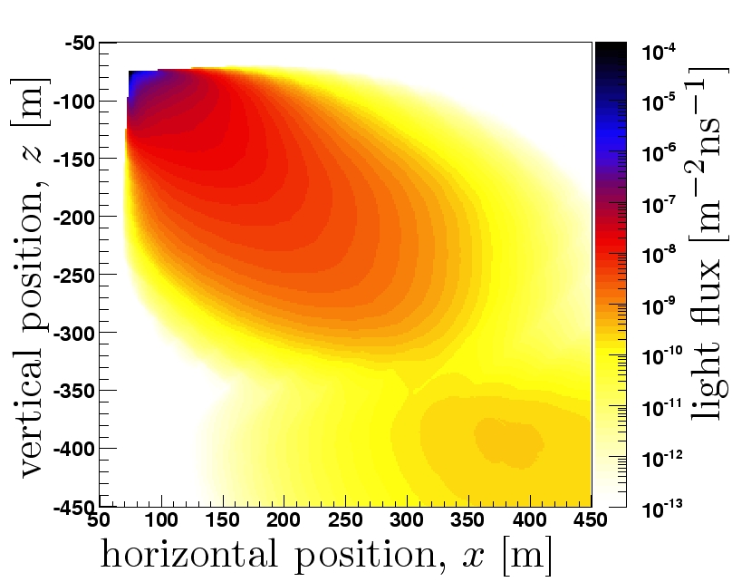
Figure 4.5: Depiction of the Cherenkov cone produced by a relativistic muon (left),

and an instantaneous snapshot of the simulated Cherenkov light flux produced by a

relativistic muon in ice traveling to the upper left at θ = 135

◦

(right), from [101]. The

Cherenkov cone is visible in the top left of the image.

relative arrival time or time residual,

res

= t ? t

exp

(4.4)

Typical time residuals are larger in regions of ice with shorter scattering lengths due to higher

concentrations of imperfections.

4.3.1 Unbiased Likelihood Reconstruction

Given a muon track hypothesis, distances of hits from the track and thus expected Cherenkov

photon arrival times are known; therefore, the time residual for each hit can be computed as described

above. If the likelihood of observing a given time residual is known as a function of distance d from

a hypothesis track for each of the N hits comprising the event, a likelihood can be formulated given

the track zenith (θ), azimuth (φ), and vertex ( r ):

L (θ,φ, r ) =

i =1

P (t

res,i

| d

(θ, φ, r )).

(4.5)

time delay / ns

d = 8m

Delay prob / ns

time delay / ns

d = 71m

Delay prob / ns

−4

−3

−2

−1

200

400

−7

−6

−5

−4

−3

500

1000

1500

Figure 4.6: Time residual distribution from a photon Monte Carlo (black) and Pandel

function (red) for 8 m and 71 m from the muon track, from [93].

Track hypotheses can be ranked by this likelihood, and this formulation can then be used to determine

the best reconstructed track. The time residual distributions P (t

res

| d) can be determined by a photon

Monte Carlo including scattering and absorption. Alternatively, a more convenient approach is the

Pandel function [106], an analytic solution of the photon time residual probability as a function of

distance from the muon track for media with significant absorption and scattering:

P (t

res

| d) =

? ( d/λ )

· t

( d/λ ? 1)

res

N(d) · ?( d/λ)

· e

res

λa

(4.6)

N(d) = e

? d/λ

τ · c

· λ

? d/λ

(4.7)

Comparison with simulation yields a best fit to the free parameters: τ = 557 ns, λ = 33.3 m, and

= 98 m for typical AMANDA ice, shown in figure 4.6. PMT signals in AMANDA have an end-

to-end leading edge timing uncertainty of ∼ 15 ns, and this timing uncertainty is convoluted with

the Pandel function t

res

distributions used in reconstruction [93]. The quantity ? log L is minimized

numerically with respect to the track free parameters θ, φ, and r , yielding a best fit track hypothesis.

Dispersion limits the ability to separate consecutive hits in AMANDA to ∼ 100 ns and ∼ 10 ns for

electrical and optical channels, respectively [93], so many photons are often are combined with the first

hit. Any hits in a given OM subsequent to the first provide much less information for reconstruction

and are disregarded. If many photons are observed in a given module, the first arrives sooner than

Figure 4.7: Pandel likelihood map of ? log L for upgoing event 7442798 in run 9490 of

2005. The minimum is at zenith 145.1

◦

, azimuth 17.45

◦

expected since, on average, the first photon is less scattered. Using only the timing information of

this first photon introduces a mild pathology in the reconstruction of high energy events, which may

yield many photons in any given OM. This effect can be corrected by calculating the time residual

distribution for only the first photon, given N total photons observed in the optical module [93]:

res

| d) = N · P(t

res

| d) ·

∞

res

P (t | d)dt

( N ? 1)

(4.8)

This multi-photoelectron probability is currently computationally intensive and not used for this

analysis, although efforts are underway to improve speed for use in IceCube analysis. Figure 4.7

displays ? log L for an event with respect to zenith and azimuth, fitting only the track vertex r at

each grid point. The event is clearly upgoing, with minimum ? log L at zenith 145.1

◦

, azimuth 17.4

◦

The fit fails to find the true minimum at a portion of grid points for this event, especially at small

zenith angles, due to the complexity of the likelihood space. The detector display of this event along

with the best fit muon track are shown in figure 4.8. To increase the probability of locating the true

minimum, the minimization is repeated 32 times with different starting values for θ, φ, and r . Two of

the seeds come from the best track using the Direct Walk and JAMS algorithms, described in section

4.3.4.

4.3.2 Paraboloid Reconstruction

For point source searches, knowing the angular resolution of obtained events is critical. The

ability to reconstruct muon tracks in AMANDA partially depends on event topology. A muon track

passing through a larger portion of the detector or hitting a larger number of modules should, on

average, reconstruct with better angular resolution due to a longer lever-arm or larger number of

constraining parameters, respectively. Angular resolution can be determined on an event-by-event

basis by examining the likelihood space in the vicinity of the best fit track [107]. As the zenith

and azimuth coordinates (θ, φ) are forced away from the best fit values (θˆ, φˆ), the quantity ? log L

increases parabolically from its minimum as shown in figure 4.7. The likelihood ratio ? 2 · log

L ( θ,φ )

L ( θ

,φ

ˆ)

is evaluated on a grid of zenith and azimuth near the best fit, and the resulting values are fit to a

paraboloid with the form

? 2 · log

L (θ, φ)

L (θˆ, φˆ)

(4.9)

where the x and y axes are fit and do not necessarily correspond to zenith and azimuth. Likelihood

ratio contours enclosing the minimum are chi-square distributed and contain the true direction with

confidence ? 2 · log

L ( θ,φ )

L ( θ

,φ

ˆ)

∼ χ

. Specifically, the ? 2 · log

L ( θ,φ )

L ( θ

,φ

ˆ)

= 1 contour would enclose the

true direction in 39.3% of trials. The paraboloid fit is a convenient approximation of the likelihood

space, summing the complex map of ? 2 · log

L ( θ,φ )

L ( θ

,φ

ˆ)

into three values: σ

, σ

, and an axis rotation

angle. The corresponding track direction probability density estimate can be obtained from the fit

by:

L (θ, φ)

L (θˆ, φˆ)

2 σ

2πσ

(4.10)

4.3.3 Forced Downgoing (Bayesian) Reconstruction

Poor quality downgoing muon events often are misreconstructed as upgoing. Since the number

of downgoing events outnumber the upgoing neutrino events by a factor of ∼ 10

, a fraction of misre-

constructed downgoing events easily overwhelms the much smaller neutrino sample. One method to

remove such events is to reconstruct each as downgoing, and then compare the downgoing likelihood

with the likelihood of the best fit track hypothesis. The downgoing fit is performed in the same

Figure 4.8: Detector display for event 7442798 in run 9490 of 2005. Hit timing

is indicated by the color pattern, with red and blue indicating first and last hits,

respectively. The event is clearly an upgoing muon with a track similar to the shown

best fit.

cos

-1

-0.8 -0.6 -0.4 -0.2

0.2

0.4

0.6

0.8

Prior Weight

-1

Figure 4.9: Zenith prior applied to the likelihood function during Bayesian reconstruc-

tion.

manner as the single-photoelectron likelihood reconstruction, except track zenith is weighted in the

likelihood function by a prior function describing the zenith distribution of downgoing muons, shown

in figure 4.9. The reconstruction is repeated 64 times with different starting values for θ and φ. The

best downgoing track likelihood is compared with the best fit likelihood:

Bayesian

= ? log

L (θˆ

down

, φˆ

down

)

L (θˆ, φˆ)

(4.11)

Good upgoing tracks have large values of Q

Bayesian

since these tracks are not very compatible with a

downgoing hypothesis. Misreconstructed downgoing tracks generally have smaller values of Q

Bayesian

4.3.4 First Guess Algorithms

While the likelihood methods above yield the best angular resolution, it is computationally

not practical to apply a likelihood reconstruction to all of the O(10

) events recorded by AMANDA

each year. Also, the likelihood reconstruction is sensitive to the initial track hypothesis. For these

reasons, we first apply quick, less accurate reconstruction methods, and later we use the results as a

filter for interesting tracks and as seeds for likelihood reconstruction.

4.3.4.1 Direct Walk

Direct Walk is a pattern matching algorithm which identifies tracks using pairs of hits con-

nected by nearly the speed of light (track elements) [93]. Track elements are selected if the following

is satisfied:

| ∆t | <

+30 ns;

d > 50 m,

(4.12)

where d is the distance between the hit OMs. For each track element, we next identify and count the

number of other hits associated with the track element according to the following:

? 30 ns < t

res

< 300 ns;

r < 25 m · (t

res

+ 30)

1 / 4

(4.13)

where r is the distance of closest approach between the track and hit module. High quality track

elements are selected by requiring at least 10 associated hits and an RMS distance along the track

between the track vertex and closest approach to each associated hit greater than 20 m. If multiple

high quality track elements are identified, a cluster search is performed to find the track with the

most other tracks within 15

◦

, and the final track is the average of the tracks within the cluster.

4.3.4.2 JAMS

JAMS is a pattern matching algorithm similar to Direct Walk [108]. For a large number of

track zenith and azimuth hypotheses, we examine each hit for clustering neighbors according to

(∆r)

+(∆z ? c∆t)

< r

max

(4.14)

∆z and ∆r are the distances between the hits along and perpendicular to the track direction, re-

spectively, ∆t is the hit time difference, and r

max

is an arbitrary threshold. A minimum cluster size

of 7 hits is required to keep the track. Each passing track is refined with a simplified log likelihood

reconstruction and then ranked using a neural network. The input parameters include the number

of negative and very large time residuals, and the number of hits >50 m from the track. The final

track is the track with the highest neural net quality.

Chapter 5

Event Selection

As illustrated in figure 5.1, AMANDA records O(10

) events per year, mostly from muons

produced by cosmic ray air showers. Of these, O(10

) are upgoing muons produced by atmospheric

neutrinos, and AMANDA records at most O(10) high quality events per year from extraterrestrial

sources with E

? 2

energy spectra given current limits [26]. We attempt to isolate these neutrino events

from the downward muon background in a computationally efficient manner.

5.1 Data Sets

After accounting for deadtime in data acquisition electronics, nominally ∼ 15% of uptime, we

have accumulated 1387 days (3.8 years) of livetime with 1.29 × 10

events during seven years of

operation (table 5.1). A detector simulation is necessary to optimize the selection of high energy

neutrino-induced muon events. We simulate neutrino events using the software chain described in

Year

Livetime Total Events

Filtered Events

Final Selection

2000

197 d

1.37 B

1.63 M

596

2001

193 d

2.00 B

1.90 M

854

2002

204 d

1.91 B

2.10 M

1009

2003

213 d

1.86 B

2.22 M

1069

2004

194 d

1.72 B

2.09 M

998

2005

199 d

2.06 B

5.21 M

1019

2006

187 d

2.00 B

4.89 M

1050

Total 1387 d

12.92 B

20.04 M

6595

Table 5.1: AMANDA livetime and event totals.

cos

-1

-0.5

0.5

Events

Downgoing Muons

Misreconstructed Muons

Atmospheric Neutrinos

Filtered Data

Final Sample

Diffuse Flux

-2

Figure 5.1: Zenith angle (θ) distributions for data and simulation at several reduction

levels. Reconstructed (solid) and true (fine dotted) zenith angle distributions are shown

for CORSIKA [103] cosmic ray muon simulation at retrigger level, and reconstructed

zenith angle distributions are shown for atmospheric neutrino simulation (dotted) and

data (circles) at retrigger level, filter level, and final selection. We also show the

reconstructed zenith angle distribution of a diffuse E

? 2

neutrino flux at the current

limit [26] using our final selection (dash-dotted).

chapter 3. Each year is simulated with a specific detector configuration to account for changes and

upgrades which occur during the austral summer. We have generated 9 × 10

events per year for ν

fluxes following an E

? 1

energy spectrum, with a zenith angle distribution uniform in cos θ from

◦

< θ < 180

◦

. An event selection sensitive to track-like events is also sensitive to muons produced

by tau decay and even tau tracks at PeV – EeV energies; thus, we have generated similar ν

fluxes. We

have also generated 2 × 10

muon neutrino events per year equally divided into 20 narrow declination

bands, each separated by five degrees, to simulate point sources. The weighting of simulated events

to real fluxes is described in appendix A. Finally, we have generated ∼ 1 × 10

cosmic ray air showers

with CORSIKA [103], used to understand the rejection of background cosmic ray muons.

The event selection is carried out in two phases: First, we apply reconstructions and filter

well-reconstructed downgoing cosmic ray muon events using the Sieglinde [105] software suite. We

then perform the more challenging task of removing cosmic ray muon events wrongly reconstructed

as upgoing. Simulated events are filtered identically to the data.

5.2 Filtering Downgoing Events

For neutrino analysis, the first task is removing the well-reconstructed downgoing muons which

dominate our data, which is a computationally intensive process. The AMANDA raw muon-DAQ

data comprises roughly 2 TB per year. Each year of data contains ∼ 60,000 files, each with ∼ 25,000

events. Each file is processed by Sieglinde [105] according to the following procedure.

5.2.1 Retriggering

After hit cleaning (chapter 4), an event may no longer satisfy the 24-module multiplicity or

string trigger thresholds. Such events are removed to preserve agreement with Monte Carlo. This

retrigger removes roughly 50% of events.

5.2.2 First Guess Reconstruction

Events satisfying the retrigger condition are then reconstructed with the JAMS and DirectWalk

(DW) algorithms, described in chapter 4. The data has been filtered in two separate blocks, 2000-

2004 and 2005-2006, with slightly different event selection strategies. For 2000-2004, our upgoing

Cumulative Event Fraction

0.2

0.4

0.6

0.8

< 30

< 60

< 90

Cumulative Event Fraction

0.2

0.4

0.6

0.8

-2

-2.5

Barr et al. Atm.

Figure 5.2: Angular deviation between neutrino and UL fit track for simulated E

? 2

muon neutrino events from several declination ranges (left) and energy distributions

(right).

event selection requires zenith angles θ

> 70

◦

and θ

JAMS

> 80

◦

. The cuts are interchanged for

2005 and 2006, requiring θ

JAMS

> 70

◦

and θ

> 80

◦

5.2.3 Unbiased Likelihood Reconstruction

The computationally intensive 32-iteration unbiased likelihood (UL) reconstruction is then

applied to surviving events ( ∼ 1% of triggered events). The median accuracy of the UL fit is 1.5

◦

–

2.5

◦

, shown in figure 5.2. With the additional cut θ

> 80

◦

, our upgoing event filter reduces the

downward muon background by nearly a factor of 1000 relative to trigger level (table 5.1). Events

passing the filter are reconstructed with the 64-iteration Bayesian likelihood (BL) and paraboloid

reconstructions.

5.3 Final Event Selection

Several million misreconstructed downgoing muons pass through the filter, still outnumbering

upgoing atmospheric neutrinos by a factor of 1000 (figure 5.1). We remove these misreconstructed

events by applying topological criteria designed to select quality muon tracks. The criteria we use

are the following:

• The Q

Bayesian

likelihood ratio of the UL and BL fits, described in chapter 4. High values of

log(UL/BL) select upgoing events.

• The angular uncertainty of the UL fit, from the paraboloid reconstruction. Misreconstructed

events generally have large angular uncertainty.

• The smoothness, or homogeneity of the hit distribution along the UL track [93]. High quality

events contain photon hits along the entire length of the track and have smoothness values near

zero, whereas hits from misreconstructed events tend to distribute near the beginning or end

of the track and have smoothness values near +1 and ? 1, respectively.

• The UL track direct length, obtained by projecting direct hits backward to the UL track at

the Cherenkov angle and taking the distance along the track between the first and last. We

select direct hits, compatible with relatively unscattered photons and arriving on-time with the

Cherenkov cone, using the time window ? 15 ns < t ? t

< 25 ns [93]. Hits from misre-

constructed events rarely follow the muon-Cherenkov timing pattern over significant distances,

resulting in short lengths.

We select zenith angle dependent cuts using these parameters, assuming our signal is a neutrino

point source with an E

? 2

energy spectrum. The cuts are optimized to minimize the model rejection

factor [109], resulting in the best possible sensitivity to neutrino fluxes. For the zenith angle region

91.5

◦

< θ < 180

◦

, the cuts are (figure 5.3):

log(UL/BL) (Q

Bayesian

) > 34 ? 25 · Φ(cosθ + 0.15)

Angular uncertainty

√

· σ

< 3.2 ? 4 · Φ( ? cosθ ? 0.75)

| Smoothness | < 0.36.

Here Φ(x) = x for positive x, and Φ(x) = 0 for x < 0. We use a support vector machine (SVM)

[110] trained on the above parameters to improve event selection in the near-horizontal region 80

◦

θ < 91.5

◦

. The SVM output is a quality parameter, which is ∼ 1 for signal-like events and ∼ -1 for

background-like events. We apply the following cut on this quality parameter:

SVM Parameter > 1.0 ? 12.08 · Φ(cosθ ? 0.023).

Application of these quality cuts yields 6595 neutrino candidate events [111] (figure 5.6).

Simulated atmospheric neutrino fluxes [69, 70] agree with data in track quality parameter

distributions and zenith angle (figure 5.5) up to a normalization factor within uncertainties on at-

cos

-0.8

-0.6

-0.4

-0.2

Likelihood Ratio (log[UL/BL])

cos

-0.8

-0.6

-0.4

-0.2

Angular Uncertainty (Degrees)

2.6

2.8

3.2

3.4

3.6

3.8

cos

-0.8

-0.6

-0.4

-0.2

Smoothness

0.3

0.32

0.34

0.36

0.38

0.4

0.42

0.44

0.46

0.48

0.5

cos

-0.8

-0.6

-0.4

-0.2

SVM Parameter

-1

-0.5

0.5

1.5

Figure 5.3: Zenith (θ) dependent final cuts for 91.5

◦

< θ < 180

◦

(top and left), and

◦

< θ < 91.5

◦

(bottom right).

data

2000

3000

4000

5000

6000

Ratio Data/MC

0.88

0.9

0.92

0.94

0.96

0.98

Figure 5.4: Ratio of data to simulated atmospheric neutrinos [69] as a function of cut

tightness. As cuts tighten, reducing the number of data and simulated atmospheric

neutrino events, the ratio stabilizes ∼ 3% lower than the value with optimal cuts and

∼ 6100 data events.

mospheric neutrino flux. Application of the filter selection and final quality cuts to this simulation

yields an atmospheric neutrino efficiency of 30% relative to retrigger level for θ > 90

◦

. The contri-

bution of misreconstructed downward muons, estimated by tightening quality cuts until a very pure

atmospheric neutrino sample is obtained, is less than ∼ 3% for θ > 95

◦

(declination δ > 5

◦

), shown

in figure 5.4. Misreconstructed muons are more significant near the equator and dominate events in

the Southern Sky. Evaluation of simulated events retained by the final cuts provides the neutrino

effective area, described in appendix A, shown in figure 5.7 for neutrino energies from 10 GeV to 100

PeV. The simulation is later used to provide flux limits for neutrino point sources.

Likelihood Ratio (log [UL/BL])

Events

Filtered Data

Filtered Atm. Neutrino

Final Data

Final Atm. Neutrino

(Degrees)

Angular Uncertainty

Events

Smoothness

-1

-0.8 -0.6 -0.4 -0.2

0.2

0.4

0.6

0.8

Events

Track Length (m)

100

150

200

250

300

350

Events

SVM Parameter

-5

-4

-3

-2

-1

Events

cos

-1

-0.8

-0.6

-0.4

-0.2

0.2

Events

100

150

200

250

300

350

Data

Barr et al. Atm. Neutrino

Honda (2006) Atm. Neutrino

Figure 5.5: Distributions of data and atmospheric neutrinos at filter level and final

selection level for several parameters and zenith angles θ > 95

◦

(top and left), and

zenith angle distribution for the selected 6595 neutrino candidate events compared

with model predictions [69, 70] for atmospheric neutrinos (bottom right).

Figure 5.6: Equatorial sky map of final 6595 events recorded by AMANDA-II from

2000–2006.

(E/GeV)

Log

-6

-5

-4

-3

-2

-1

< 10

< 35

< 60

< 85

Figure 5.7: Effective area for averaged ν

and ν¯

(solid) and averaged ν

and ν¯

(dashed) neutrino fluxes for several declination ranges.

Chapter 6

Search Method

No TeV neutrino sources have yet been observed. We therefore use discovery-oriented statis-

tical methods to separate any small neutrino point source signal in our data from the atmospheric

neutrino background. To maximize the potential for discovery, we must use all relevant information

from the data in our analysis. Several features distinguish point source signals from the background:

• The event angular distribution. Signal events would cluster around the direction of the neutrino

source with a deviation from the true direction dependent on the detector angular resolution.

• The event energy distribution. The differential energy spectrum of the signal expected from

Fermi acceleration mechanisms is close to E

? 2

, harder than that of atmospheric neutrinos, as

shown in figure 6.1. The differential spectrum of atmospheric neutrinos approximately follows

a power law of E

? 3 . 7

above ∼ 1 TeV.

• The event time distribution. Signal events would be distributed nonuniformly in time from

sources which are periodic, flaring, or one-time bursts. The atmospheric neutrino event rate is

generally constant over time.

The most straightforward way to incorporate this information into a search method is through

a binned search, using an angular bin with radius comparable to the detector angular resolution

to select events. A neutrino source would produce an event excess above the atmospheric neutrino

background event expectation for the bin, with a significance given by binomial statistics. Additional

cuts may be used to select energetic events or, in the case of time dependence, events within a time

/GeV)

Log

(E)]

dN/d[log

Atmospheric Neutrino Flux

Neutrino Flux

-2

Figure 6.1: Energy distribution of events passing selection criteria for simulated at-

mospheric neutrino background [69] in a 3.5

◦

bin and an E

? 2

point source with flux

+ ν

= 10

? 10

TeV cm

? 2

? 1

. Such a source would be detected at 5σ in approxi-

mately 40% of trials.

window to reduce the background and increase the probability that a given neutrino flux will be

significant. Two general problems reduce the performance of binned methods:

1. The information reduction problem : All of the event information is reduced to a binary

classification; either the event passes the cuts and is counted, or it does not. Information is

lost that alternatively could indicate the relative agreement of each event with a neutrino point

source signal or background. For example, events at the edge of a search bin are not as indicative

of a point source as events near the center, but are counted the same. More importantly, muon

events with energies above the cut threshold are counted the same; however, since the spectra

of an E

? 2

signal and the atmospheric neutrino background differ by ∼ E

1 . 7

, muons with energy

well above the cut threshold are orders of magnitude more compatible with a point source signal

than with background.

2. The optimization problem : The cuts, including the angular bin radius, must be optimized

given a specific point source signal hypothesis. If the hypothesis does not accurately describe

the signal, the cuts may not be optimal. Additionally, the cuts which optimize sensitivity [109]

(i.e. set the best limits) do not maximize the probability of discovering a signal, and therefore

a choice must be made to sacrifice either sensitivity or discovery potential.

We avoid these problems entirely by using a maximum-likelihood search method [112], incorporating

event angular and energy information on an event-by-event basis. Similar methods have been pro-

posed [113, 114, 115]. In appendix B we expand this method to include time information for sources

with time-dependent fluxes.

6.1 Maximum Likelihood Search Method

At any direction in the portion of the sky observed by AMANDA, the data can be modeled

by two hypotheses:

• H

: The data consists solely of background atmospheric neutrino events, i.e. the null hypothesis.

• H

: The data consists of atmospheric neutrino events as well as astrophysical neutrino events

produced by a source with some strength and energy spectrum.

If H

and H

are described by probability density functions (PDFs) over parameters from the data,

the likelihood of obtaining the data is calculable given either hypothesis. We use a likelihood ratio

test with the standard log-likelihood test statistic

λ = ? 2log

P (Data | H

)

P (Data | H

)

(6.1)

Larger values of λ indicate the data is less compatible with the background hypothesis H

. The PDFs

P (Data | H

) and P (Data | H

) are calculated using knowledge of the spatial and energy distribution

of events from background and simulated neutrino point sources.

6.1.1 Confidence Level and Power of a Test

The utility of a statistical test is measured by the rate of type-I and type-II errors (α and β),

known respectively as the confidence level (CL) and power (1 - β) of the test:

• Type-I Error : H

is rejected when H

is true, i.e. a false discovery claim.

• Type-II Error : H

is not rejected when H

is false.

A tradeoff exists between CL and power, and reducing the probability of false discovery necessarily

reduces the power to discover any signal present in the data. The accepted CL threshold necessary

to claim a discovery is generally 5σ, a false discovery rate of 5.73 × 10

? 7

, and a weaker 3σ result

(2.7 × 10

? 3

) may be considered evidence of a signal. At a given CL, power is dependent on the

strength of the signal; weaker signals are less likely to be detected. The flux necessary to reach a

given level of power (e.g. 50%, 90%) at a given CL is the discovery potential, a figure of merit for

the search. Finally, 1σ (68%) and 90% CL are often used as uncertainty bounds on the physical

parameters of H

6.1.2 Search Method

We consider a search method for neutrino emission from a fixed point in the sky ?x

using the

set of 6595 AMANDA muon events. Each muon event has an energy estimate and a reconstructed

position ?x

, separated from the source position by an angular distance Ψ

= | ?x

? ?x

| . The signal

PDF describes the likelihood of observing the event energy estimate and angular separation Ψ

given

a point source at position ?x

, and is a product of spatial and energy likelihood terms:

= L (Ψ

) × L (E

(6.2)

6.1.2.1 Spatial Likelihood

Each event has an angular uncertainty about the best fit position ?x

related to the event

topology (section 4.3.2), and we incorporate this angular uncertainty into the analysis. We use the

paraboloid reconstruction angular uncertainties, σ

and σ

, in a circularized fashion:

√

· σ

(6.3)

The angular error estimate σ

is an accurate approximation of the much more complex reconstruction

likelihood space, shown for example in figure 4.7. The spatial PDF is the relative likelihood of the

true track direction being ?x

, given both the angular distance Ψ

from the event best fit and event

angular uncertainty σ

, which is a normalized two-dimensional Gaussian:

L (Ψ

) =

2πσ

Ψ2

2 σ

(6.4)

Angular Deviation (Degrees)

0.5

1.5

2.5

3.5

4.5

Probability Density

0.2

0.4

0.6

0.8

1.2

0.6

≤

0.4

0.9

≤

0.8

1.4

≤

1.3

2.0

≤

1.9

/GeV)

log

Probability Density

0.1

0.2

0.3

0.4

0.5

0.6

0.7

0.8

≤

Nch

≤

Nch

≤

105

≤

Nch

≤

200

≤

Nch

≤

185

Figure 6.2: Distributions of angular deviation between true and reconstructed tracks

for simulated neutrino-induced muon events over several ranges of estimated angular

uncertainty (left), and muon energy distributions for four ranges of Nch (right).

Distributions of the angular deviation between true and reconstructed tracks of simulated muons in

figure 6.2 show the correlation between estimated angular uncertainty and track reconstruction error.

6.1.2.2 Energy Likelihood

The amount of light deposited in the detector depends strongly on muon energy above ∼ 1 TeV,

and the number of hit modules (Nch) provides an approximate measure of event energy. Distributions

of muon energy for several ranges of Nch are shown in figure 6.2. As an energy estimator, Nch yields

a 1σ uncertainty in log

) of 0.65. Astrophysical neutrino spectra are assumed to follow a power

law E

? γ

with γ ∼ 2, so the meaningful quantity is the likelihood of obtaining the event Nch value

(Nch

) given a spectral index. This energy PDF is

L (E

) = P(Nch

| γ) =

P (Nch

| E

)P (E

| E

)P (E

| γ)dE

(6.5)

The convolution is done by the neutrino simulation. Nch distributions of any spectral index are

produced by weighting the simulation according to the spectral index (appendix A). From these sim-

ulations, we tabulate Nch probabilities for spectral indices 1 ≤ γ ≤ 4 and for atmospheric neutrinos

[69] in bins of 0.01, shown in figure 6.3. For example, a muon event with an Nch value of 200 is a

Nch

100 120 140 160 180 200

Probability Density

-6

-5

-4

-3

-2

Atmospheric

Signal

-2

Signal

-2.5

Signal

-3

Figure 6.3: Simulated Nch distributions for atmospheric neutrinos [69] and E

? 2

, E

? 2 . 5

and E

? 3

power law neutrino spectra.

factor of ∼ 100 more likely to be from an E

? 2

source than from the atmospheric background.

6.1.2.3 Signal and Background PDFs and the Test Statistic

The final signal PDF is the product of the spatial and energy PDFs,

(Ψ

, σ

, Nch

, γ) =

2πσ

Ψ2

2 σ

× P(Nch

| γ).

(6.6)

The atmospheric neutrino background is uniform in right ascension and roughly uniform over a narrow

declination band. Similar to the signal PDF, the normalized atmospheric neutrino background PDF

is the product of the spatial and energy terms:

(Nch

) =

Ω

band

× P (Nch

| Atm

(6.7)

We only consider events within a declination band of ± 8

◦

of the search position ?x

, much larger

than the declination-dependent AMANDA resolution of 1.5

◦

- 2.5

◦

. The normalization constant

Ω

band

is the solid angle of this band. If enough events are recorded, the probability P(Nch

| Atm

)

can determined from an Nch histogram directly obtained from off-source data. This is preferable,

especially in the case the data contains misreconstructed downgoing muons, which tend to have higher

Nch values than atmospheric neutrinos; however, our sample of 6595 events is not sufficient at large

Nch values, and we use probabilities tabulated from simulation.

Spectral Index

1.5

2.5

3.5

Likelihood Penalty

-3

-2

-1

Figure 6.4: Likelihood penalty limiting γ to the range 2.0 < γ < 2.7.

We model the data as a two-component mixture of signal and background events, i.e. the data

is a combination of S

and B

. The full-data likelihood is the product of this mixture likelihood over

N total events in the declination band:

L (?x

, n

, γ) =

i =1

+ (1 ?

) B

(6.8)

where

is the unknown fraction of signal events. The likelihood is maximized with respect to n

and γ, giving the best fit signal hypothesis and best estimates of the number of signal events nˆ

and

spectral index γˆ. We first perform a grid search in γ to determine a starting value, and then the

maximization is done by numerically minimizing the quantity ? 2 log L with the MIGRAD minimizer

from the MINUIT library [116]. We limit γ to the approximate range 2.0 < γ < 2.7 with a top-

hat Gaussian likelihood penalty, shown in figure 6.4. The penalty improves discovery potential for

the expected source spectra, shown in figure 6.6, by discriminating against the γ ∼ 3.7 atmospheric

neutrino background. Finally, a lower limit exists for the fraction of signal events

, below which

? 2 log L becomes infinite, so we place an explicit bound on the minimization:

> max

> B

(6.9)

If no events satisfy S

> B

, ? 2log L monotonically increases with

, and the minimization uses

> ? 1 as a lower bound. This pathological case occurs when no events are present within an angular

distance comparable to the angular resolution and can effectively be ignored. Alternative likelihood

maximization techniques, including expectation-maximization (EM) [115], have been proposed and

should yield equivalent results. The test statistic is the comparison of the background-only likelihood

(i.e. n

= 0) with the best fit signal likelihood, using nˆ

, and γˆ:

λ = ? 2 · sign(nˆ

) · log

L (?x

, 0)

L (?x

, nˆ

, γˆ )

(6.10)

We include the factor sign(nˆ

) to differentiate negative and positive excesses.

Finally, it is preferable to include event energy information when the distribution of energies

from signal events differs considerably from background. When the energies are comparable, e.g.

in a search for neutrinos from WIMP annihilation (chapter 8), the inclusion of energy information

provides no benefit. The signal and background PDFs without energy information are

(Ψ

, σ

) =

2πσ

Ψ2

2 σ

(6.11)

Ω

band

(6.12)

resulting in simpler expressions for L .

6.2 Evaluating Significance and Discovery Potential

Given an observation of the test statistic λ, we compute significance by comparing the observed

value with the distribution of test statistic values obtained from data randomized in right ascension,

which is analogous to the background-only hypothesis. We obtain this distribution by performing

5 × 10

iterations of the likelihood search using randomized data, then recording the value of λ at an

arbitrary point for each of 20 declination bands spanning -7.5

◦

< δ < 87.5

◦

. Larger values of λ are

less compatible with the background hypothesis, so CL thresholds of λ are obtained by integrating

the distribution backward. The 3σ threshold of λ is taken directly from the integral distribution, and

because of statistical uncertainty, an exponential fit is done on the tail of the integral distribution

to obtain the 5σ threshold, shown in figure 6.5. The integral distribution approximately follows a

chi-square ( ∼

We then obtain distributions of the test statistic given a signal of known strength. For each

declination band, we perform 50,000 iterations of the likelihood search for 80 values of signal strength

from 1 to 80 added signal events. For each iteration, signal events are chosen by a weighted random

)

-7

-6

-5

-4

-3

-2

-1

dP/d

0.01

0.02

0.03

0.04

0.05

0.06

0.07

0.08

0.09

5σ

BG + 6 Signal Events

BG + 12 Signal Events

BG + 18 Signal Events

Figure 6.5: Integral distribution of the test statistic for background at δ=42.5

◦

with

3σ and 5σ thresholds indicated and statistical uncertainty shaded in gray (left), and

distribution of the test statistic for background and 6, 12, and 18 added signal events

at δ=42.5

◦

(right).

selection from neutrino simulation with a power-law energy spectrum, usually E

? 2

. For each value

of signal strength, a fraction of trials F

pass the 3σ or 5σ CL thresholds, shown in figure 6.5. From

this, we compute the detection probability F(µ), the fraction of trials passing 3σ or 5σ CL thresholds

given a Poisson mean number of events µ:

F(µ) =

i =0

× P(i | µ)

(6.13)

where P(i | µ) is the Poisson probability of observing i events given mean µ. The mean number of

events is directly proportional to the neutrino flux, and the fraction F(µ) is the power at 3σ or 5σ CL

thresholds. The power of this analysis is shown in figure 6.6, and 13 – 14 signal events are required

to detect a neutrino point source at 5σ CL in 50% of trials. For E

? 2

spectra, the use of energy

information in the likelihood reduces the mean number of events necessary to discover 50% of sources

at 5σ CL by 35%, shown in figure 6.6. The improvement increases for harder spectra, and is close to

zero for soft spectra ∼ E

? 3

– E

? 3 . 5

The proportionality factors between mean number of signal events and point source neutrino

flux are determined by simulation. The model discovery potential (MDP) is the flux necessary to

achieve a given CL and power, and is shown in figure 6.8 at 3σ and 5σ CL and 90% power as a

Events

-2

Poisson Mean E

Detection Probability

0.2

0.4

0.6

0.8

=7.5

=37.5

=67.5

=7.5

=37.5

=67.5

Spectral Index

1.5

2.5

3.5

Poisson Mean Events

Penalized Search 5

Unpenalized Search 5

Search Without Nch 5

Figure 6.6: Power (detection probability) of the AMANDA 2000-2006 analysis at

3σ and 5σ CL as a function of mean signal strength (left), and comparison of 5σ

CL, 50% power mean event thresholds for the analysis with spectral index constraint,

without constraint, and not using Nch information as a function of spectral index for

the AMANDA 2006 data (right).

function of declination.

6.3 Evaluating Flux Limits

Flux limits are evaluated using the frequentist Feldman-Cousins [117] technique. The observ-

able for this analysis is the test statistic, which is continuous, rather than an integer number of events.

We therefore generate our own confidence bands rather than using the precomputed tables of Feldman

and Cousins. Our confidence limits constrain the mean number of signal events and are converted to

flux limits with proportionality constants determined from simulation. We use D = sign(λ) ·

| λ | as

the observable rather than λ to condense the observable axis. We create a 2-dimensional histogram

with 3000 bins on the observable axis from -10 to 40 in D and 5000 bins on the mean signal strength

axis from 0 to 50 events. We then fill the histogram with distributions of D for each of the 5000

values of the mean signal strength µ. For a given mean signal strength µ, the probability of obtaining

D is

P( D| µ) =

i =0

P( D| i) × P(i | µ)

(6.14)

sign(

-4

-2

Mean Events

Figure 6.7: Feldman-Cousins 90% confidence level band for δ=42.5

◦

where P( D| i) is the probability of obtaining D given i signal events, and P(i | µ) is the Poisson

probability obtaining i signal events given µ. For each observable bin, the maximum value of

P( D| µ) = P( D| µ

best

) is recorded. Acceptance intervals are constructed for each value of µ by

ranking each observable bin by the ratio

L = P ( D| µ)/P ( D| µ

best

(6.15)

The bin with the maximum value of L is included in the acceptance interval, and then the interval

is expanded on either side by choosing the bin with the largest L . The expansion continues until

the integrated probability in the acceptance interval reaches 90% CL. The band coverage is then

increased until all values of D intersect the band exactly twice, i.e. the band is monotonic. Figure

6.7 shows an example of the final confidence band created. Upper and lower limits in signal strength

given an observation of D are the upper and lower intersection, respectively of the vertical line

containing D and the band. Sensitivity is the average upper limit obtained from the D distribution

given background alone (i.e. P ( D| 0)). This procedure is repeated for each of the 20 declination bands

and is shown in figure 6.8. The declination average sensitivity to muon neutrino fluxes following an

? 2

energy spectrum is 2.5 × 10

? 11

TeV cm

? 2

? 1

sin

-0.2

0.2

0.4

0.6

0.8

-1

-2

TeV cm

-11

/dE / 10

90% CL

99% CL

sin

-0.2

0.2

0.4

0.6

0.8

-1

-2

TeV cm

-11

/dE / 10

Figure 6.8: Sensitivity (left) and MDP at 90% power (right) for fluxes from point

sources of muon neutrinos following E

? 2

energy spectra as a function of declination.

6.4 Estimating Spectral Index

Since source spectral index is a free parameter and fitted to the most likely value, the method

provides an estimate of the spectral index of any discovered sources. The estimation becomes more

accurate as the number of signal events increases, with 1σ uncertainty in spectral index improving

from ∼ 0.3 for 15 signal events to ∼ 0.15 for 50 signal events, as shown in figure 6.9 for simulated

? 2

and E

? 2 . 5

source spectra. Source strength and spectral index can be constrained simultaneously

from the likelihood function. Likelihood ratio contours enclosing the best fit minimum (nˆ

and γˆ) are

approximately chi-square distributed, with ? 2 · log

L ( n

,γ )

L ( n ˆ

,γ ˆ)

∼ χ

. Figure 6.9 shows 1σ CL contours

for 10 simulated experiments with 50 added signal events each, with E

? 2

energy spectra. 70% of the

circles contain the true point, consistent with the chosen CL.

Finally, a small offset exists between the mean of γˆ returned from the likelihood minimization

and the true value, as can be seen in figure 6.9. The offset is declination dependent and results from

small differences in the Nch distribution with declination; it can be measured and calibrated away.

Number of Signal Events

Spectral Index

1.4

1.6

1.8

2.2

2.4

2.6

2.8

3.2

Neutrino

-2

Neutrino

-2.5

Spectral Index

1.4

1.6

1.8

2.2

2.4

2.6

Mean Signal Events

True Point

Figure 6.9: Spectral index estimation for simulated experiments with 10 to 80 added

? 2

or E

? 2 . 5

simulated signal events at δ = 22.5

◦

(left). Error bars indicate the 1σ

uncertainty in spectral index. Confidence contours for 10 simulated experiments at

δ = 22.5

◦

(right). The dashed circles represent the 1σ confidence level simultaneous

estimation of signal strength and spectral index for each trial.

Chapter 7

Search for Neutrino Point Sources

We apply the method described in the previous chapter to three separate searches for ∼ TeV

neutrino point sources in the Northern Sky, including an unbiased search, a search based on a list

of interesting astronomical objects, and a search for a cumulative signal from six Milagro hotspots.

Finally, we perform a search for event correlations at small angular scales. We calculate significances

and neutrino flux limits, taking into account the systematic uncertainties in our simulation.

7.1 Systematic Uncertainties

Systematic uncertainties affecting our event expectations from E

? 2

fluxes are itemized in

table 7.1. Most of these uncertainties originate in our detector simulation and can be constrained by

comparing simulated atmospheric neutrinos and downgoing muons with data. Especially, downgoing

muons provide high statistics, and comparison with CORSIKA simulation allows an accurate estimate

of these uncertainties.

7.1.1 Optical Module Sensitivity

The sensitivity of optical modules is not absolutely known and is one of the largest systematic

uncertainties, directly affecting the trigger rate for near-threshold events. Simulations show this

trigger rate effect is zenith dependent, and thus any global change in optical module sensitivity alters

the zenith distribution of downgoing muons [118]. The optical module sensitivity in downgoing muon

simulations is shifted until the simulated zenith distribution matches data, giving a best fit global

optical module sensitivity offset of

? 10

% and impacting the event expectation from E

? 2

neutrino

Source

Magnitude

Optical module sensitivity

? 9

Photon propagation

± 5 %

Event selection bias

? 7

Event reconstruction

? 7

Rock density and neutrino cross section

± 8 %

Other known sources

< 4 %

Total

+ 10

? 17

Table 7.1: Systematic uncertainties in event rate expectations for point sources with

? 2

energy spectra.

fluxes by

? 9

7.1.2 Photon Propagation

The depth dependence in scattering and absorption coefficients of South Pole ice [87] are

ignored in our simulation. A more recent photon propagation code [101] which includes this depth

dependence is now available. A comparison of these simulations yields an event rate uncertainty of

± 5% when applied to E

? 2

neutrino fluxes [118]. The uncertainties in optical module sensitivity and

photon propagation are not fully independent and can alternatively be constrained simultaneously.

This is done in [119] and chapter 8, and yields similar results.

7.1.3 Event Selection and Reconstruction

Simulated distributions of event selection parameters show small offsets relative to distribu-

tions obtained from data. Particularly, distributions of smoothness and angular uncertainty (σ

) are

shifted by ∼ 5-10% for simulated downgoing muons, and by ∼ 7-10% for atmospheric neutrinos in the

final sample [118]. In both cases, the shifts show fewer data events are selected than suggested by

simulation, and thus the event selection efficiency is overestimated. Scaling the simulation by these

factors reduces event expectations from E

? 2

neutrino fluxes by 7% [118], so we assume an uncertainty

? 7

%. The bias in reconstruction uncertainty also suggests our reconstruction of simulated events

is overly accurate and the point spread of E

? 2

neutrino point sources is underestimated. Increasing

our simulated point spread by 8% results in E

? 2

neutrino flux limits 7% higher, so we assign an

uncertainty of

? 7

%. The absolute pointing accuracy of AMANDA has been confirmed by observing

downgoing muon events coincident with well-reconstructed air showers recorded by SPASE [93] and

events coincident with IceCube.

7.1.4 Rock Density, Neutrino Cross Section, and Other Sources of Uncertainty

The rate of neutrino induced muons passing through the detector depends on the composition

of the surrounding medium and the neutrino-nucleon charged current cross section. The density

of underlying bedrock at the South Pole is known to 10% uncertainty [118]. Adjusting the bedrock

density in simulations by 10% affects the E

? 2

neutrino event expectation by at most 7% [118] for near

vertical events, which pass through the most bedrock. The neutrino-nucleon charged current cross

section uncertainty is estimated by error analysis of CTEQ6 parton density functions [120], and the

resulting uncertainty on E

? 2

event rates is less than 3% [118] at TeV – PeV energies. Other known

sources of systematic uncertainty, including uncertainties in optical module timing resolution and

uncertainties associated with the search method, total less than 4%. The total systematic uncertainty

+10

? 17

% is incorporated into our Feldman-Cousins [117] limit calculations using the method of Conrad

et al. [121] as modified by Hill [122].

7.2 Search for Point Sources

7.2.1 Search Based on a List of Candidate Sources

We first apply the search to a predefined list of 26 interesting coordinates (table 7.2), including

locations of AGN, supernova remnants, microquasars, and other energetic phenomena. For each

source location, we compute the value of the unbinned search test statistic λ and compare to data

randomized in right ascension to compute significance. Limits on ν

+ ν

fluxes at 90% confidence

level and chance probabilities (p) are shown in table 7.2. Limits on ν

fluxes alone correspond to

half these values. The highest significance is found for Geminga with p = 0.0086. The probability of

obtaining p ≤ 0.0086 by chance for at least one of 26 sources is 20% and is therefore not significant.

7.2.2 Search of the Northern Sky

We then apply the search to declinations ? 5

◦

< δ < 83

◦

on a 0.25

◦

× 0.25

◦

grid. The region

above declination 83

◦

is left to a dedicated search for WIMP annihilation at the center of the Earth

[123]. For each grid point, we similarly compute a flux limit and significance (figure 7.1). We find a

maximum pre-trial significance of p = 7.4 × 10

? 4

at δ = 54

◦

, α = 11.4h. We account for the trial factor

associated with the all sky search by comparing the maximum pre-trial significance to the distribution

of maximum pre-trial significances obtained from sky maps randomized in right ascension. We find

95% of sky maps randomized in right ascension have a maximum significance of at least p = 7.4 × 10

? 4

(figure 7.1). Sensitivity and flux limits are summarized in figure 7.3.

7.2.3 The Cygnus Region

The region near Cygnus deserves special attention, as several TeV gamma ray sources exist

in this area. Most interesting are the galactic sources discovered by Milagro [18], including MGRO

J2019+37 and MGRO J2031+41, which are detected at 10.4 σ and 6.6 σ pre-trial significance re-

spectively. Subsequent observation of these sources by VERITAS [125] and MAGIC [83] suggest they

have hard energy spectra with γ ∼ -2. Further observation by Milagro has revealed diffuse emission

from the Cygnus region [126]. Such observations suggest these TeV sources may be galactic cosmic

ray accelerators and should be accompanied by neutrino emission. Several predictions of neutrino

fluxes have been made for these sources [51, 127], which are generally about an order of magni-

tude weaker than the sensitivity of this analysis. Pre-trial significances from our analysis of this

region are shown in figure 7.4 along with the significance map from Milagro [81]. The maximum pre-

trial significance observed by AMANDA is ∼ 2.2 σ, which is not significant considering trial factors

over the entire Northern Sky. A 1.5 σ excess of events is observed from the general Cygnus region

(72

◦

< l < 83

◦

, ? 3

◦

< b < 4

◦

). If these small excesses are due to sources, they will be discovered by

IceCube within the next few years.

7.2.4 Milagro Source Stacking

Since the galactic TeV gamma ray sources observed by Milagro are promising TeV neutrino

candidates, we improve our ability to detect a weak signal from these objects by combining obser-

Candidate

δ(

◦

) α(h)

Ψ(

◦

) N

3C 273

2.05 12.49 8.71

0.086

2.1

SS 433

4.98 19.19 3.21

0.64

2.2

GRS 1915+105

10.95 19.25 7.76

0.11

2.3

M87

12.39 12.51 4.49

0.43

2.3

PKS 0528+134

13.53 5.52 3.26

0.64

2.3

3C 454.3

16.15 22.90 2.58

0.73

2.3

Geminga

17.77 6.57 12.77 0.0086

2.3

Crab Nebula

22.01 5.58 9.27

0.10

2.3

GRO J0422+32

32.91 4.36 2.75

0.76

2.2

Cyg X-1

35.20 19.97 4.00

0.57

2.1

MGRO J2019+37 36.83 20.32 9.67

0.077

2.1

4C 38.41

38.14 16.59 2.20

0.85

2.1

Mrk 421

38.21 11.07 2.54

0.82

2.1

Mrk 501

39.76 16.90 7.28

0.22

2.0

Cyg A

40.73 19.99 9.24

0.095

2.0

Cyg X-3

40.96 20.54 6.59

0.29

2.0

Cyg OB2

41.32 20.55 6.39

0.30

2.0

NGC 1275

41.51 3.33 4.50

0.47

2.0

BL Lac

42.28 22.05 5.13

0.38

2.0

H 1426+428

42.68 14.48 5.68

0.36

2.0

3C66A

43.04 2.38 8.06

0.18

2.0

XTE J1118+480

48.04 11.30 5.17

0.50

1.8

1ES 2344+514

51.71 23.78 5.74

0.44

1.7

Cas A

58.82 23.39 3.83

0.67

1.6

LS I +61 303

61.23 2.68 14.74

0.034

1.5

1ES 1959+650

65.15 20.00 6.76

0.44

1.5

Table 7.2: Flux upper limits for 26 neutrino source candidates: Source declination,

right ascension, 90% confidence level upper limits for ν

+ ν

fluxes with E

? 2

spectra

+ ν

≤ Φ

× 10

? 11

TeVcm

? 2

? 1

) over the energy range 1.9 TeV to 2.5 PeV,

pre-trial significance, median angular resolution of primary neutrino, and number of

events inside a cone centered on the source location with radius equal to the median

point spread. Since event energy is an important factor in the analysis, the number of

nearby events does not directly correlate with pre-trial significance.

Figure 7.1: Sky map of significances (σ) obtained in the full-sky search excluding trial

factors (top), and sky map of ν

+ ν

flux upper limits for an E

? 2

energy spectrum

(10

? 11

TeV cm

? 2

? 1

) over the energy range 1.9 TeV to 2.5 PeV (bottom).

Maximum Significance (-log

Trials

100

95%

Figure 7.2: The distribution of maximum significances obtained from 1000 randomized

sky maps, with the obtained significance p = 7.4 · 10

? 4

dotted.

Declination (Degrees)

-80

-60

-40

-20

)

-1

-2

/dE (TeV cm

-12

-11

-10

-9

-8

MACRO 6 Yr.

Super-K 4.5 Yr.

AMANDA 3.8 Yr.

AMANDA 3.8 Yr. Sensitivity

IceCube 9 String (137 d. Sens.)

IceCube 22 String (276 d. Sens.)

IceCube 80 String (1 Yr., Pred.)

ANTARES (1 Yr., Pred.)

Figure 7.3: E

? 2

flux limits for this work, MACRO [28], and Super-K [29], E

? 2

sensitivity for this work and the IceCube 9-string analysis [92], and predicted sensitivity

for ANTARES [124] and IceCube. Our ν

+ ν

limits are divided by 2 for comparison

with limits on only ν

Figure 7.4: Pre-trial significance map of the Cygnus region in TeV gamma rays by

Milagro (from [81], top), and significance map of the same region from AMANDA

(bottom).

vations for several potential sources in a so-called stacking analysis. The improvement is ∼

√

N for

combining N sources of similar strength, with less improvement if one source is much stronger than

average. We include five of eight sources and source candidates observed by Milagro with significance

above 5σ before considering trial factors, including MGRO J2019+37 and MGRO J2031+41, two

areas of lesser significance near Cygnus, and the source MGRO J1908+06. Observations by HESS

[82] indicate MGRO J1908+06 has a hard energy spectrum with γ ∼ -2, similar to the sources near

Cygnus. We add a hot spot near δ = 1

◦

, α = 19h [81], which may be associated with a large neutrino

flux if confirmed as a source [51]. We exclude the three regions with pulsar-wind nebula counterparts,

C3, C4, and the Crab Nebula, which are considered weaker candidates for significant hadron acceler-

ation [51]. We adapt a method developed by HiRes [128] to perform our maximum likelihood search

simultaneously for all six source locations, resulting in the slightly modified likelihood function

L =

i =1

j =1

+(1 ?

) B

(7.1)

where S

is the signal probability density of the i

event evaluated for the j

source. Significance

is again computed by comparing the obtained test statistic value to the distribution obtained from

data randomized in right ascension. We observe a small excess with a chance probability of 20%.

The 90% confidence level upper limit obtained on the mean ν

flux per source is 9.7 × 10

? 12

TeV

? 2

? 1

, considerably more stringent than the non-stacking limits for these sources.

7.2.5 Search for Event Correlations at Small Angular Scales

One additional signal scenario may be several sources producing only a few events each in

AMANDA, too few to be considered significant individually in an all-sky analysis. However, the

cumulative event clustering at small angular scales from all sources may yield an observable signal.

We search for such a signal by counting the number of event pairs in the data given angular and

energy constraints. We consider correlations of events at all angular distances up to 8

◦

and over

a range of energy thresholds, using the number of modules hit as an energy parameter. For each

threshold in angular distance and number of modules hit, we count the number of event pairs in the

data and compare with the distribution of pairs from data randomized in right ascension to compute

significance. The highest obtained significance is p = 0.1 with a threshold of 146 modules hit and 2.8

◦

Figure 7.5: Significance (σ) of the observed number of event pairs with respect to

thresholds on angular separation and number of modules hit.

angular separation, where we observe two event pairs. The probability of observing this maximum

significance by chance, including trial factors from the sliding angular and energy thresholds, is 99%

and is not significant. This hypothesis can additionally be tested by decomposing the data into

spherical harmonics and searching for excesses at large l, indicating structure at small angular scales.

A search using this technique [129] has revealed no excess.

Chapter 8

Search for WIMP Dark Matter from the Sun

An additional unknown component of the universe is the missing, non-luminous mass suggested

by a wide variety of astronomical observations. The most recent measurements from WMAP [130]

and SDSS [131] indicate this dark matter is cold, i.e. non-relativistic, and has a density Ω

∼ 0.2

(Ω

= 0.1050 ± 0.004), significantly larger than that of baryonic matter Ω

∼ 0.04 (figure 8.1).

Since the universe is very nearly flat (Ω

tot

∼ 1), the vast majority of the universe is dark energy, with

Ω

∼ 0.76.

Weakly interacting massive particles (WIMPs) with electroweak scale masses are currently a

favored explanation of cold dark matter. Such particles must be stable or have a lifetime comparable

to the age of the universe, and would interact with luminous matter gravitationally and through weak

interactions. The minimal supersymmetric standard model (MSSM) provides a natural candidate,

the lightest neutralino [132]. An additional candidate is the lightest Kaluza-Klein particle (LKP),

predicted by models of universal extra dimensions [133]. A large range of potential WIMP masses

exists, with lower bounds of 47 GeV [2] and 300 GeV [134] on the lightest neutralino and LKP,

respectively, imposed by accelerator-based analyses. The upper limit of WIMP masses is several

TeV, as higher masses overpredict the observed dark matter density [135].

8.1 Detection of WIMP Dark Matter

If WIMPs comprise dark matter, they are present in our galaxy, orbiting the galactic center

with mean velocity ∼ 270 km s

? 1

and density ∼ 0.3 GeV cm

? 3

[136]. Searches for these WIMPs

generally follow two philosophies. First, WIMP-nucleon elastic scattering events may be directly

Figure 8.1: Combined measurements from WMAP and the SDSS luminous red galaxy

(LRG) survey, showing energy vs. matter density (left), and baryon vs. total matter

density (right), from [131].

observable in Earth-based detectors. Such direct detection experiments observe the recoil of target

nuclei through ionization, scintillation, and phonons. The WIMP-nucleus cross section contains spin-

independent (SI) and spin-dependent (SD) components, and it is not known which component is

dominant. The most sensitive direct detection experiments [137, 138] use germanium and xenon

nuclei, respectively, as targets. The SI cross section scales σ

∼ A

, while the SD cross section does

not scale as such with A; thus, direct detection experiments using targets with large A, including

germanium and xenon, are much more sensitive to SI couplings. Results from direct detection

experiments are summarized in figure 8.2. Multi-ton liquid xenon or liquid argon detectors (e.g.

[139]) should improve current direct detection limits by a factor of 1000 in the next 10 – 15 years.

Alternatively, WIMP annihilation or decay may produce a flux of standard model particles

observable at Earth. WIMP annihilation should produce W

, ZZ, quark, and heavy lepton pairs.

Decay of these particles ultimately produces photons, neutrinos, and electrons and positrons; thus

a WIMP signal would appear as an electron and positron cosmic ray excess or a flux of photons

or neutrinos. Such an excess of cosmic ray electrons and positrons from ∼ 100 GeV – 1 TeV has

WIMP mass [GeV/c

]

Spin−independent cross section [cm

]

−44

−43

−42

−41

Baltz Gondolo 2004

Roszkowski et al. 2007 95% CL

Roszkowski et al. 2007 68% CL

CDMS II 1T+2T Ge Reanalysis

XENON10 2007

CDMS II 2008 Ge

CDMS II Ge combined

Figure 8.2: Spin-Independent WIMP cross section limits from CDMS [140] and

XENON [141] as a function of WIMP mass, along with expected ranges from MSSM

predictions, from [140].

recently been observed [21, 22, 23, 24] (figure 8.3), along with an excess of the cosmic ray positron

fraction [25]. These excesses are consistent with a dark matter signal (e.g. [143]), but may have an

alternative explanation (e.g. a local pulsar [144]). Additionally, a fraction of WIMPs should interact

with massive objects and become gravitationally bound. The WIMPs would eventually accumulate

and annihilate near the center, producing a neutrino flux. Natural objects for this type of search

include the Sun, the Earth, and the galactic center. No emission of GeV – TeV neutrinos from the

Sun or the center of the Earth have thus far been observed [145, 146, 147, 148, 149, 150].

8.2 Solar WIMP Search with AMANDA

The AMANDA point source data sample provides an opportunity to probe for GeV – TeV

neutrino emission from the Sun. Because of cosmic ray muon background and event selection efficiency

Energy (GeV)

100

))

) / (

Positron fraction

0.01

0.02

0.1

0.2

0.3

PAMELA

Figure 8.3: Measurements of cosmic ray electrons (left) showing an excess at a few

hundred GeV, from [23], and PAMELA measurements of the positron fraction (right),

from [25], showing an excess compared to the expected flux from cosmic ray positron

production alone [142].

considerations, the search is limited to days when the Sun is below the horizon, reducing the data to

953 days livetime and 4665 total events.

8.2.1 Solar WIMP Signal Simulation

Neutralino annihilations are simulated for masses from 100 GeV to 5 TeV. The neutralino

annihilation branching fractions are not known, so we consider the most optimistic case for detection

(100% W

), and the most pessimistic case (100% bb¯). For LKP annihilation, we use the branch-

ing fractions of [151], with the most significant contribution from ττ¯. Neutrino energy distributions

at Earth from WIMP annihilation in the Sun (figure 8.4) are generated by DarkSUSY [152], and

include absorption and oscillation effects from transit through the Sun to Earth. LKP annihilation

spectra are generally similar to neutralino W

spectra. We simulate these neutrino spectra by

reweighting a diffuse ANIS neutrino simulation, described in appendix A. Additionally, the simula-

tion must be properly reweighted to the declination distribution of the Sun (figure 8.5) according to

Z = E

0.1

0.2

0.3

0.4

0.5

0.6

0.7

0.8

0.9

]

-1

dN/dZ [ann

-4

-3

-2

-1

= 5000 GeV

= 1000 GeV

= 200 GeV

Figure 8.4: Neutrino energy spectra at Earth from neutralino annihilation into W

(solid) and bb¯ (dashed), from DarkSUSY.

[153]:

w(θ) =

1 ?

90 ? θ

sinθ

180

◦

2 π

sinθdφdθ

◦

+ δ

◦

2 π

1 ?

dφdθ

(8.1)

Angular resolution worsens for soft spectra (figure 8.6) due mostly to the increasing angular

mismatch between the muon and the primary neutrino. Additionally, AMANDA detection efficiency

drops sharply for neutrino energies below ∼ 100 GeV. The neutrino effective area and effective volume,

averaged over the neutrino energy spectra (appendix A), are shown in figure 8.7. AMANDA is

therefore most sensitive to neutrino fluxes produced by annihilation of high mass WIMPs favoring

hard (i.e. W

or ττ¯) annihilation channels.

8.2.2 Search Results

We use the unbinned search method, described in chapter 6, without the energy dependent

term, since the expected neutrino energy spectra from WIMP annihilation are not significantly dif-

ferent from atmospheric neutrinos. Application of the search in Sun-centered coordinates yields a

0.8σ event deficit from the direction of the Sun, shown in figure 8.8.

Declination (Degrees)

-20

-15

-10

-5

Weight

Figure 8.5: Declination distribution of the Sun.

Median

2.2

Angular Resolution [Degrees]

2.4

2.6

2.8

3.2

Figure 8.6: Angular resolution for neutralino annihilation spectra with neutralino

masses 100 GeV – 5 TeV.

-9

-8

-7

-6

-5

-4

-3

-2

-1

WW, Trigger Level

bb, Trigger Level

WW, Final Cuts

bb, Final Cuts

WW, Trigger Level

bb, Trigger Level

WW, Final Cuts

bb, Final Cuts

Figure 8.7: Spectrally averaged AMANDA effective area (left) and effective volume

(right) for neutralino annihilation spectra with neutralino masses 100 GeV – 5 TeV,

without including systematic uncertainties.

8.2.3 Limits on Neutrino-Induced Muon Fluxes and WIMP-Nucleon Cross Sections

The systematic uncertainties affecting upper limits are similar to those affecting the high energy

point source analysis, described in section 7.1. An additional uncertainty arises from the uncertainty

in neutrino oscillation parameters and affects the muon neutrino spectra observed at Earth. The

uncertainties become significantly larger at low energies and affect the WIMP analysis particularly

for low WIMP masses, shown in table 8.1 for the case of neutralino WIMPs. Uncertainties in limits

for LKP WIMPs are similar to those from neutralino W

annihilation. The uncertainties due to

event selection, event reconstruction, ice, and OM sensitivity are asymmetric and rectangular. We

use the following procedure to incorporate these uncertainties into the limits:

• Center the rectangular uncertainty interval and shift effective volume accordingly.

• Transform the rectangular uncertainties into Gaussian uncertainties with the same RMS.

• Add the uncertainties in quadrature to get a final, total uncertainty.

The final Gaussian uncertainties and offsets are shown in table 8.2. The uncertainties, totaling

13%–24%, are incorporated into the Feldman-Cousins event upper limit calculation using method of

Conrad et al. [121] as modified by Hill [122].

Uncertainty Source 5000h 2000h 1000h 500h 200h 100h

Ice + OM Sensitivity MC Study

? 28%

? 32%

? 40%

+14

? 47%

Event Selection Bias MC Study

? 15%

? 16%

? 18%

NeutrinoOscillations MCStudy

Neutrino Cross Section

[114]

Reconstruction Bias MC Study

? 7%

Contribution

[154]

+5% +4% +3% +2% +2% +2%

Uncertainty Source 5000s 2000s 1000s 500s 200s 100s

Ice + OM Sensitivity MC Study

? 32%

? 34%

+10

? 37%

+11

? 40%

+12

? 48%

+12

? 62%

Event Selection Bias MC Study

? 16%

? 17%

? 19%

? 27%

NeutrinoOscillations MCStudy

Neutrino Cross Section

[114]

Reconstruction Bias MC Study

? 7%

Contribution

[154]

+4% +3% +2% +2% +2% +2%

Table 8.1: Systematic uncertainties affecting upper limits on neutrino-induced muon

fluxes and neutralino-nucleon cross sections for W

(h) and bb¯ (s) neutralino an-

nihilations.

5000h 2000h 1000h 500h 200h 100h

TotalOffset

15%

16%

17%

20%

24%

26%

Total Uncertainty

13%

15%

17%

19%

5000s 2000s 1000s 500s 200s 100s

TotalOffset

18%

20%

22%

23%

28%

39%

Total Uncertainty

15%

16%

17%

19%

24%

Table 8.2: Final offsets and uncertainties for limits on W

(h) and bb¯ (s) neutralino

annihilations.

Figure 8.8: Sun-centered skymap of event excesses. The white circle is representa-

tive of the AMANDA median angular resolution for the highest energy spectra (i.e.

= 5000 GeV, W

annihilation channel).

Four meaningful upper limits are calculated from the muon event upper limits:

1. Limits on the WIMP annihilation rate in the Sun.

2. Limits on the neutrino-induced muon flux due to WIMP annihilation in the Sun.

3. Limits on the WIMP-nucleon SI cross section.

4. Limits on the WIMP-nucleon SD cross section.

The upper limits are strongly dependent on the neutrino spectra and therefore dependent on WIMP

mass. Upper limits on the neutralino annihilation rate in the Sun are calculated from the event upper

limit µ

4πR

ρT

eff

νN

? 1

(8.2)

where R is the Earth-Sun radius, N

is the Avogadro constant, ρ is the density of the detector

medium, T

is the livetime, σ

νN

is the neutrino-nucleon cross section, and

is the neutrino energy

spectrum. Limits on muon flux are given by

4πR

1 GeV

dE,

(8.3)

Channel

eff

( GeV )

( m

( s

? 1)

( km

? 2

? 1)

( cm

100

2 . 87

104 4.5 1 . 88

1023 6 . 75

103 3 . 40

? 42

1 . 52

? 39

3 . 65

102 5.2 6 . 01

1025 1 . 95

105 1 . 09

? 39

4 . 85

? 37

200

3 . 42

105 4.0 9 . 81

1021 1 . 09

103 4 . 23

? 43

2 . 98

? 40

9 . 80

103 4.5 1 . 29

1024 1 . 13

104 5 . 56

? 41

3 . 92

? 38

500

1 . 31

106 3.7 2 . 07

1021 5 . 39

102 3 . 51

? 43

3 . 81

? 40

8 . 87

104 4.0 8 . 52

1022 2 . 12

103 1 . 45

? 41

1 . 57

? 38

1000

2 . 18

106 3.6 1 . 39

1021 4 . 18

102 7 . 82

? 43

1 . 01

? 39

2 . 14

105 4.0 2 . 89

1022 1 . 26

103 1 . 63

? 41

2 . 10

? 38

2000

2 . 38

106 3.6 1 . 56

1021 3 . 90

102 3 . 19

? 42

4 . 52

? 39

3 . 53

105 3.9 1 . 46

1022 9 . 10

102 2 . 98

? 41

4 . 23

? 38

5000

2 . 07

106 3.6 2 . 20

1021 3 . 94

102 2 . 66

? 41

3 . 97

? 38

4 . 59

105 3.7 8 . 91

1021 7 . 17

102 1 . 08

? 40

1 . 61

? 37

Table 8.3: Effective volume, upper limit on the number of muon events from neutralino

annihilation in the Sun, and upper limits on neutralino annihilation rate in the Sun,

neutrino-induced muon flux from the Sun, and spin-independent and spin-dependent

neutralino-proton cross section for a range of neutralino masses, including systematics.

traditionally with a lower threshold of 1 GeV on the muon energy. Finally, WIMP annihilation rates

in the Sun are expected to reach equilibrium with capture rates [155]. Since the capture rate is

dependent on the WIMP-nucleon cross section, limits on SI and SD cross sections can be calculated

from annihilation rate limits [155]. Especially, since the Sun is composed mostly of protons with A = 1,

the ratio of SD/SI cross section limits is much better than in modern direct detection experiments.

These quantities are tabulated in table 8.3 for neutralino WIMPs and table 8.4 for LKP WIMPs.

Limits on neutrino-induced muon flux from neutralino annihilations in the Sun are shown in figure

8.9, and limits on SD cross section are shown in figure 8.10 for neutralino WIMPs and figure 8.11 for

LKP WIMPs.

SI cross section limits are not as stringent as those from direct detection experiments; however,

limits on SD cross section are significantly better. We scan the MSSM parameter space to deter-

mine allowed SD cross sections as a function of WIMP mass, given the SI constraints from direct

detection experiments and dark matter density constraints from cosmology. The new AMANDA SD

limits (figure 8.10) are now beginning to exclude this allowed MSSM parameter space. A 1000-fold

eff

( GeV )

( m

( s

? 1)

( km

? 2

? 1)

( cm

250 4 . 91

105 3.6 6 . 75

1021

744

3 . 96

? 43

3 . 17

? 40

500

1 . 21

106 3.7 2 . 48

1021

507

4 . 21

? 43

4 . 56

? 40

700

1 . 56

106 3.7 1 . 97

1021

468

5 . 89

? 43

7 . 06

? 40

900

1 . 82

106 3.5 1 . 65

1021

424

7 . 68

? 43

9 . 74

? 40

1100

2 . 01

106 3.4 1 . 50

1021

396

1 . 00

? 42

1 . 32

? 39

1500

2 . 23

106 3.5 1 . 50

1021

394

1 . 78

? 42

2 . 45

? 39

3000

2 . 25

106 3.5 1 . 72

1021

374

7 . 66

? 42

1 . 12

? 38

Table 8.4: Effective volume, event upper limit, and upper limits on the LKP annihila-

tion rate in the Sun, neutrino-induced muon flux from the Sun, and spin-independent

and spin-dependent LKP-proton cross section for a range of neutralino masses, includ-

ing systematics.

improvement over current direct-detection SI limits does not significantly constrain allowed SD cross

sections; thus, SD cross section limits from IceCube with the DeepCore extension (chapter 9) will

continue to constrain MSSM parameter space. SD cross section limits for LKP WIMPs significantly

improve existing limits (figure 8.11), but do not yet constrain the parameter space favored by WMAP

and SDSS measurements of dark matter density.

(GeV)

Neutralino mass m

)

-1

-2

Muon

flux from the Sun (km

IceCube+DeepCore (10 Years)

Super-K (2004)

AMANDA (2009)

IceCube (2009)

CDMS(2008)+XENON10(2007)

lim

CDMS(2008)+XENON10(2007)

lim

< 0.001

< 0.20

0.05 <

thr

= 1 GeV

Indirect searches - E

Figure 8.9: Limits on neutrino-induced muon flux from the Sun along with limits from

IceCube [145], Super-K [148], and the projected sensitivity of 10 years operation of

IceCube with DeepCore (section 9.1.2). The green shaded area represents models from

a scan of MSSM parameter space not excluded by the spin-independent cross section

limits of CDMS [140] and XENON [141], and the blue shaded area represents allowed

models if spin-independent limits are tightened by a factor of 1000.

(GeV)

Neutralino mass m

)

(cm

Neutralino-proton SD cross-section

-41

-40

-39

-38

-37

-36

-35

-34

lim

CDMS(2008)+XENON10(2007)

lim

< 0.001

< 0.20

0.05 <

Super-K (2004)

IceCube+DeepCore (10 Years)

CDMS (2008)

KIMS (2007)

COUPP (2008)

AMANDA (2009)

IceCube (2009)

-41

-40

-39

-38

-37

-36

-35

-34

Figure 8.10: Limits on spin-dependent neutralino-proton cross section along with limits

from CDMS [140], IceCube [145], Super-K [148], KIMS [156], COUPP [157], and the

projected sensitivity of 10 years operation of IceCube with DeepCore (section 9.1.2).

The green shaded area represents models from a scan of MSSM parameter space not

excluded by the spin-independent cross section limits of CDMS [140] and XENON

[141], and the blue shaded area represents allowed models if spin-independent limits

are tightened by a factor of 1000.

LKP mass (GeV)

)

LKP - proton SD cross-section (cm

-45

-44

-43

-42

-41

-40

-39

-38

-37

-36

-35

-34

-33

allowed m

(1)

(2007)

(1)

IceCube-22 LKP

2000-2006

(1)

AMANDA LKP

CDMS (2008)

COUPP (2008)

KIMS (2007)

< 0.20

CDM

0.05 <

< 0.1161 WMAP 1

CDM

0.1037 <

= 0.5

(1)

= 0.1

(1)

= 0.01

(1)

Figure 8.11: Limits on spin-dependent LKP-proton cross section along with limits

from CDMS [140], IceCube, KIMS [156], and COUPP [157]. The green shaded area

represents the allowed parameter space given a mass splitting 0.01 < ∆

q (1)

< 0.5

between the LKP and lightest quark excitation. The light blue shaded area represents

plausible models with dark matter density 0.05 < Ω

CDM

< 0.2, and the dark blue

area represents the WMAP 1σ favored region.

Chapter 9

The Future

The non-detection of neutrino point sources by AMANDA indicates more sensitive detectors

are necessary to detect astrophysical neutrino fluxes. In particular, volumes ∼ km

are necessary

for next-generation neutrino telescopes to probe predicted neutrino fluxes of 10

? 12

TeV cm

? 2

? 1

The IceCube Neutrino Observatory [95] is currently under construction at the AMANDA South

Pole site, and is scheduled for completion in 2011 with ∼ 1 km

instrumented volume. Additionally,

efforts are underway to build a ∼ km

neutrino telescope in the Mediterranean [158, 159], with the

AMANDA-scale ANTARES [160] detector finished in 2008 and currently in operation.

9.1 IceCube

The IceCube array (figure 9.1) is currently under construction and will consist of 80 strings

when complete in 2011, with each string containing 60 digital optical modules (DOMs). The strings

are arranged hexagonally and instrument the region ∼ 1450-2450 m below the surface, for a total

detector volume of ∼ 1 km

. IceCube additionally contains a surface array, IceTop, consisting of

160 frozen water tanks, each with two DOMs, sensitive to the electromagnetic component of cosmic

ray air showers. Finally, IceCube will contain the dense DeepCore subdetector, greatly enhancing

sensitivity to low energy muons (section 9.1.2).

9.1.1 IceCube Digital Optical Modules

IceCube DOMs, illustrated in figure 9.2, are significantly more advanced compared to the

optical modules of AMANDA. Each DOM contains several major components, including a 10 inch

50 m

1450 m

2450 m

2820 m

Eiffel Tower

324 m

IceCube Lab

Deep Core

Figure 9.1: The IceCube Neutrino Observatory, to be completed at the South Pole in

2011.

Figure 9.2: Diagram of the IceCube digital optical module (DOM).

Hamamatsu R7081-02 PMT, PMT base with an integrated high voltage generator, a LED flasher

board for calibration, and a mainboard which contains the data acquisition [161] and control elec-

tronics. The mainboard is controlled by an Altera FPGA with an integrated ARM CPU, run un-

derclocked at 40 MHz to conserve power. The majority of DAQ functions, including PMT voltage

control and PMT signal acquisition, are ultimately controlled by software. PMT signals are split

at the mainboard, with one signal routed through a 72 ns delay. The original signal is sent to a

discriminator, and discriminator triggers are processed by the FPGA. The delayed signal is sent to

two waveform capture ASICs: A 40 MHz fADC and one of two ATWDs, custom ASICs providing

low-power, high-speed waveform capture. Digitized waveforms are then sent digitally to the surface,

and DAQ software integrates waveforms from all DOMs in the array into events when the IceCube

trigger conditions are satisfied. Each waveform includes a time stamp from the DOM mainboard

local clock, which is synchronized to global GPS time using the RAPCal procedure [162], involving

symmetric communication pulses. Each DOM dissipates ∼ 3 W total power, limited by the power

availability at the South Pole.

IceCube DOMs eliminate many of the deficiencies observed with AMANDA modules and

provide generally higher quality data. The major improvements are:

• Digitization of PMT waveforms at the source and digital communication eliminates the prob-

lems observed with transmission of analog signals to surface electronics. First, a PMT gain of

is required in AMANDA to overcome transmission losses, significantly reducing the PMT

dynamic range, whereas IceCube DOM electronics are designed for 10

gain and provide a much

better dynamic range of ∼ 200 photoelectrons per 15 ns. Additionally, the problems caused by

crosstalk in AMANDA electrical channels are eliminated. Finally, IceCube PMT waveform

information is not degraded during transit to the surface.

• RAPCal timing calibration in IceCube is accurate to ∼ 2-3 ns and automatic, whereas the

AMANDA calibration must be performed after each change in surface electronics, generally

after each austral summer polar season. The end-to-end IceCube timing resolution of 3-4 ns is

much better than ∼ 15 ns in AMANDA.

• The 10 inch Hamamatsu R7081-02 PMT in IceCube DOMs provides ∼ 50% more photocathode

surface area than the 8 inch AMANDA R5912-2 PMT.

9.1.2 IceCube DeepCore Extension

IceCube becomes relatively insensitive to muons at energies below ∼ 100 GeV due to the large

string spacing of 125 m; however, a significant physics interest exists for neutrino-induced muons

below ∼ 100 GeV. Such physics includes atmospheric neutrino oscillations and, especially, searches

for annihilation of low mass WIMPs. IceCube sensitivity at low energies is enhanced by six additional

high-density strings in the center of the detector. The additional strings, along with seven nearby

standard strings, compose the thirteen string DeepCore subdetector [163] (figure 9.3). The additional

strings reduce the DeepCore string spacing to 72 m. DOMs on these strings are spaced at 7 m and

contain new PMTs recently developed by Hamamatsu, with high quantum efficiency ( ∼ 40%) super-

bialkali photocathodes. Most importantly, the DOMs are located mostly in the clear ice at the bottom

of the detector, maximizing the ability to record photon hits from low energy muons. One DeepCore

string was installed in the 2008 – 2009 season, and the remaining five will be added by early 2010.

????????

????????????

????????

???????????

??????????

??????? ??

??????

????????

??????????????????

??????

????????????????????????? ?

????????????

????? ??

??????? ??

???????

Figure 9.3: Diagram of the DeepCore extension to IceCube.

Bibliography

[1] V. F. Hess, Phys. Z. 13 , 1804 (1912).

[2] C. Amsler et al. [PDG], Physics Letters B667 , 1 (2008).

[3] AMS http://ams.cern.ch/.

[4] PAMELA, http://pamela.roma2.infn.it/.

[5] JACEE, http://marge.phys.washington.edu/jacee/.

[6] CREAM, http://cosmicray.umd.edu/cream/.

[7] AGASA, http://www-akeno.icrr.u-tokyo.ac.jp/AGASA/.

[8] HiRes, http://www.cosmic-ray.org/.

[9] Pierre Auger Observatory, http://www.auger.org/.

[10] R. U. Abbasi et al. [HiRes], Phys. Rev. Lett. 100 , 101101 (2008).

[11] J. Abraham et al. [Auger], Phys. Rev. Lett. 101 , 061101 (2008).

[12] K. Greisen, Phys. Rev. Lett. 16 , 748 (1966); G. T. Zatsepin and V. A. Kuzmin, Sov. Phys.

JETP Lett. 4 , 78 (1966).

[13] M. Unger, et al. [Auger], in Proc. 30th ICRC , M´erida, (2007), arXiv:0706.1495v1.

[14] J. Ahrens et al. [AMANDA], Astropart. Phys. 21 , 565 (2004).

[15] M. Amenomori et al. [Tibet], Science 314 , 439 (2006).

100

[16] A. A. Abdo et al. [MILAGRO], Phys. Rev. Lett. 101 , 221101 (2008).

[17] R. U. Abbasi, P. Desiati, and J. C. Velez, in Proc. 31st ICRC , Lo´d´z, (2009).

[18] A. Abdo et al. [MILAGRO], Astrophys. J. Lett. 664 , L91 (2007).

[19] F. Aharonian et al. [HESS], Astrophys. J. 636 , 777 (2006).

[20] J. Albert et al. [MAGIC], Science 312 , 1771 (2006).

[21] J. Chang et al. [ATIC], Nature 456 , 362 (2008).

[22] S. Torii et al. [PPB-BETS], arXiv:0809.0760 (2008).

[23] A. A. Abdo et al. [Fermi], Phys. Rev. Lett. 102 , 181101 (2009).

[24] F. Aharonian et al. [HESS], arXiv:0905.0105 (2009).

[25] O. Adriani et al. [PAMELA], Nature 458 , 607 (2009).

[26] A. Achterberg et al. [IceCube], Phys. Rev. D 76 , 042008 (2007).

[27] R. Abbasi et al. [IceCube], Phys. Rev. D 79 , 062001 (2009).

[28] M. Ambrosio et al. [MACRO], Astrophys. J. 546 , 1038 (2001).

[29] S. Desai et al. [Super-Kamiokande], Astropart. Phys. 29 , 42 (2008).

[30] M. Ackermann et al. [IceCube], Astrophys. J. 675 , 1014 (2008).

[31] A. Achterberg et al. [IceCube], Astrophys. J. 674 , 357 (2008).

[32] J. Abraham et al. [Auger], Phys. Rev. Lett. 100 , 211101 (2008).

[33] I. Kravchenko et al. [RICE], Phys. Rev. D 73 , 082002 (2006).

[34] P. W. Gorham et al. [ANITA], J. Phys. Conf. Ser. 136 , 022052 (2008).

[35] N. G. Lehtinen et al. [FORTE], Phys. Rev. D 69 , 013008 (2004).

[36] V. Berezinsky, M. Kachelrie, and A. Vilenkin, Phys. Rev. Lett. 79 , 4302 (1997).

101

[37] D. J. H. Chung, E. W. Kolb, and A. Riotto, Phys. Rev. D 59 , 023501 (1998).

[38] P. Bhattacharjee, G. Sigl, Rhys. Rep. 327 , 109 (2000).

[39] J. Abraham et al. [Auger], Astropart. Phys. 29 , 243 (2008).

[40] J. Abraham et al. [Auger], arXiv:0903.1127 (2009).

[41] D. Semikoz and G. Sigl, JCAP 0404 , 003 (2004).

[42] E. Fermi, Phys. Rev. 75 , 1169 (1949).

[43] A. M. Hillas, Annu. Rev. Astron. Astrophys. 22 , 425 (1984).

[44] L. Anchordoqui, T. Paul, S. Reucroft and J. Swain, Int. J. Mod. Phys. A 18 , 2229 (2003).

[45] A. Achterberg et al., Astropart. Physics 26 , 282 (2006).

[46] TeVCat, http://tevcat.uchicago.edu/.

[47] M. Blazejowski et al., Astrophys. J. 630 , 130 (2005).

[48] C. Kouveliotou et al., Astrophys. J. Lett. 413 , 101 (1993).

[49] P. M´ez´eros, Annu. Rev. Astron. Astrophys. 40 , 137 (2002).

[50] E. Woods and A. Loeb, Astrophys. J. Lett. 425 , 63 (1994).

[51] F. Halzen, A. Kappes, and A. OMurchadha, Phys. Rev. D 78 , 063004 (2008).

[52] F. Aharonian et al. , J. Phys. Conf. Ser. 39 , 408 (2006).

[53] D. Torres and F. Halzen, Astropart. Phys. 27 , 500 (2007).

[54] W. Bednarek et al. , New Astron. Rev. 49 , 1 (2005).

[55] E. Waxman and J. Bahcall, Phys. Rev. Lett. 78 , 2292 (1997).

[56] F. W. Stecker, Phys. Rev. D 72 , 107301 (2005).

[57] K. Mannheim, R. J. Protheroe, and J. P. Rachen, Phys. Rev. D 63 , 023003 (2000).

102

[58] A. Loeb and E. Waxman, J. Cosmol. Astropart. Phys. 05 , 003 (2006).

[59] S. Razzaque, P. M´esza´ros, E. Waxman, Phys. Rev. D 68 , 083001 (2003).

[60] F. Aharonian et al. [HESS], Astron. Astrophys. 449 , 223 (2006).

[61] M. Boettcher, A. Reimer, and A. P. Marscher, arXiv:0810.4864 (2008).

[62] T. Kobayashi et al. , Adv. Space Res. 27 , 653 (2001).

[63] S. Yoshida and M. Teshima, Prog. Theor. Phys. 89 , 833 (1993).

[64] R. Engel et al., Phys. Rev. D 64 , 093010 (2001).

[65] P. Gorham, 1

International Workshop on the Saltdome Shower Array (SalSA), SLAC, (2005).

[66] B. Louis et al., Los Alamos Sci. 25 , 16 (1997).

[67] R. Abbasi et al. [IceCube], Phys. Rev. D 79 , 102005 (2009).

[68] M. C. Gonz´alez-Garc´ıa, M. Maltoni, and J. Rojo, JHEP 0610 , 075 (2006).

[69] G. Barr et al. , Phys. Rev. D 70 , 023006 (2004).

[70] M. Honda et al. , Phys. Rev. D 75 , 043006 (2007).

[71] E. Zas, F. Halzen, and R. A. Va´zquez, Astropart. Phys. 1 , 297 (1993).

[72] R. U. Abbasi et al. [HiRes], Astrophys. J. 623 , 164 (2005).

[73] J. Abraham et al. [Auger], Science 318 , 938 (2007).

[74] R. Abbasi et al. [HiRes], Astropart. Phys. 30 , 175 (2008).

[75] [HESS], http://www.mpi-hd.mpg.de/hfm/HESS/.

[76] [MAGIC], http://wwwmagic.mppmu.mpg.de/.

[77] [VERITAS], http://veritas.sao.arizona.edu/.

[78] [Tibet], http://www.icrr.u-tokyo.ac.jp/em/.

103

[79] [Milagro], http://umdgrb.umd.edu/cosmic/milagro.html.

[80] [HAWC] http://hawc.umd.edu/.

[81] A. Abdo, Ph.D thesis, Michigan State University, (2007).

[82] A. Djannati-Atai et al. [HESS], in Proc. 30th ICRC , M´erida, (2007), arXiv:0710.2418.

[83] J. Albert et al. [MAGIC], Astrophys. J. Lett. 675 , L25 (2008).

[84] D. Chirkin and W. Rhode, arXiv:hep-ph/0407075 (2004).

[85] T. Weiler, Phys. Rev. Lett. 49 , 234 (1982).

[86] P. B. Price and K. Woschnagg, Astropart. Phys. 15 , 97 (2001).

[87] M. Ackermann et al. [AMANDA], J. Geophys. Res. 111 , D13203 (2006).

[88] E. Andres et al. , Astropart. Phys. 13 , 1 (2000).

[89] J. G. Learned and K. Mannheim, Annu. Rev. Nucl. Part. Sci. 50 , 679 (2000).

[90] A. M. Dziewonski, D. L. Anderson, Physics of the Earth and Planetary Interiors, 25 , 297 (1981).

[91] M. C. Gonzalez-Garcia et al. , Phys. Rev. Lett. 100 , 061802 (2008).

[92] The IceCube Collaboration, in Proc. 30th ICRC , M´erida, (2007), arXiv:0711.0353.

[93] J. Ahrens et al. [AMANDA], Nucl. Inst. Meth. A 524 , 169 (2004).

[94] A. Achterberg et al. [AMANDA], Nucl. Instrum. Meth. A 556 , 169 (2006).

[95] J. Ahrens et al. [IceCube], Astropart. Phys. 20 , 507 (2004); http://icecube.wisc.edu.

[96] W. Wagner et al. , in Proc. 28

ICRC, 2 , 1365 (2003).

[97] J. Lundberg, Ph.D Thesis, Uppsala Universitet (2008).

[98] N. E. Bramall et al., Geophys. Res. Lett. 32 , L21815 (2005).

[99] A. Gazizov and M. Kowalski, Comput. Phys. Commun. 172 , 203 (2005).

104

[100] H. L. Lai et al. , Eur. Phys. J. C12 , 375 (2000).

[101] J. Lundberg et al. , Nucl. Inst. Meth. A 581 , 619 (2007).

[102] S. Hundertmark, Ph.D Thesis, Humboldt-Universit¨at zu Berlin, Germany (1999).

[103] D. Heck et al. , Forschungszentrum Karlsruhe, Tech. Rep. FZKA 6019 (1998).

[104] M.

Ribordy,

AMANDA

internal

report,

http://icecube.berkeley.edu/amanda-

private/reports/20020601-retrigg.pdf.

[105] D. Boersma et al. , http://internal.icecube.wisc.edu/amanda/software/sieglinde/.

[106] D. Pandel, Diploma thesis, Humboldt-Universit¨at zu Berlin, Germany (1996).

[107] T. Neunho¨ffer, Astropart. Phys. 25 , 220 (2006).

[108] T. Burgess, Ph.D Thesis, Stockholm University (2008).

[109] G. C. Hill and K. Rawlins. Astropart. Phys. 19 , 393 (2003).

[110] T. Joachims, in Advances in Kernel Methods - Support Vector Learning , ed. B. Scho¨lkopf, C.

Burges, and A. Smola, MIT-Press, 169 (1999).

[111] A

table

the

AMANDA

final

event

sample

available

http://www.icecube.wisc.edu/science/data.

[112] J. Braun et al. , Astropart. Phys. 29 , 299 (2008).

[113] T. Neunho¨ffer and L. K¨opke, Nucl. Instr. Meth. A 558 , 561 (2006).

[114] A. Heijboer,

PhD Thesis,

University of Amsterdam (2004),

available at

http://antares.in2p3.fr/Publications/index.html#thesis.

[115] J. A. Aguilar and J. J. Hern´andez-Rey, Astropart. Phys. 29 , 117 (2008).

[116] F. James, http://wwwasdoc.web.cern.ch/wwwasdoc/minuit/.

[117] G.J. Feldman and R.D. Cousins, Phys. Rev. D 57 , 3873 (1998).

105

[118] A. Achterberg et al. [IceCube], Phys. Rev. D 75 , 102001 (2007).

[119] J. Kelley, Ph.D Thesis, University of Wisconsin (2008).

[120] J. Pumplin et al. [CTEQ], J. High Energy Phys. 17 , 012 (2002).

[121] J. Conrad et al. , Phys. Rev. D 67 , 012002 (2003).

[122] G.C. Hill, Phys. Rev. D 67 , 118101 (2003).

[123] A. Achterberg et al. [IceCube], Astropart. Phys. 26 , 129 (2006).

[124] J. Aguilar, in Proc. 30th ICRC , M´erida, (2007), arXiv:0710.0252.

[125] D. Kieda et al. , in Proc. 30th ICRC , M´erida, (2007).

[126] A. A. Abdo et al. [MILAGRO], Astrophys. J. 688 , 1078 (2008).

[127] J. F. Beacom and M. D. Kistler, Phys. Rev. D 75 , 083001 (2007).

[128] R. Abbasi et al. [HiRes], Astrophys. J. 636 , 680 (2006).

[129] A. Schukraft, J.–P. Huelss, in Proc. 31st ICRC , Lo´d´z, (2009).

[130] J. Dunkley et al. [WMAP], Astrophys. J. Suppl. 180 , 306 (2009).

[131] M. Tegmark et al. [SDSS], Phys. Rev. D 74 , 123507 (2006).

[132] M. Drees and M. M. Nojiri, Phys. Rev. D 47 , 376 (1993).

[133] D. Hooper and S. Profumo, Phys. Rep. 453 , 29 (2007).

[134] J. F. Oliver, J. Papavassiliou, and A. Santamaria, Phys. Rev. D 67 , 056002 (2003).

[135] R. C. Gilmore, Phys. Rev. D 76 , 043520 (2007).

[136] M. Kamionkowski and A. Kinkhabwala, Phys. Rev. D 57 , 3256 (1998).

[137] [CDMS], http://cdms.berkeley.edu/.

[138] [XENON], http://xenon.astro.columbia.edu/.

106

[139] [LANNDD], arXiv:astro-ph/0604548 (2006).

[140] Z. Ahmed et al. [CDMS], Phys. Rev. Lett. 102 , 011301 (2009).

[141] J. Angle et al. [XENON], Phys. Rev. Lett. 100 , 021303 (2008).

[142] I. V. Moskalenko and A. W. Strong, Astrophys. J. 493 , 694 (1998).

[143] L. Bergstr¨om, J. Edsjo¨, and G. Zaharijas, arXiv:0905.0333 (2009).

[144] H. Yuksel, M. D. Kistler, T. Stanev, arXiv:0810.2784 (2008).

[145] R. Abbasi et al. [IceCube], Phys. Rev. Lett. 102 , 201302 (2009).

[146] M. M. Boliev et al. [BAKSAN], Nucl. Phys. Proc. Suppl. 48 , 83 (1996).

[147] M. Ambrosio et al. [MACRO], Phys. Rev. D 60 , 082002 (1999).

[148] S. Desai et al. [Super-Kamiokande], Phys. Rev. D 70 , 083523 (2004).

[149] M. Ackermann et al. [AMANDA], Astropart. Phys. 26 , 155 (2006).

[150] D. Hubert, PhD Thesis, Vrije Universiteit Brussel (2009).

[151] D. Hooper and G. D. Kribs, Phys. Rev. D 67 , 055003 (2003).

[152] P. Gondolo et al. , JCAP 0407 , 008 (2004).

[153] D. Hubert, IceCube internal report.

[154] G. Wikstrom, http://www.physto.se/ wikstrom/icecube/ic22/taus.html.

[155] G. Wikstr¨om and J. Edsjo¨, JCAP 04 , 009 (2009).

[156] H. S. Lee et al., Phys. Rev. Lett. 99 , 091301 (2007).

[157] E. Behnke et al., Science 319 , 933 (2008).

[158] [KM3NeT],

http://www.km3net.org/proposal/KM3NeT-FINAL-PROPOSAL-

ShorterVersionForWebsite.pdf and http://km3net.org.

107

[159] [NEMO], http://nemo.lns.infn.it.

[160] The ANTARES Collaboration, astro-ph/9907432; http://antares.in2p3.fr.

[161] R. Abbasi et al. [IceCube], Nucl. Instrum. Meth. A 601 , 294 (2009).

[162] A. Achterberg et al. [IceCube], Astropart. Physics 26 , 155 (2006).

[163] D. Cowen et al. [IceCube], in Proc. of NEUTEL09, Venice, (2009).

[164] J. Albert et al. [MAGIC], Astrophys. J. 693 , 303 (2009).

[165] P. Gregory, Astrophys. J. 575 , 427 (2002).

[166] D. Leahy, A&A 380 , 516 (2001).

[167] A. A. Abdo et al. [Fermi], arXiv:0907.4307 (2009).

108

Appendix A

Weighting Simulated Events

A detector simulation is generally necessary to understand the response of particle detectors

to classes of events not present or easily identifiable in the data. Since no high energy neutrino

point sources have been identified, point source searches require simulation to asses angular pointing

resolution, muon energy resolution, event quality parameters, and the response of the detector to very

high energy events. Often when simulating these events, the unlikely events are the most interesting,

and understanding the properties of these unlikely events is an essential aspect of the simulation.

Finite CPU resources may make simulation of such rare events prohibitive at their natural rate. One

solution is to increase the frequency of these events by some factor, and then reweight the events

back to their original probability, thus reducing statistical uncertainty.

A.1 Weighting Neutrino Simulation

The efficiency of neutrino simulation is improved by weighting in two ways. First, simulated

neutrino events that do not interact near the detector are useless since they would never be detected,

and the probability of a neutrino interaction near the detector is generally very small, especially for

neutrino energies below ∼ PeV. Each neutrino is thus forced to interact near the detector. Addition-

ally, the energy spectra of potential sources are not known, and these spectra are expected to vary

considerably. The solution is to generate events with a flat spectrum, then reweight each event by

the probability difference between this flat spectrum and the spectrum to be tested.

Each neutrino event is forced to interact within the simulation active volume V

, generally

defined by a generation area A

normal to the track and length L

along the track, enclosing the

109

detector. For efficiency and correctness, this active volume should be the smallest practical volume

covering all the coordinates of interaction vertices which could possibly trigger the detector. For

muon and tau neutrino simulations, it is therefore efficient to use a variable length L

depending on

the maximum lepton range, a function of neutrino energy. The probability of the simulated neutrino

interacting within the length L

int,i

= 1 ? exp

? σ

ρN

? σ

ρN

;

? 10 EeV),

(A.1)

where σ

is the neutrino cross section, ρ is the average density of the medium, and N

is the Avogadro

constant. Horizontal and upgoing neutrinos must pass through a portion of the Earth before reaching

the active volume; therefore, the attenuation probability of absorbing the neutrino in transit through

Earth must be included:

abs,i

= 1 ? exp

? σ

(A.2)

where X

is the cumulative column density along the neutrino path. The event weight w

is then

= P

int,i

1 ? P

abs,i

dEd Ω

i,Sim

dEd Ω

(A.3)

where

i,Sim

dEd Ω

is the simulated event spectrum and

dEd Ω

is the desired spectrum. The simulated

event spectrum is not an input and must be derived. The spectrum is a function of fundamental

simulation parameters, including the number of simulated events (N

sim

), the simulated livetime

(τ), the simulated energy range, the generation area A

, and the simulated solid angle (Ω), often

a range of cos θ. No angular dependencies within this range of cos θ are generally introduced in

the simulation; such dependencies are added through the reweighted spectrum. For convenience, the

simulated energy dependence is typically a power law E

? γ

. First, expanding the simulated flux term,

sim

dEdΩ

sim

dtdAdE dΩ

(A.4)

The total number of simulated events is the integral of the simulated event spectrum:

sim

Ω

max

min

sim

dtdAdE dΩ

dtdAdEdΩ.

(A.5)

The angle, time, and area dependencies of the simulated event spectrum are constants, and the energy

dependence is a power law; thus the quantity

sim

dtdAdE dΩ

(A.6)

110

is a constant and can be factored from the integrand. Integrating the time, angle, and area dimensions

gives:

sim

= τAΩ

sim

dtdAdE dΩ

max

min

? γ

dE.

(A.7)

Since the generation area and energy generally vary event-by-event, each event i is simulated with a

particular flux:

i,Sim

dEdΩ

i,Sim

dtdAdE dΩ

sim

τ A

ΩE

max

min

? γ

(A.8)

where A

is the event generation area and E

is the event energy. The final event weight is found by

substituting the simulated spectrum of equation A.8 into equation A.3:

= w

◦ ,i

dEdΩ

(A.9)

◦ ,i

sim

int,i

1 ? P

abs,i

τ A

ΩE

max

min

? γ

dE,

(A.10)

where w

◦ ,i

is the weight for a unit spectrum with no energy dependence (i.e. E

). For ANIS neutrino

simulation, this weight is

◦ ,i

= Si1 × Flux × τ × E

f iles

(A.11)

where Si1 and Flux are weights returned by ANIS, τ is the livetime in years, and

dEd Ω

is the

desired neutrino spectrum;

dEd Ω

is the the sum of (ν + ν¯) fluxes if generation of both neutrinos and

antineutrinos is requested.

A.2 Neutrino Effective Area

The rate of observed neutrino events is directly proportional to an incident neutrino flux,

= Φ

× A

eff

(A.12)

where the proportionality constant A

eff

has dimensions of area. This constant is significantly smaller

than the detector cross sectional area:

• Only a fraction of neutrinos interact near the detector.

• Only a fraction of neutrino interactions are observed by the detector and recorded as events.

• Of these events, many are eliminated by event quality selection.

111

The effective area A

eff

combines these complicated effects into a single quantity and represents the

cross sectional area of a perfectly efficient detector, i.e. detecting all neutrino events passing through

the area and no events outside the area. The effective area is strongly dependent on neutrino energy

and zenith angle; thus, the rate of neutrino events predicted by a neutrino spectrum

dEd Ω

is the

convolution

Ω

eff

(E, θ)

dEdΩ

(E, θ)dΩdE.

(A.13)

Using this the effective, others can calculate the number of events an arbitrary flux would produce

in a given time and therefore determine whether such a flux would be observable. Additionally,

effective areas are useful to compare detectors, and, when the effective area includes an event selection

efficiency factor, can be used to compare the relative quality of an event selection to other analyses.

Generically, the effective area is the product of generation area and selection efficiency:

eff

sel

sim

gen

sim

i =1

sim

gen

;

1 if event is selected

0 if event is not selected

(A.14)

For weighted simulation, both the interaction probability and separate generation area of each event

must be taken into account:

eff

sim

i =1

int,i

1 ? P

abs,i

sim

(A.15)

Equation A.15 returns the average effective area for the entire simulated energy and zenith range

according to the input spectrum E

? γ

. The effective area as a function of neutrino energy and zenith

angle is generally more useful. This is calculated by dividing the simulation into energy and zenith

bins and calculating effective area for each individual bin. Logarithmic energy binning is practical

since neutrino detectors are sensitive over many orders of magnitude in neutrino energy. The effective

area for a bin in log E and cos θ is calculated using the weights in equation A.10, weighting the

simulation to an E

? 1

spectrum and giving equal weight in each bin in log E. The effective area for a

bin with space angle Ω

bin

and energy range E

low

< E < E

is given by equation A.15 and equation

A.10, reweighted to an E

? 1

spectrum:

eff

sim

i =1

◦

τΩ

max

min

? 1

Ω

bin

Ω

? 1

low

? 1

max

min

? 1

(A.16)

sim

i =1

◦

τ Ω

bin

ln(E

low

)

(A.17)

112

where the second two terms in equation A.16 represent the angular and energy bin fractions, respec-

tively. The formulation in equation A.17 is convenient since only the event weight w

, event energy,

and livetime are needed for the effective area calculation.

A.3 Effective Volume

Alternatively, detector response can be characterized by the rate neutrino interaction events

are detected. For muon neutrino interactions,

= ?

ν → µ

× V

eff

(A.18)

where ?

ν → µ

is the neutrino to muon conversion rate per unit volume. The effective volume V

eff

represents a perfectly efficient volume detector, detecting all neutrino interactions occurring inside.

For large energies, the effective volume is much closer to the detector geometric volume than the

effective area is to the detector cross sectional area, since V

eff

does not depend on the neutrino cross

section.

Similar to the effective area, the effective volume is the product of generation volume and

selection efficiency:

eff

sel

sim

gen

sim

i =1

sim

gen

(A.19)

More intuitively, the effective volume is related to the effective area:

ν → µ

= Φ

ν → µ

(A.20)

where

→

is the interaction probability per unit length along the track,

ν → µ

= σ

ρN

(A.21)

from equation A.1. Thus,

eff

ρN

(A.22)

This expression is often the most practical method to determine the effective volume, since many

neutrino generators do not output either the active volume V

or length L

needed for the calculation.

For a bin in log E and solid angle, the effective volume is found according to equation A.17 and A.22:

eff

sim

i =1

◦

ρN

τΩ

bin

ln(E

low

)

(A.23)

113

A.4 Spectrally Averaged Effective Areas and Volumes

In many cases, it is desirable to average effective area or effective volume to a particular

neutrino spectrum. Observed event rates are directly proportional to the averaged effective area

or volume and the spectrum normalization, and are a practical way to compare sensitivity to the

spectrum. The spectrally averaged effective area for a neutrino spectrum

d Φ

eff

∞

eff

(E)

d Φ

(E)dE

∞

d Φ

(E)dE

(A.24)

assuming the energy range of the simulation E

min

< E < E

max

sufficiently covers the energy range of

detectable events produced by the flux. The averaging is most easily done by reweighting the events

to the desired spectrum and computing effective area in one bin over the entire simulated energy

range:

eff

sim

i =1

◦ ,i

d Φ

)δ

τΩ

∞

d Φ

(E)dE

(A.25)

The spectral averaging for effective volume is slightly different, since the energy distribution of ob-

served events depends on both the neutrino cross section and energy spectrum; however, the effective

volume does not include the neutrino cross section dependence. Thus, the cross section is averaged

with the spectrum:

eff

∞

eff

(E)σ

(E)

d Φ

(E)dE

∞

(E)

d Φ

(E)dE

(A.26)

sim

i =1

◦ ,i

d Φ

)δ

ρN

τ Ω

∞

(E)

d Φ

(E)dE

(A.27)

114

Appendix B

Time-Dependent Search for Point Sources

Photon fluxes from many astrophysical phenomena exhibit time dependence to a varying ex-

tent. GeV – TeV photon observations of AGN reveal flaring on timescales of days, with intensities

often several times larger than the flux of the AGN in its quiescent state. GRBs are much more

extreme, with burst timescales ranging from milliseconds to a few minutes [48]. Finally, binary

systems are naturally periodic, and the microquasar LS I +61 303 exhibits TeV photon emission

corresponding to the orbital phase of the system [164]. Such photon fluxes may be indicative of

the time dependence of hadron acceleration and therefore indicative of neutrino fluxes. Since the

background atmospheric neutrino flux is not strongly dependent on time, any time dependence of an

astrophysical neutrino signal provides a means to reduce this background and therefore reduce the

number of events needed to claim a discovery.

Time dependent signals can be isolated by selecting only events around the flare or burst (i.e. a

time bin), but this approach suffers all the drawbacks of binned methods described in chapter 6. The

maximum-likelihood search presented in chapter 6 can be extended to include this time dependence.

B.1 Flares or Bursts with an Assumed Time Dependence

A time-dependent factor is added to the signal PDF:

= L (Ψ

) × L (E

) × L (T

(B.1)

The likelihood L (T

) describes the time distribution of events produced by the source. This time

distribution can be assumed from photon observations of the burst, e.g. normalized keV – MeV light

115

curves from a GRB. The likelihood L (T

) may alternatively describe a period of time longer than

a single flare or burst burst, and could be e.g. normalized long-term light curves for an AGN. We

consider a single burst with a time dependence described by a Gaussian centered on time T

◦

. The

signal PDF from chapter 6 becomes

(Ψ

, σ

, Nch

, γ, ∆T

, σ

) =

2πσ

Ψ2

2 σ

× P(Nch

| γ) ×

√

2πσ

∆T2

2 σ

(B.2)

where ∆T

is the time difference between event i and T

◦

. The atmospheric neutrino background is

approximately uniform with time, so we normalize the background PDF with the livetime T

(Nch

) =

Ω

band

× P (Nch

| Atm

(B.3)

If the detector efficiency is not 100%, the time dependence of the detector uptime should be included

in the signal and background PDFs. Additionally, the zenith angles of source locations are time

dependent for detectors away from the poles of the Earth. In such a case, the zenith dependence of

atmospheric neutrino fluxes creates a time-dependent background and must be incorporated into the

background PDF. Similar to the time-independent search, the likelihood

L (?x

, n

, γ) =

i =1

+ (1 ?

) B

(B.4)

is maximized with respect to the free parameters n

and γ, and the test statistic is

λ = ? 2 · sign(nˆ

) · log

L (?x

, 0)

L (?x

, nˆ

, γˆ )

(B.5)

For some bursts, GRBs in particular, stronger assumptions on the energy distribution are favored (e.g.

a broken power law). In such cases, the energy term P(Nch

) can be determined from simulation for

the desired energy spectrum and used directly in the signal PDF, and the only free parameter is n

B.2 Flares or Bursts with an Unknown Time Dependence

Neutrino bursts may not necessarily be accompanied by strong bursts of photons. Furthermore,

the time dependence of photon bursts may potentially be different from any neutrino component of

the burst. We therefore consider a search for neutrino bursts without bias toward the burst time or

duration.

116

We additionally do not know the functional form of the time dependence. Neutrino bursts

may exhibit approximate Gaussian or top-hat time dependence, or the bursts may be more complex.

Since AMANDA is sensitive to bursts or flares with low statistics ( ∼ 10 events), the precise functional

form of the time dependence is not critical; we therefore assume the time dependence is Gaussian.

The signal and background PDFs are identical to the search with known time dependence (equation

B.2), except the burst time T

◦

and duration σ

are not known. We maximize the likelihood in

equation B.4 with respect to n

and γ, and additionally with respect to T

◦

and σ

to identify a

best-fit burst. The numerical maximization of the likelihood by MINUIT cannot reliably find the

global likelihood maximum without accurate first guess values for the time parameters T

◦

and σ

To identify the first guess values, we first identify events within 5

◦

of the source location. We then

assume each pair of consecutive events in time represents a Gaussian burst with mean time T

◦

equal

to the average time of the two events, and width σ

equal to the RMS time of the two events relative

to T

◦

. We then compute the likelihood using n

= 2 and γ = 2.0, and we keep the the parameters

◦

and σ

for the pair giving the maximum likelihood. We then repeat the procedure for 3, 4, and

5 consecutive events, and the parameters T

◦

and σ

which give the overall maximum likelihood are

used as a first guess. Numerical maximization with MINUIT yields the global maximum likelihood

and best fit parameters nˆ

, γˆ, Tˆ

◦

, and σˆ

B.2.1 Test Statistic and Approximation of the Likelihood Function

The ratio of the background-only likelihood (i.e. n

= 0) and the best fit likelihood using nˆ

γˆ, Tˆ

◦

, and σˆ

, similar to equation B.5, is not an adequate test statistic when both the burst time

and duration are unknown and are fit to maximize the likelihood. The desired test statistic is the

comparison of the background-only likelihood to the signal likelihood, i.e.

λ = ? 2 · sign(nˆ

) · log

L (?x

, 0)

L (?x

, nˆ

)

(B.6)

marginalizing the additional signal parameters γ, T

◦

, and σ

, which add extra degrees of freedom to

the signal hypothesis. This marginal likelihood is

L (?x

, n

) =

log σ

◦

L (?x

, n

, γ, σ

, T

◦

)P(γ)P(log σ

)P(T

◦

)dT

◦

d(log σ

)dγ.

(B.7)

117

The prior P(γ) is the spectral index penalty function described in chapter 6, P(log σ

) is uniform,

and P(T

◦

) = 1/T

when the detector is operating and zero when it is off. The parameters γ and

log σ

do not add significant freedom to the signal hypothesis, and integration over these parameters

can be ignored, i.e. maximization is adequate, as was done for γ in equation B.5 and in chapter 6.

The parameter T

◦

, however, has significant freedom; the burst could potentially occur at any time

during the livetime T

, and the prior probability of the burst occurring at T

◦

is roughly ∼

. We

therefore integrate over T

◦

. For large signals, the only contribution to the likelihood integral is from

the region near the maximum at Tˆ

◦

, which is approximately Gaussian with width ∼ σ

, and the

integral over T

◦

can be approximated:

L (?x

, nˆ

, γˆ, σˆ

, T

◦

)

◦

√

2πσ

L (?x

, nˆ

, γˆ, σˆ

, Tˆ

◦

(B.8)

The test statistic is

λ = ? 2 · sign(nˆ

) · log

√

2πσ

L (?x

, 0)

L (?x

, nˆ

, γˆ, σˆ

, Tˆ

◦

)

(B.9)

The discovery potential for E

? 2

neutrino bursts using this method, both when the burst

parameters (T

◦

, σ

) are known and unknown, is shown in figure B.1 as a function of burst duration.

The data is representative of one year operation of a ∼ km

scale neutrino detector similar to IceCube,

with an angular resolution of 0.7

◦

and 67,000 background atmospheric neutrinos. Less events are

required for discovery at shorter burst timescales, and additionally less events are required when the

burst parameters are known. For long-duration bursts (t > 0.1 year), the time-dependent search

with unknown burst parameters does not perform as well as the time-independent search; however

for short-duration bursts, the method identifies the burst time and reduces the number of events

necessary for discovery. The method performs significantly better than binned equivalents.

B.3 Periodic Sources

Microquasars are binary systems which include a neutron star or black hole and may show

natural periodicity due to the orbit of the compact object about its companion star. In particular, the

microquasar LS I +61 303 exhibits a well known radio periodicity of 26.496 days [165], corresponding

to the orbital period of the system. X-ray fluxes [166], and most recently GeV [167] and TeV [164]

118

(Years)

-10

-9

-8

-7

-6

-5

-4

-3

-2

-1

Threshold (Events)

1 sec

5 min

1 day

Time Integrated Analysis (Energy)

Time Integrated Analysis (No Energy)

Unknown Flare Time (Energy)

Assumed Flare Time (Energy)

Unknown Flare Time (No Energy)

Assumed Flare Time (No Energy)

Time-Variable Binned Analysis

Binned Analysis

Figure B.1: Simulated IceCube discovery potential (5σ, 50% power) to an E

? 2

neutrino

burst with Gaussian time dependence as a function of burst duration. Shown are

the method when the burst parameters (T

◦

, σ

) are assumed (dashed) and when

the parameters are fitted (solid), for the likelihood methods described (black), the

likelihood methods without the energy term (blue), and binned methods. The time-

integrated discovery potentials (dotted) are shown for comparison.

119

photon fluxes, have been observed to vary according to the orbital phase. TeV observations of

LS I +61 303 are shown in figure B.3.

High energy neutrino fluxes produced by LS I +61 303 may similarly be periodic. We perform

a maximum-likelihood search, modifying the signal PDF to include dependence on the orbital phase

of the system. This phase dependence is modeled as a Gaussian, with the phase of maximum emission

φ and Gaussian phase width σ

unknown and fit to the data, similar to the search described in the

previous section. The signal PDF is

(Ψ

, σ

, Nch

, γ, ∆φ

, σ

) =

2πσ

Ψ2

2 σ

× P(Nch

| γ) ×

√

2πσ

∆ φ

2 σ

(B.10)

where ∆φ

is the difference in orbital phase between event i and the mean φ, -0.5 < ∆φ

< 0.5. The

background PDF is simply

(Nch

) =

Ω

band

× P (Nch

| Atm

)

(B.11)

with no time normalization term since the integral of orbital phase from 0 to 1 is unity. The test

statistic is

λ = ? 2 · sign(nˆ

) · log

√

2πσ

L (?x

, 0)

L (?x

, nˆ

, γˆ , σˆ

, φˆ)

(B.12)

but the leading factor of

√

2 πσ

is not essential since σ

is unlikely to be more than ∼ 2 orders

of magnitude smaller than the orbital period. Figure B.2 shows the time-averaged sensitivity and

discovery potential of this method as a function of the Gaussian width of simulated signals, relative

to the time-integrated analysis of chapter 7. For widths not significantly smaller than the orbital

period, this method performs poorly compared to the time-integrated analysis due to the extra free

parameters in the signal likelihood. For small widths, the method is able to lock on to the phase

region where neutrino emission occurs, reducing the background and the number of events necessary

for discovery. Nine events from the AMANDA data are within 3

◦

of the position of LS I +61 303,

shown in figure B.3. Application of the method reveals no significant event clustering.

120

)

Width of Emission (

-2

-1

-2

TeV cm

-11

/dE / 10

P=0.9 5σ Discovery Pot.

Disc. Pot.

Time Int. P=0.9 5

Sensitivity 90% CL

Time Integrated Sens. 90% CL

3.8 Yr AMANDA-II Limit 90% CL

Figure B.2: Time-averaged sensitivity at 90% CL (black, solid) and 5σ discovery

potential at 90% power (red, solid) to a periodic neutrino signal from LS I +61 303

with respect to the period width of neutrino emission, assuming the emission follows a

Gaussian profile with respect to the orbital phase. For comparison are the sensitivity

(black, dashed), 90% CL flux upper limit (black, dotted), and discovery potential (red,

dashed) of the time-integrated analysis from chapter 7.

121

Orbital phase

0.2

0.4

0.6

0.8

]

-1

-2

-12

F(E>400 GeV) [10

-0.46))

(

sin(2

⋅

= 3.02 + 2.35

-12

F/10

/NDF=126.3/16

+0.51))

(

sin(2

⋅

+ 1.35

/0.005

-0.64)

⋅

= 2.45 + 4.28

-12

F/10

/NDF=58.1/13

0.23

0.30

LS I +61 303 Phase

0.1

0.2

0.3

0.4

0.5

0.6

0.7

0.8

0.9

Events

0.2

0.4

0.6

0.8

Figure B.3: LS I +61 303 TeV photon flux observed by MAGIC (from [164]) with

respect to orbital phase (top), and nine events observed by AMANDA within three

degrees of LS I +61 303 (bottom), along with the best signal fit to the orbital phase.