Measurements of atmospheric muons using AMANDA with

emphasis on the Prompt component

by

Raghunath Ganugapati

A dissertation submitted in partial fulfillment of the

requirements for the degree of

Doctor of Philosophy

(Physics)

at the

University of Wisconsin – Madison

2008

---

?c

Copyright by Raghunath Ganugapati 2008

All Rights Reserved

---

Measurements of atmospheric muons using

AMANDA with emphasis on the Prompt

component

Raghunath Ganugapati

Under the supervision of Professor Albrecht Karle

At the University of Wisconsin — Madison

The main aim of AMANDA is to detect diffuse extra-terrestrial neutrinos. While at-

mospheric muons can be easily filtered out atmospheric neutrinos are an irreducible

back-ground for diffuse extra-terrestrial neutrino fluxes. At GeV energies the at-

mospheric neutrino fluxes are dominated by conventional neutrinos. However with

increasing energy, the harder “prompt” neutrinos that arise through semi-leptonic

decays of hadrons containing heavy quarks, most notably charm, become dominant.

Estimates of the magnitude of the prompt atmospheric fluxes differ by almost two

orders of magnitude making the significance of evaluating their intensity very impor-

tant. The main principle in this thesis is that it is possible to overcome the theoretical

uncertainty in the magnitude of the prompt neutrino fluxes by deriving their intensity

from a measurement of the down-going prompt muon flux. An attempt to constrain

this flux using this principle was made and analysis of the down-going muon data was

performed to constrain the RPQM model of prompt muons by a factor of 3.67 under

a strict set of simplifying assumptions.

Albrecht Karle (Adviser)

---

i

Acknowledgements

I consider myself immensely fortunate to have pursued my PhD. in physics at the

University of Wisconsin-Madison. I feel an immense sense of accomplishment in this

intense effort and extended study to attain a PhD, the highest academic degree anyone

can earn. To see a high school knack for solving physics and mathematics problems

culminate in this great accomplishment is something special. UW-Madison took ex-

ceptionally good care of me, so much so, I felt it was a“home away from home”. Closer

to home, I would like to thank the Wisconsin Icecube collaboration.

First and foremost, I would like to thank my advisor, Professor Albrecht Karle,

for taking me on as a student a few years ago, even though he knew little about

me at the time except for the fact that I was that graduate student in engineering

at UW-Madison. I would like to thank my mentor the late Bruce Koci and my co-

supervisor Professor Bob Morse for help with the IceCube drill modeling work that I

did which has been a huge success for the project. I would also like to thank Professor

Francis Halzen, Principal Investigator for IceCube who is my role model for modesty

and Professor Teresa Montaruli for her stint at advising me. In addition, I would also

like to thank Professor David Brown of the Finance department of UW-Madison for

advising me on my PhD minor course work in Mathematical Finance and on my stint

on Wall St as a “Rocket Scientist”.

---

ii

I would like to thank all the members of the AMANDA/IceCube collaboration

who have interacted with me during the course of this thesis and all the physicists

I interacted with at conferences. Notable mentions are Gary Hill, for valuable the-

sis advice and suggesting that cooking at home was the only way of getting rich in

graduate school! Paolo Desiati for convincing me that the idea to investigate prompt

muons for a PhD thesis not to be such a horrible one. Mark Krasberg for all the non-

physics talk in low times and being one of my close tennis buddies on campus. My

fellow graduate students John Kelley (doesn’t need a reason to be cheerful!), Jessica

Hodges, Jim Braun and Karen Andeen. I would also like to thank Mike Stamatikos,

Jodi Cooley, Katherine Rawlins, David Steele and Rellen Hardtke from the older class

of graduated students.

With all my heart I thank my parents Lakshmi and Haranath Ganugapati for

their encouragement and instilling a knife-edged competitive spirit to prepare me

and my brother to gain an admission into the Indian Institute of Technologies and

subsequent higher education in the United States. Incidentally my brother is my role

model for mathematics, the physics counterpart.

Thanks to Karle’s lab and each one of you all for making this possible!

---

iii

Contents

Acknowledgements

i

1 Introduction

1

2 Strategies to optimize the hotwater drilling method for IceCube

4

2.1 Description of the thermal process . . . . . . . . . . . . . . . . . . . . . 7

2.2 Methodology and Assumptions . . . . . . . . . . . . . . . . . . . . . . 11

2.3 Description of the model and assumptions . . . . . . . . . . . . . . . . 12

2.4 Optimal drilling algorithm . . . . . . . . . . . . . . . . . . . . . . . . . 14

2.5 Results. . . . . . . . . . . . . . . . . . . . . . . . . . . . . . . . . . . . 16

2.6 Robustness of Predictions . . . . . . . . . . . . . . . . . . . . . . . . . 19

2.7 Conclusions and Summary . . . . . . . . . . . . . . . . . . . . . . . . . 22

3 Measuring the Prompt Atmospheric Neutrino Flux with Downgoing

Muons in AMANDA-II

24

3.1 AMANDADetector. . . . . . . . . . . . . . . . . . . . . . . . . . . . . 24

3.2 ConventionalandPromptAtmosphericNeutrinos . . . . . . . . . . . . 26

3.3 Constraining the Prompt Neutrino Flux with the Downgoing Muon Flux 28

---

iv

3.4 Prompt Atmospheric Neutrino Models . . . . . . . . . . . . . . . . . . 29

3.5 CharminCORSIKA . . . . . . . . . . . . . . . . . . . . . . . . . . . . 31

4 Data streams and quality cuts on the 2005 Sample

36

4.1 Firstguessreconstructions,livetimeandtriggers . . . . . . . . . . . . . 36

4.1.1 Direct Walk Reconstruction . . . . . . . . . . . . . . . . . . . . 36

4.1.2 JAMS Reconstruction . . . . . . . . . . . . . . . . . . . . . . . 36

4.1.3 Highqualitystream. . . . . . . . . . . . . . . . . . . . . . . . . 37

4.1.4 Minimum biasstream . . . . . . . . . . . . . . . . . . . . . . . 37

4.2 Reconstruction Methods . . . . . . . . . . . . . . . . . . . . . . . . . . 38

4.3 Techniques to Further Improve Background Rejection . . . . . . . . . . 38

4.4 Event Simulation and Reweighting . . . . . . . . . . . . . . . . . . . . 38

4.4.1 Preparation ofSimulated Events. . . . . . . . . . . . . . . . . . 39

5 Response of AMANDA-II to Cosmic Ray Muons

40

5.1 Analysis . . . . . . . . . . . . . . . . . . . . . . . . . . . . . . . . . . . 41

5.2 Results. . . . . . . . . . . . . . . . . . . . . . . . . . . . . . . . . . . . 43

6 Model dependencies and systematic error calculations for a down-

going muon analysis

55

6.1 StatisticalErrors . . . . . . . . . . . . . . . . . . . . . . . . . . . . . . 56

6.2 Systematic Uncertainties . . . . . . . . . . . . . . . . . . . . . . . . . . 56

6.2.1 Normalization of Cosmic Ray Flux . . . . . . . . . . . . . . . . 56

6.2.2 Spectral Index of Cosmic Ray Spectrum . . . . . . . . . . . . . 57

6.2.3 Detector Sensitivity . . . . . . . . . . . . . . . . . . . . . . . . . 57

---

v

6.2.4 InteractionModelUncertainity . . . . . . . . . . . . . . . . . . 57

6.2.5 Ice Model Uncertainty . . . . . . . . . . . . . . . . . . . . . . . 58

6.2.6 Other Source ofErrors . . . . . . . . . . . . . . . . . . . . . . . 58

6.3 Result of Systematics Study . . . . . . . . . . . . . . . . . . . . . . . . 58

7 Hadronic Interaction Models and Extended Air showers

63

7.1 Introduction . . . . . . . . . . . . . . . . . . . . . . . . . . . . . . . . . 63

7.2 Interaction and Extended Air Shower models . . . . . . . . . . . . . . . 65

7.2.1 Available Codes and Model Comparisons . . . . . . . . . . . . . 65

7.2.2 CrossSections. . . . . . . . . . . . . . . . . . . . . . . . . . . . 66

7.2.3 Particle Production . . . . . . . . . . . . . . . . . . . . . . . . . 67

7.2.4 Impact of shower simulations . . . . . . . . . . . . . . . . . . . 68

7.3 Results. . . . . . . . . . . . . . . . . . . . . . . . . . . . . . . . . . . . 69

7.3.1 InteractionModel . . . . . . . . . . . . . . . . . . . . . . . . . . 69

7.3.2 Extended Air Shower . . . . . . . . . . . . . . . . . . . . . . . . 70

7.3.2.1 lateral distribution function . . . . . . . . . . . . . . . 70

7.3.2.2 Zenith Angle and Energy Spectra . . . . . . . . . . . . 72

8 Results and Conclusions

84

8.1 ShapeAnalysis . . . . . . . . . . . . . . . . . . . . . . . . . . . . . . . 84

8.2 Simulation and Fitting Procedure . . . . . . . . . . . . . . . . . . . . . 85

8.3 FittingProcedure . . . . . . . . . . . . . . . . . . . . . . . . . . . . . . 85

8.4 Prompt Atmospheric Neutrino Upper limits . . . . . . . . . . . . . . . 87

8.5 Discussion for Better Analysis in Future . . . . . . . . . . . . . . . . . 87

8.6 Conclusion. . . . . . . . . . . . . . . . . . . . . . . . . . . . . . . . . . 88

---

vi

List of Tables

2.1 The input parameters that go into the old AMANDA drill and the New

IceCube drill are compared. . . . . . . . . . . . . . . . . . . . . . . . . 20

2.2 The outputs for the optimum strategy and consequently the fuel con-

sumption are quoted by varying the thermal conductivity of the hose. . 20

2.3 The changes in the optimum strategy and consequently the fuel con-

sumptionarestudied byvarying thedeployment time . . . . . . . . . . 21

2.4 The changes in the optimum strategy and consequently the fuel con-

sumption are studied by cutting the power available at the surface . . 21

2.5 The ouput parameters for optimum strategy and consequently the fuel

consumption are quoted by varying the desired target diameter. . . . . 22

3.1 Critical energy for different particles. . . . . . . . . . . . . . . . . . . . 28

5.1 Presents the statistics of zenith angle resolution after quality cuts for

various zenith ranges. Values in brackets are before quality cuts for the

QGSJETmodel. . . . . . . . . . . . . . . . . . . . . . . . . . . . . . . 50

---

vii

5.2 Presents the statistics of space angle resolution after quality cuts for

various zenith angle ranges. Values in brackets are before quality cuts

fortheQGSJETmodel. . . . . . . . . . . . . . . . . . . . . . . . . . . 51

6.1 Average simulation uncertainties for different sources of errors. . . . . . 59

---

viii

List of Figures

2.1 The figure describes the schematic view of the IceCube Enhanced Hot

Water Drill (EHWD) at the surface.. . . . . . . . . . . . . . . . . . . . 8

2.2 DepthdependnceofthetemperatureofSouthPoleIce. . . . . . . . . . 9

2.3 Schematicviewofthehotwaterdrillingmethod. . . . . . . . . . . . . . 10

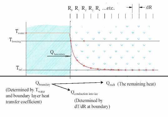
2.4 The figure illustrates the heat transfer procedure that asymptotically

approaches the far-field ice temperature. . . . . . . . . . . . . . . . . . 14

2.5 The hole diameter as a function of time for a range of depths. The drill

strategy delivers a hole of uniform diameter at a required time of 30

hours after the drilling is completed. . . . . . . . . . . . . . . . . . . . 17

2.6 Thisfiguresummarizestheevolutionoftheholesize. . . . . . . . . . . 18

2.7 This figure summarizes the evolution of the hole diameter as a function

of time. The drill strategy delivers a hole of uniform diameter at a

required time of 30 hours after the drilling is completed. . . . . . . . . 19

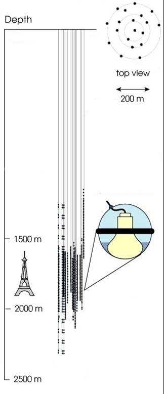
3.1 The figure shows the layout of the AMANDA detector. The top view

shows 19 strings that were deployed. AMANDA detector is roughly

200mwideand500mlong . . . . . . . . . . . . . . . . . . . . . . . . . 25

---

ix

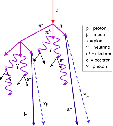
3.2 The figure schemtically shows the interaction of the primary cosmic ray

proton with the atmosphere and the formation of several particles as

the shower evolves. (Image credit: Milagro) . . . . . . . . . . . . . . . 27

3.3 Prompt atmospheric neutrinos are predicted to follow a harder spec-

trum than conventional atmospheric neutrinos. The flux of prompt

atmospheric neutrinos is highly uncertain and predictions range over

several orders of magnitude. Image Credit: Jessica Hodges . . . . . . . 30

3.4 The distribution of lateral separation from shower core for the DPMJET-

II for charm and coventional muons in each event with the first inter-

action and multiple interactions isolated. . . . . . . . . . . . . . . . . . 33

3.5 The total energy distribution for the DPMJET-II for charm and con-

ventional muons for each event with first interaction and multiple in-

teractionsisolated. . . . . . . . . . . . . . . . . . . . . . . . . . . . . . 34

5.1 The angular distribution of atmospheric muons in AMANDA-II at a

depth of 1730m using the MAM ice model with the SYBILL interaction

model and the 2001 experimental data. . . . . . . . . . . . . . . . . . . 45

5.2 The depth-intensity of atmospheric muons in AMANDA-II using the

MAM ice model and the SYBILL interaction model with the 2001 ex-

perimentaldata.. . . . . . . . . . . . . . . . . . . . . . . . . . . . . . . 46

5.3 The relative difference between MAM SYBILL Monte Carlo and AMANDA-

II 2001 data as a function of depth. . . . . . . . . . . . . . . . . . . . . 47

5.4 The relative difference between MAM SYBILL Monte Carlo and AMANDA-

IIexperimentaldataasafunctionofzenithangle. . . . . . . . . . . . . 47

---

x

5.5 The angular distribution of atmospheric muons in AMANDA-II at a

depth of 1730m using the Millenium ice model with the SYBILL inter-

action model and the 2005 experimental data. . . . . . . . . . . . . . . 48

5.6 The depth-intensity of atmospheric muons in AMANDA-II using the

Millenium ice model and the SYBILL interaction model with the 2005

experimentaldata. . . . . . . . . . . . . . . . . . . . . . . . . . . . . . 48

5.7 The relative difference between Millenium SYBILL Monte Carlo and

AMANDA-II 2005 experimental data as a function of depth. . . . . . . 49

5.8 The relative difference between Millenium SYBILL Monte Carlo and

AMANDA-II 2005 experimental data as a function of zenith angle. . . 49

5.9 The zenith angle difference between the reconstructed and true zenith

angle known from simulation is plotted on x-axis while normalized

counts are plotted on y-axis. The respective slices in zenith are indi-

cated in the plot. Red is before quality cuts while blue is after quality

cuts. From left to right and top to bottom there are 10 slices shown

that go from0.0-0.5 in increments of 0.05. . . . . . . . . . . . . . . . . 52

5.10 The zenith angle difference between the reconstructed and true zenith

angle known from simulation is plotted on x-axis while normalized

counts are plotted on y-axis. The respective slices in zenith are indi-

cated in the plot. Red is before quality cuts while blue is after quality

cuts. From left to right and top to bottom there are 10 slices shown

that go from0.5-1.0 in increments of 0.05. . . . . . . . . . . . . . . . . 53

---

xi

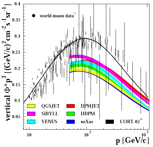
5.11 Comparison of CORSIKA vertical muon flux for various interaction

models. . . . . . . . . . . . . . . . . . . . . . . . . . . . . . . . . . . . 54

6.1 The N

ch

variation for the DPMJET-II for signal and background (at the

final level after event selection criteria are implemented) when spectral

index is varied by

±0.02

shown as a ratio. . . . . . . . . . . . . . . . . 60

6.2 The N

ch

distribution for the DPMJET-II for signal and background

(at the final level after event selection criteria are implemented) when

spectralindexisvariedby±0.02shownasaratio.. . . . . . . . . . . . 60

6.3 The N

ch

variation for the DPMJET-II for background (at the final level

after event selection criteria are implemented) when compared with an

equally weighted simulation of SYBILL and DPMJET-II is shown. . . . 61

6.4 The N

ch

distribution for the DPMJET-II for background (at the final

level after event selection criteria are implemented) when compared

with an equally weighted simulation of SYBILL and DPMJET-II is

shown. . . . . . . . . . . . . . . . . . . . . . . . . . . . . . . . . . . . . 61

6.5 The N

ch

variation for the DPMJET-II millenium ice model (at the

final level after event selection criteria are implemented) when com-

pared with an equally weighted simulation of DPMJET-II millenium

and DPMJET-II AHA model is shown. . . . . . . . . . . . . . . . . . . 62

6.6 The N

ch

distribution for the DPMJET-II millenium ice model (at the

final level after event selection criteria are implemented) when com-

pared with an equally weighted simulation of DPMJET-II millenium

and DPMJET-II AHA model is shown. . . . . . . . . . . . . . . . . . . 62

---

xii

7.1 Energy fraction distributions using various models for charmed baryon

and mesons for energies of 10, 10

2

, 10

3

, and 10

4

TeV . . . . . . . . . . 73

7.2 The mean multiplicity and the Z-moments of pions and kaons as a

function of primary energy. The top ensemble of points denote pions

while the bottom ones denote kaons . . . . . . . . . . . . . . . . . . . . 74

7.3 The trasverse momentum, longitudinal momentum and lateral separa-

tion of the secondary particles produced by air showers for a 1 PeV

monoenergetic beam of primary protons at a fixed zenith angle of 65

degrees. . . . . . . . . . . . . . . . . . . . . . . . . . . . . . . . . . . . 74

7.4 Shows the average number of muons produced per event as a function

the lateral separation from the shower core at surface of earth for show-

ers initiated by the full cosmic ray spectrum, full cosmic ray spectrum

for zenith>80 degrees, for primaries in the energy range of 1-1000 PeV

and monoenergetic primary energy of 1 PeV with no showering (only

the first interaction) and after the full shower develops (multiple inter-

actions) with events containing atleast 1 prompt muon (produced from

a charmed particle) tagged as “PROMPTS” and for no prompt muon

involved as “CONV”. All data has been normalized to 1 years worth

lifetime. . . . . . . . . . . . . . . . . . . . . . . . . . . . . . . . . . . . 75

---

xiii

7.5 Shows the average number of muons produced per event as a function

the lateral separation from the shower core at surface of earth for show-

ers initiated by the full cosmic ray spectrum, full cosmic ray spectrum

for zenith>80 degrees, for primaries in the energy range of 1-1000 PeV

and monoenergetic primary energy of 1 PeV after the full shower devel-

ops (multiple interactions) with showers produced by protons and iron

identified separately. All data has been normalized to 1 years worth

lifetime. . . . . . . . . . . . . . . . . . . . . . . . . . . . . . . . . . . . 76

7.6 Shows the average number of muons produced per event as a func-

tion the lateral separation from the most energetic muon at surface of

earth for showers initiated by the full cosmic ray spectrum, full cosmic

ray spectrum for zenith>80 degrees, for primaries in the energy range

of 1-1000 PeV and monoenergetic primary energy of 1 PeV with no

showering (only the first interaction) and after the full shower develops

(multiple interactions) withevents containing atleast 1 prompt muon

(produced from a charmed particle) tagged as “PROMPTS” and for no

prompt muon involved as “CONV”. All data is normalized to 1 years

worthlifetime . . . . . . . . . . . . . . . . . . . . . . . . . . . . . . . . 77

---

xiv

7.7 Shows the average number of muons produced per event as a function

the lateral separation from the most energetic muon at surface of earth

for showers initiated by the full cosmic ray spectrum, full cosmic ray

spectrum for zenith>80 degrees, for primaries in the energy range of

1-1000 PeV and monoenergetic primary energy of 1 PeV after the full

shower develops (multiple interactions) with showers produced by pro-

tons and iron identified separately. All data is normalized to 1 years

worthlifetime . . . . . . . . . . . . . . . . . . . . . . . . . . . . . . . . 78

7.8 Shows the average number of muons produced per event as a function

the lateral separation from the most energetic muon at detector for

showers initiated by the full cosmic ray spectrum, full cosmic ray spec-

trum for zenith>80 degrees, for primaries in the energy range of 1-1000

PeV and monoenergetic primary energy of 1 PeV with no showering

(only the first interaction) and after the full shower develops (multiple

interactions) with events containing atleast 1 prompt muon (produced

from a charmed particle) tagged as “PROMPTS” and for no prompt

muon involved as “CONV”. All data is normalized to 1 years worth

lifetime. . . . . . . . . . . . . . . . . . . . . . . . . . . . . . . . . . . . 79

---

xv

7.9 Shows the average number of muons produced per event as a function

the lateral separation from the most energetic muon at detector for

showers initiated by the full cosmic ray spectrum, full cosmic ray spec-

trum for zenith>80 degrees, for primaries in the energy range of 1-1000

PeV and monoenergetic primary energy of 1 PeV after the full shower

develops (multiple interactions) with showers produced by protons and

iron identified separately. All data is normalized to 1 years worth lifetime 80

7.10 Shows the sum total of surface energy of all the muons in an event for

showers initiated by the full cosmic ray spectrum, full cosmic ray spec-

trum for zenith>80 degrees, for primaries in the energy range of 1-1000

PeV and monoenergetic primary energy of 1 PeV with no showering

(only the first interaction) and after the full shower develops (multiple

interactions) with events containing atleast 1 prompt muon (produced

from a charmed particle) tagged as “PROMPTS” and for no prompt

muon involved as “CONV”. All data is normalized to 1 years worth

lifetime. . . . . . . . . . . . . . . . . . . . . . . . . . . . . . . . . . . . 81

---

xvi

7.11 Shows the sum total of energy of all the muons in an event at the

detector for showers initiated by the full cosmic ray spectrum, full cos-

mic ray spectrum for zenith>80 degrees, for primaries in the energy

range of 1-1000 PeV and monoenergetic primary energy of 1 PeV with

no showering (only the first interaction) after the full shower develops

(multiple interactions) with events containing atleast one prompt muon

(produced from a charmed particle) tagged as “PROMPTS” and for no

prompt muon involved as “CONV”. All data is normalized to 1 years

worthlifetime . . . . . . . . . . . . . . . . . . . . . . . . . . . . . . . . 82

7.12 Shows the zenith angle distribution of showers initiated by the full cos-

mic ray spectrum, full cosmic ray spectrum for zenith>80 degrees, for

primaries in the energy range of 1-1000 PeV and monoenergetic primary

energy of 1 PeV with no showering (only the first interaction) and after

the full shower develops (multiple interactions) with events containing

atleast 1 prompt muon (produced from a charmed particle) tagged as

“PROMPTS” and for no prompt muon involved as “CONV”. All data

is normalized to 1 years worth lifetime . . . . . . . . . . . . . . . . . . 83

8.1 The minimized value of chisquare is shown for different levels of signal. 89

8.2 The elliptical contours of chisquare for the fraction of Millenium and

AHA backgrounds are shown forcing the signal contribution to be zero

while making a fit to the data. . . . . . . . . . . . . . . . . . . . . . . . 89

---

xvii

8.3 The elliptical contours of chisquare for the fraction of Millenium and

AHA backgrounds are shown for best fit value of signal while making a

fittothedata.. . . . . . . . . . . . . . . . . . . . . . . . . . . . . . . . 90

8.4 The elliptical contours of chisquare for the fraction of Millenium and

AHA backgrounds are shown for the allowed level of signal at 90%

confidence level while making a fit to the data. . . . . . . . . . . . . . . 90

8.5 The signal and background spectra for the AHA and Millenium models

together with the minimum bias experimental data before fitting are

shown. . . . . . . . . . . . . . . . . . . . . . . . . . . . . . . . . . . . . 91

8.6 The scaled levels at the best fit values of signal and background spec-

tra for the AHA and Millenium models are shown together with the

minimum bias experimental data. . . . . . . . . . . . . . . . . . . . . . 91

---

1

Chapter 1

Introduction

The Antarctic Muon and Neutrino Detector Array (AMANDA) is designed to detect

high energy neutrinos using the three kilometer thick ice cap covering the South Pole.

AMANDA in its design consists of a large array of phototubes located under the ice.

This array of phototubes embedded in the icecap at depths of 1500 to 2000m captures

the Cherenkov radiation from the ultra relativistic charged leptons that are produced

when neutrinos undergo charged current interactions with nucleons in the ice.

The main aim of AMANDA is to detect extra-terrestrial neutrinos. The back-

ground to the observation of these neutrinos is the flux of atmospheric muons and

neutrinos produced in cosmic ray showers in the atmosphere. Atmospheric muons can

reach the detector only from above, because the range of muons in earth is only a

few kilometers. Atmospheric muons are therefore only downgoing and these can be

easily filtered out by using the earth as a filter and looking at upward-moving neutri-

nos produced in the northern hemisphere. Atmospheric neutrinos can instead reach

the detector from all directions. Hence they are an irreducible background for diffuse

astrophysical neutrino fluxes. It is very important to evaluate their intensity with

reasonable accuracy.

---

2

At GeV energies the atmospheric fluxes are dominated by the decays of relatively

long-lived particles such as π

±

and K

±

mesons. With increasing energy, the probability

increases that such particles interact in the atmosphere before decaying. This implies

that even a small fraction of short-lived charmed particles can give the dominant

contribution to high energy muon and neutrino fluxes. These “prompt” muons and

neutrinos arise through semi-leptonic decays of hadrons containing heavy quarks, most

notably charm. Estimates of the magnitude of the prompt atmospheric fluxes differ by

almost two orders of magnitude making the significance of evaluating their intensity

very important.

The main principle in this thesis is that it is possible to overcome the theoretical

uncertainty in the magnitude of the prompt neutrino fluxes by deriving their intensity

from a measurement of the down-going prompt muon flux. The suggestion is based

on the observation that due to the charmed particle decay kinematics for the semi-

leptonic decays into neutrino and muon fluxes, the prompt muon and neutrino flux

are essentially the same at sea level. Importantly, this result is independent of the

charm production model. It should be stressed that down-going prompt muons and

not up-going neutrino induced muons are used to get limits on the prompt neutrino

flux. Prompt muons are easy to detect and there are ways of separating them from

the conventional muons using different zenith angle and energy spectral shapes.

This analysis of the atmospheric charm component is challenging for the fact that

there are no robust simulations for producing atmospheric prompt muons. Further,

the limited angular and energy resolutions of AMANDA combined with the lack of

availabilty of a model makes life very hard for a researcher.

---

3

Studies were also done on the introduction of theoretical models used to calculate

the heat transfer and refreezing rates in boreholes in cold ice at the south pole and

a comparison of these results with experimental data from the AMANDA holes. The

calculations are based on models derived for phase change with a moving boundary

layer in cylindrical coordinates. This work improved estimates of fuel consumption

and contributed to a better efficiency in the drilling of holes for project IceCube.

---

4

Chapter 2

Strategies to optimize the hotwater

drilling method for IceCube

During the 1990s 23 holes were drilled to depths ranging from 1000 to 2450 meters

at the South Pole to build the AMANDA neutrino telescope. A large hot water drill

was used to drill the holes. This technique was chosen because it was the only one

conceivable to meet the requirements to produce 60cm diameter holes filled with water.

Pioneering efforts to 1000 m depth were successful and allowed the installation of the

first optical sensors in polar ice at the South Pole. The drill grew in size as depth

and hole diameter requirements increased until it reached a maximum thermal power

of 2.2 MW. It became clear that this drill would not be adequate to drill to depths

of 2450 meters, required for IceCube. At depths below 2000 meters drilling became

slow and inefficient. The next generation IceCube detector would require drilling 80

holes in a five year period. A new enhanced hot water drill (EHWD) with a power

of about 5 MW would need to be designed to drill two holes per week. The following

study was initiated to optimize the drill design and drilling strategy and confirm

relatively rough estimates on fuel consumption. We developed a model that allowed

---

5

us to calculate a drilling procedure that will result in a hole diameter large enough

to ensure successful deployment of detector strings with acceptable fuel requirements.

The model suggests drilling and reaming rates based on heat input that will provide

an optimum hole diameter profile. The result is a barrel shaped hole that compensates

for different freezing rates that are a function of ice temperature and time of exposure

to heat. The calculations and predictions are verified from simulations with drill data

from the AMANDA holes. The robustness of the calculation is checked by applying

perturbations to critical system parameters.

IceCube is a one-cubic-kilometer international high-energy neutrino observatory

being installed in the clear deep ice at the South Pole. It will open unexplored bands

for astronomy, including the PeV energy region, where the Universe is opaque to

high-energy gamma rays originating from beyond the edge of our own galaxy, and

where cosmic rays do not carry directional information because of their deflection

by magnetic fields. The detector will consist of 80 strings of optical modules placed

between 1450 and 2450 meters depth. This depth range takes advantage of the clear

ice below the bubbly ice region and avoids the shear layer between the bottom of

the ice and the detector. The holes will have a diameter of approximately 60 cm to

support the installation of the optical module strings, which are 43 cm in diameter.

The additional size is required to compensate for freezing that takes place on the hole

walls after drilling and during deployment. Hot water drills operate by pumping water

that has been heated under high pressure to a drill head where the hot water jet is used

to melt the ice. In impermeable ice, the hole is filled with water, which is recycled to

the surface by a submersible pump. The water is then reheated and pumped through

---

6

the drill head to melt more ice. Approximately 8% of the ice volume must be replaced

by water from the surface to make up for the volume lost in the phase change. Before

the AMANDA project these drills were generally portable and limited to less than 1500

meters in depth and to smaller diameters. The cold

?

50

◦

C ice at Sthe South Pole,

depth requirement of 2400m and hole diameter of 60 cm required a much larger drill.

The drill used for AMANDA evolved over the life of the project and grew from 1.6

to 2.2 MW maximum heat input. The drill was pressure limited to 1000 psi operating

pressure, which limited flow as lengths of hose were added. At depths beyond 2000

meters the drill became increasingly inefficient. Fuel consumption per hole was over

10000 gallons and the time required to drill a 2400 meter hole was well over 100 hours,

in one case more than 150 hours. Neither of these figures was acceptable for the 80

holes required for IceCube. A new drill design was proposed that would provide a

constant heat input of about 5MW over the entire drilling depth. A larger hose was

needed to accommodate the higher flow and the hose was to be housed on a single

large reel. Single point power generation, with heat scavenging, have replaced ancient

generators and diesel driven pumps to improve efficiency. In addition the entire drill

heating and pumping plant have been placed in mobile drilling structures that reduce

set up and build down time. The goal is to drill up to 18 holes per year, completing

2 holes per week. The 40 hour drilling time per hole drives the heat input. Since the

drills have all been equipped with calipers and navigation packages, it is possible to

create a map of the hole including a diameter vs depth curve. These measurements

and curves are required to assure the hole diameter remains large enough to permit

the deployment of the optical modules over a 30-hour period after drilling ceases.

---

7

Crude models were constructed during the AMANDA project to predict the amount

of freezing that would occur during this period. This paper is an introduction to the

theoretical models used to calculate the heat transfer and refreezing rates in boreholes

in cold ice and to compare the results with experimental data from the AMANDA

holes. The calculations are based on models derived for phase change with a moving

boundary layer in cylindrical coordinates.

2.1 Description of the thermal process

A large hot water drilling system consists typically of the following main com-

ponents.

•

High-pressure pumps to pump the water to the drill head.

•

Heaters to heat the water to near boiling.

•

Drill hose to deliver the water to the drill.

•

Drill head and nozzle to direct water to the front to warm and melt ice.

•

A return submersible pump to recycle cold water from the bore-hole.

The surface components consist of high-pressure pumps and a heating plant. Heat

losses from this part of the system are low compared of the total heat budget in large

drill systems because the hoses are well insulated. The hose hangs vertically in the

hole, which is filled with water below a depth of 50m. A parcel of water moving

through the hose loses heat to the surrounding water through conduction across the

hose wall and convection to the surrounding water, which is moving slowly up the

hole. The advective term is ignored in these calculations. It is desirable to move the

---

8

14

13

15

17

16

7

8

7

1

2

2

5

6

10

10

10

10

3

4

9

0

9a

Ic e Cub e

Drill Site La yo ut

Hea ting

S tri ng Deployment

Drill Control

Tanks

Ge ne rators

Pre-Hea t

Tanks

Pumps

Water

Well

Parts storage

work area

7/1 3/0 0

S witching

gear

12

11

Hot-Water Drilling

Figure 2.1: The figure describes the schematic view of the IceCube En-

hanced Hot Water Drill (EHWD) at the surface.

water through the hose as rapidly as possible to keep the residence time in the hose

to a minimum. The amount of heat available at the nozzle drops exponentially with a

decay length λ of the hose where the heat available has fallen to half of that available

at the surface. The decay length depends on the conductivity of the hose material, the

hose wall thickness and the velocity of fluid through the hose. Heat lost through the

hose helps keep the hole from refreezing. Later we will discuss how the decay length

influences drilling and reaming efficiency.

The hot water drill head consists of a massive steel pipe to keep the drill plumb,

and a housing for the electronics and navigation package. A nozzle is designed to

accelerate the speed of the water while keeping the flow intact to create turbulence

ahead of the drill. In cold ice as at South Pole the ice must first be warmed before

---

9

Figure 2.2: Depth dependnce of the temperature of South Pole Ice.

it can be melted. This can limit drilling speed if the narrow portion of the drill is

short or the velocity at the nozzle is low. A temperature profile of the ice at the South

Pole is shown in figure 2.2. The heat provided by the injected hot water of about 800

liters/min is not dissipated immediately. Energy remains in the form of hot water that

continues to warm and melt the surrounding ice. Some of the energy is conducted into

the surrounding ice. The result is a long plume of warm water that gradually melts

the hole wall to a larger diameter with time. With large hot water drills such as the

AMANDA or IceCube drill this plume can extend more than 100 meters behind the

drill.

As the return flow drifts back up, the cold water column is slightly heated by

losses from the hose. These losses slow the refreezing rate. The effects will be discussed

in a later section. Water at the top of the hole having a temperature of 2

◦

C is recycled

using a submersible pump.

---

10

Figure 2.3: Schematic view of the hotwater drilling method.

At the surface water is pumped through heaters into the high-pressure hose,

which transports the energy into the borehole where it is used for melting the ice. The

heat input to the borehole is determined from the flux and temperature of pumped

water. The hose at the surface is usually well insulated and the water typically loses

only 2-3

◦

C from the point on the surface where it is pumped until it reaches the top

of the borehole.

A hot water packet takes several minutes travel down the hose to the drill tip,

so an imperfectly insulated hose conducts heat to the surrounding borehole which is

typically filled with cold water. The hose and cable tension is monitored to ensure that

the drill tip does not touch the bottom of the hole. A parcel of fluid traveling down the

hose can be said to lose heat only through the walls of the hose, since the temperature

gradients along the direction of flow are negligible as compared to the radial gradients.

---

11

These hose losses slow down the process of refreezing that occurs at the top of the hole

and cannot be regarded as a waste. Because of the exponential decay of temperature

and consequently the power available, it is important to maximize the flow within

the pressure capability of the hose. For the EHWD the thermal conductivity of the

hose is 0.4W/m-K [2] and the flow rate is 200 gallons/minute and thus λ is around

8000m. There would also be an advective term, which comes from the conductivity of

the water that fills the hole. In the problem we shall neglect advective heat transfer,

which would fluctuate as the hole size changes. In the past, water was heated to

90

◦

C, losing heat as it travels from the heating plant to the surface of the hole. The

calculations that follow were done with a surface temperature of 88

◦

C, which can be

obtained by suitably insulating the hose from the heaters to the hole opening without

much heat lost into the surrounding atmosphere.

2.2 Methodology and Assumptions

Symmetry allows for an assumption of azimuthal independence. We will simplify

the problem to the one along the radial direction alone because the longitudinal gradi-

ents are negligible. As the heat is exchanged across the ice-water boundary refreezing

will occur. The moving boundary of the phase change interface presents special dif-

ficulties for numerical procedures, since the position of the boundary is dependent

upon a varying temperature field in ice. The boundary condition would be that the

temperature of the ice water interface is always at 0

◦

C. At each time step the change

in radius is calculated from the amount of heat that enters the system in the form of

hose losses and the amount of left over heat energy that goes from the hot water that

is left after the initial melting has occurred. The heat left decays exponentially and

---

12

for purposes of our calculation, we assume that this heat continues to melt the ice for

a period of four hours after which it goes down to about 2C when it becomes cold

enough that it can no longer melt ice. However, in this section we will briefly look at

the underlying equations. The problem may be formulated in cylindrical co-ordinates

with the z-axis directed downward from the surface along the axis of the hole. The

system is azimuthally symmetric. We will simplify the problem to one along the radial

direction alone because the longitudinal gradients are negligible.

2.3 Description of the model and assumptions

Here we describe a list of the model assumptions in the calculation:

a) The method used to solve the heat transfer differential equation is a numerical

finite difference method. For this purpose, we modeled the problem with a space mesh

where the grid element was 0.15cm wide (1% of the initial radius). We used 1300

elements to span a total area of 3.6m

2

at each depth. The number of elements in the

grid is chosen in such a way that the solution to the problem converges at each depth

in a reasonable time and with sufficient precision. The number of grid points chosen

was increased until the result didn’t change significantly with increasing resolution.

b) The time resolution for each time step was taken as 0.0001 times the charac-

teristic time of the system, which is the total borehole closure time (100 hours). Each

time the size of the hole changed, the number of grid points inside the boundary were

suitably adjusted, allowing us to locate the point on the ice-water interface.

c) Total heatflow is 200 gal/min of water with a temperature of 88

◦

C at the top

of the borehole. This corresponds to a total power of 4.65MW at the top of the hole.

d) The circulated water loses around 40% of the heat before it travels from the

---

13

nozzle to the widest point of the drill hole (15m above the drill head). This heat is

available for initial melting and for constructing a sufficient diameter hole for the drill

to fit. This process takes 1-2 minutes and is assumed to be non-heat conducting with

regards to the surrounding ice. The temperature to which the water cools during this

instantaneous conduction is given by 54exp(-z/λ), where z is the depth and λ is the

decay length of the hose.

e) Once the initial melting described above is complete, the hot water remains

inside the hole and continues to increase the diameter of the hole, as some of the heat

is lost into its surroundings. This process has been modeled as a typical steady-state

heat conduction problem with a 4-hour duration and an exponential decay function,

where half of the heat decays in the first hour.

f) We modeled the down-hole path as segments of length 100m at constant

temperature. The conditions inside each slice are assumed to be non-varying and

the heat transfer equations are solved inside the mesh surrounding it. Once all the

calculations are done for one slice we move onto the next slice and so on.

g) A final target diameter at 45cm in each of the 100m slices at the end of

operation was set.

h) The thermal properties of ice (specific heat and freezing point) are assumed

to be constant throughout the hole.

i) We obtained the hose losses by dividing the total heat available at any depth

by the λ of the hose. We neglected the conductivity of the water, so all thermal

conductivity is assumed to come from the hose alone. By neglecting the advective

heat transfer, we may have overestimated the hose losses and underestimated the heat

---

14

Figure 2.4: The figure illustrates the heat transfer procedure that asymp-

totically approaches the far-field ice temperature.

available at the bottom of the hole but all these corrections can be neglected to first

order.

j) We model the reams as an instantaneous process in which no heat is conducted

into the surrounding ice and it is entirely used for melting the ice on the borehole walls.

2.4 Optimal drilling algorithm

The drilling strategy is optimized to obtain a hole of constant diameter at some

specified time of typically 35 hours after drilling is completed. The minimum amount

of time that we spend inside the hole subjected to constraints like the target uniform

diameter after deployment being 45 cm and the drill fitting through can be accom-

plished by a simplex minimizer however it can be observed that the solutions to the

problem exhibit monotonic nature and thus we can find the optimum just by moving

in one direction. The final time step to obtain optimum solution is in turn dependent

---

15

on the solutions in each of the slices so there is a need for a first guess solution. We

start out at a high drill speed of 200m/hr and a ream speed of 450m/hr respectively

inside the slice. We calculate the initial diameter that we obtain from the cooling

of water from the nozzle to the drill head. If we don’t get sufficient size of the hole

(initial diameter) for the drill to fit through then we reduce the drill speed by 5m/hr

until the condition of the drill passing through is met. There is a maximum of the

drill speed that we use for our optimization. Once this condition is met we calculate

the position of the ice-water boundary at a time t, the initial guess on total time spent

inside the hole plus the estimated deployment time. If the diameter of the hole is less

than the target diameter of 45cm then we reduce the ream speed in steps of 10m/hr

and check if we reach the target diameter at which point we stop and move onto the

next slice. Once the minimum limit on ream speed (180m/hr) is reached without the

target diameter getting to 45 cm, we reduce the drill speed from the maximum limit

obtained for the drill to fit through in steps of 5m/hr till we get the required target

diameter. Once the required target diameter is established we record the values of the

drill speed and the ream speed used for accomplishing the required target diameter

and calculate the time spent by the drill head in this slice during the drilling and the

reaming operations. Then we move on to the next 100metre slice, the drilling oper-

ation in this slice is delayed by a factor of time that we spent in the previous slices

drilling, in other words it takes time for the drill to get here so we subtract the time

we spent till we get to this slice from our initial guess on total time. This analysis is

repeated in slices of 100 metres until we get to the bottom of the hole. By summing

up the times spent drilling and reaming in each of these slices we get the total time

---

16

spent inside the hole. This should for iterative purposes be close to our initial guess

of 50 hours. If this is lesser (which is usually the case, considering that we start out

with a larger value than what we think our solution is going to be) then we reduce the

initial guess (50 hours) in steps of 1 hour and repeat the entire procedure described

in this section till the iteration is established. Thus the drill speed, ream speed and

other parameters at each depth that satisfy all these conditions are the solutions to

our optimization problem. At these parameter values we get a uniform hole of 45cm in

diameter at all depths and this also minimizes the total time spent by the drill inside

the hole.

2.5 Results

A baseline model assumes the most likely values for the parameters encountered

in the actual field operation. The results of the optimization process are shown in the

following figures. Figure 2.5 illustrates the optimal refreeze process. While the hole is

drilled at different times and the refreeze rates differ with depth they reach an identical

diameter at a predefined target time. This is the time theoretically available for the

deployment team to deploy the string. After this time the hole would be too small

and the string would get stuck and freeze in prematurely. Obviously some contingency

time needs to be taken into account to ensure a safe deployment process.

---

17

0

10

20

30

40

50

60

70

80

0

10

20

30

40

50

60

70

TIME(hrs)

DIAMETER(cm) ,..

0m

600m

1200m

1800m

2300m

Figure 2.5: The hole diameter as a function of time for a range of depths.

The drill strategy delivers a hole of uniform diameter at a required time

of 30 hours after the drilling is completed.

---

18

0

10

20

30

40

50

60

70

80

0

500

1000

1500

2000

2500

Depth(m)

10 hour(amidst drilling)

20 hour

30hour(partly reamed)

40 hour

50 hour

60hour

63 hour(operation end)

Diameter (cm)

Figure 2.6: This figure summarizes the evolution of the hole size.

---

19

-60

-50

-40

-30

-20

-10

0

0

0.2

0.4

0.6

0.8

1

1.2

1.4

1.6

1.8

2

Distance From Centre (m)

10 hours

20 hours

30 hours

40 hours

50 hours

60 hours

Temperatture (Celsius)

Figure 2.7: This figure summarizes the evolution of the hole diameter as

a function of time. The drill strategy delivers a hole of uniform diameter

at a required time of 30 hours after the drilling is completed.

2.6 Robustness of Predictions

The above analysis assumes that the inputs used are known accurately. However,

the inputs could generally vary due to fluctuations during the drilling operation or

simply because they haven’t been accurately determined. So we performed another

analysis in which we allowed a perturbation on one input at a time and checked the

results against our original overall drilling strategy, paying special attention to the

total time we spend inside the hole and our fuel estimates. The decay length, power

available at surface, deployment time and desired target diameter are varied and a

range of outputs corresponding to optimal strategy are quoted in tabular forms.

---

20

λ = 5000m

λ = 8000m

Heat (Surface to 800m) (MW)

5.0

2.2

Heat In (at 2000m) (MW)

5.0

1.9

Heat Out (at 2000m) (MW)

4.0

1.6

Drill Rate (at 2000m) (meters/minute)

1.5

?

2.0

0.5

Flow Rate (at 2000m) (gallons/minute)

200

85

Fuel Consumption (gallons/hour)

200

85

Weight (pounds)

400000

250000

Set-upTime(days)

18? 25

35? 42

Fuel (gallons/hole)

6000? 7000 10000? 12000

Table 2.1: The input parameters that go into the old AMANDA drill (λ

= 5000m) and the new IceCube drill (λ = 8000m) are compared.

λ =

λ =

λ =

5000m 8000m 11000m

Drill Time (hrs)

19.28 19.06 21.17

Ream Time (hrs)

10.67 12.36 13.00

Total Time (hrs)

30.00 31.42 32.55

Total Energy Deposited (GJ)

510

538

549

Energy lost to Surroundings (GJ) 358

386

397

Energy Ratio

0.948 1.00

1.02

Drill Fuel (gal)

3856 3812 4234

Total Fuel (gal)

6000 6284 6550

Table 2.2: The outputs for the optimum strategy and consequently the

fuel consumption are quoted by varying the thermal conductivity of the

hose λ

---

21

20hr deploy 25hr deploy 35hr deploy 40hr deploy

Drill

17.96

17.96

20.52

23.53

Time (hrs)

Ream

9.50

11.29

13.16

13.14

Time (hrs)

Total

27.47

29.25

33.68

36.68

Time (hrs)

Total Energy

465.3

495.6

570.48

621

Deposited (GJ)

Energy lost

313.3

343.6

418.48

469

to Surroundings (GJ)

Energy

0.864

0.921

1.06

1.154

Ratio

Drill

3592

3592

4104

4706

Fuel (gallons)

Total

5494

5850

6736

7336

Fuel (gallons)

Table 2.3: The output parameters corresponding to the optimum strategy

and consequently the fuel consumption are quoted by varying the deploy-

ment time.

---

22

5%

10 %

15 %

20 %

powercut powercut powercut powercut

Drill Time (hrs)

20.93

23.6

26.9

31.25

Ream Time (hrs)

12.90

13.18

13.40

13.63

Total Time (hrs)

33.83

36.78

40.36

44.89

Total Energy Deposited (GJ)

544.3

560

580.6

608.2

Energy lost to Surroundings (GJ) 392.3

408

428.6

456.2

Energy Ratio

1.01

1.04

1.077

1.128

Drill Fuel (gallons)

3977

4248

4573

5000

Total Fuel (gallons)

6437.2

6620

6860

7182.4

Table 2.4: The output parameters corresponding to the optimum strategy

and consequently the fuel consumption are quoted by cutting down the

power available.

Diameter=45cm Diameter=50cm

Drill Time (hrs)

19.06

22.24

Ream Time (hrs)

12.36

13.29

Total Time (hrs)

31.42

35.53

Total Energy Deposited (GJ)

538

601.8

Energy lost to Surroundings (GJ)

386

424.3

Energy Ratio

1.01

1.12

Drill Fuel (gallons)

3812

4448

Total Fuel (gallons)

6284

7106

Table 2.5: The output parameters corresponding to the optimum strategy

and consequently the fuel consumption are quoted by varying the desired

target diameter.

---

23

2.7 Conclusions and Summary

A fundamental analysis of the available drill data and a heat transfer simulation

was performed. Further a thermodynamic analysis of the process of drilling and re-

freeze and compared our results with existing data. This provided a better prediction

of the refreeze rates and an optimal strategy for efficiently drilling uniform holes. We

also infer that it is always better strategy to put energy into the ice as late as possible

to prevent it from refreezing; in other words drill fast and ream slow. This is because

when we put in heat energy late we are fighting less steep temperature gradients in

the surrounding ice. In order to make full use of the analysis we propose a more

regulated system called the smart drill. In this system the computer would regulate

the drill speed in such a way that the borehole diameter is uniform and of the size as

predicted by an optimized freeze back prediction. Studying the system perturbations

on a one at a time basis gave us valuable insights into the development of such a

system. A significant improvement in hole quality and fuel consumption will be to the

benefit of the proposed IceCube project. The modifications suggested in this analysis

contributed to a significant reduction of the fuel consumption for the IceCube holes

that have been drilled to date (40 holes as of 2008).

---

24

Chapter 3

Measuring the Prompt Atmospheric

Neutrino Flux with Downgoing Muons in

AMANDA-II

3.1 AMANDA Detector

The AMANDA-II detector, Antarctic Muon and Neutrino Detesctor Array, is

located at the South Pole. It consists of a total of 677 optical modules. Each module

comprises of photomultiplier tube and the hardware inside a glass pressure sphere.

These optical modules are attached to 19 strings frozen into the ice, these sensors

are deployed across a range of depths from 1500m to 2000m in a cylinder of 100 m

radius. These modules detect Cherenkov light from secondary charged particles that

are produced from the interaction of a neutrino with ice. AMANDA is integrated

into IceCube detector which is still under construction. IceCube will consist of 70-80

detector strings, each with 60 optical modules. Currently 40 strings are deployed and

are taking data.

---

25

Figure 3.1: The figure shows the layout of the AMANDA detector. The

top view shows 19 strings that were deployed. AMANDA detector is

roughly 200m wide and 500m long

---

26

Detectors like AMANDA-II are sensitive to an energy region in which contribu-

tions from prompt charm decays in cosmic ray showers cannot be neglected and may

constitute an interesting signal as well as a significant background depending on the

nature of the analysis. In searches for diffuse fluxes of astrophysical neutrinos the sig-

nal must be separated at high energies from the background of atmospheric neutrinos.

Atmospheric muons can reach the detector only from above (downgoing through the

earth) because the range of muons in earth is only a few kilometers. Atmospheric

muons are therefore only downgoing. Their flux is typically so high that the region

of sky accessible to even very deep neutrino telescopes is only the hemisphere below

the horizon. Atmospheric neutrinos can instead reach the detector from all directions.

Hence they are an irreducible background for diffuse astrophysical neutrino fluxes. It

is therefore, very important to evaluate their intensity with reasonable accuracy.

3.2 Conventional and Prompt Atmospheric Neutrinos

When cosmic rays interact with the nuclei in the atmosphere there are two types

of particles that are produced that could decay subsequently to give the muon and

neutrino fluxes observed. Once these particles are produced in the atmosphere there

is a competition between interaction and decay. The critical energy at which the

interaction and decay lengths become equal is defined as

ǫ

crit

=

mc

2

cτ

h

o

(3.1)

where mc

2

is the particle’s rest energy, τ the mean life time and the scale constant

h

o

that comes from the assumption of an isothermal atmosphere [36].

---

27

Figure 3.2: The figure schemtically shows the interaction of the primary

cosmic ray proton with the atmosphere and the formation of several par-

ticles as the shower evolves. (Image credit: Milagro)

---

28

Particle ǫ

crit

(GeV)

µ

±

1.0

π

±

115

K

±

850

D

±

3.8×10

7

D

0

,D¯

0

9.6

×10

7

D

±

s

8.5

×10

7

Λ

+

c

2.4

×10

8

Table 3.1: Critical energy for different particles.

Table 3.1 lists the critical energy of parent particles of muons and neutrinos.

These particles could decay and contribute to the atmospheric muon and neutrino

fluxes. As can be seen, this critical energy is very high for charmed particles so

charmed particles decay readily and muons from them are called “prompt” muons.

Above this energy the parent particle is likely to interact or be slowed down before

decaying into a neutrino and muon. Since prompt muons are produced readily they

follow a Φ

∝

E

?

2.7

spectrum resembling the primary cosmic ray spectrum. The π

±

and K

±

mesons decay into conventional neutrinos only if they dont interact in the

atmosphere. If interaction takes place they disappear in the atmosphere and hence

the spectra of conventional neutrinos follows a Φ

∝

E

?

3.7

spectrum.

3.3 Constraining the Prompt Neutrino Flux with the Down-

going Muon Flux

With increasing energy prompt neutrinos become the biggest source of uncer-

tainty in predictions of the atmospheric neutrino flux. The DPMJET-II.55 is the only

model available for simulating prompt muons and it uses a Naumov RQPM model

---

29

[38]. Details of the model are discussed in the next section. As can be seen in figure

3.3 the crossover between conventional neutrinos and the Naumov RQPM model of

charm is between 40 and 200 TeV. The level of prompt neutrinos is a potential problem

which would limit the search for diffuse astrophysical neutrinos at energies above a few

tens of TeV. The suggestion in this thesis is based on the observation that due to the

charmed particle decay kinematics for semi-leptonic decays into muon and neutrino

fluxes these fluxes are essentially the same at sea level. This result is independent of

the charm production model and hence a constraint on a prompt muon flux is equiv-

alent to a constraint on the prompt neutrino flux [31]. There are ways of separating

the prompt muons from the conventional muons in underwater or under-ice detectors,

such as the different zenith angle dependence, the different depth dependence at a

given zenith angle, and the different spectral shape at a given depth and zenith angle

[31].

3.4 Prompt Atmospheric Neutrino Models

The prompt atmospheric neutrino fluxes are uncertain by more than 2 orders

of magnitude. This is because ground-based particle accelerators cannot reach the

energies at which particles are produced in the atmosphere. The uncertainty stems

from the need to extrapolate accelerator data to the high energies probed and the

uncertainities in parameters that go into each model: the primary spectral index, the

critical energy for decay and the Interaction and decay lengths can also play a role.

The Naumov RQPM (Recombination Quark Parton Model) [38, 39] tested in

this thesis is a phenomenological non-perturbative model that takes into account the

contribution of intrinsic charm to the production process. It is assumed that c¯c pairs

---

30

(GeV)]

ν

[E

10

3

4

5

6

7

8

9

]

-1

sr

-1

s

-2

dN/dE [GeV cm

2

-9

-8

-7

-6

-5

-4

10

ν

Conventional atmospheric

ν

Martin GBW prompt atmospheric

ν

Naumov RQPM prompt atmospheric.

ν

CharmC prompt atmospheric

ν

CharmD prompt atmospheric

Figure 3.3: Prompt atmospheric neutrinos are predicted to follow a harder

spectrum than conventional atmospheric neutrinos. The flux of prompt

atmospheric neutrinos is highly uncertain and predictions range over sev-

eral orders of magnitude. Image Credit: Jessica Hodges

---

31

are coupled to a number of constituents in the projectile hadron [40]. The production

of mesons such as π

±

and K

±

in the fragmentation region of proton collisions pro-

ceeds via quark recombination. The evidence for the recombination mechanism comes

from the observation that the longitudinal momentum distribution of the pions in the

fragmentation region of an incident proton is very similar to the distribution of the

valence quarks that they share in the proton, as is revealed in deep inelastic scattering

experiments [44].

3.5 Charm in CORSIKA

CORSIKA is a simulation software package to simulate air showers induced by

primary cosmic rays. The program produces large amounts of data of all the secondary

particles (electromagnetic particles, muons and hadrons). An interaction model is used

to describe the physics of the interactions between cosmic rays and the atmosphere.

The older DPMJET interaction model of CORSIKA produced charmed particles but

they were never allowed to decay so prompt muons could not be simulated. The energy

spectra for prompt muons had to be taken at the surface of the earth from empirical

parametrizations [33] and muons of multiplicity one were simulated because of lack of

prior knowledge of prompt muon multiplicities. In the DPMJET-II-55 framework [20]

charmed particles were treated and hence prompt muons produced subsequently were

tagged through a generation counter based on their parent [16]. For demonstration

purposes the case of first interaction alone was isolated from multiple interactions

in the atmosphere. The plots at the surface of the earth for the energy spectra and

lateral separation from shower axis are shown in figures 3.4 and 3.5 respectively. Figure

3.4 shows that there is not much discrimination power between prompt muons and

---

32

conventional muons when lateral distributions are compared using the DPMJET-II.55

model. This contradicts the hypothesis that prompt muons are single muons as was

previously hypothesized when we didn’t have a prompt muon simulation. DPMJET-

II.55 provided us with a reference model for prompt muons and proved to us that

any strategy to separate prompt muons from conventional muons has to be focused

on using the flatter energy and zenith dependence of prompt muons; if one were to

identify these signal events on top of the background events from conventional muons.

An important part of being able to do a prompt muon analysis using the DPMJET-

II.55 interaction model of CORSIKA is being able to identify them. If one is interested

in muons which come from a decay of ordinary mesons generated in the first interac-

tion, CORSIKA is run and the particle file is scanned for those muons which come

from the first interaction by looking for the generation counter. In CORSIKA the

generation counter is available that tracks the parents of the particles produced. For

instance, for the decays from pions the counter is augmented by 51, for charmed parti-

cles it is 31 to get a discrimination against all other muons. The tagging could also be

used to identify the muons from first interaction using the number on the generation

counter during the production. If an event contains one or more muons that have

their parent as a charmed particle we identify them as prompt muons. A need to tag

the prompt muon events was accomplished this way.

An important part of being able to do a prompt muon analysis using the DPMJET-

II.55 interaction model of CORSIKA is being able to identify them. If one is intrested

in muons which come from a decay of ordinary mesons generated in the first interac-

tion, CORSIKA is run and the particle file is scanned for those muons which come

---

33

Lateral Separation Plot(all tracks)

FIRST INT ONLY(PROMPTS)

FIRST INT ONLY(CONV)

AFTER MULTIPLE INTER(PROMPTS)

AFTER MULTIPLE INTER(CONV)

Lateral Separation(metres) at Surface Of Earth

Percentage of Events in Bin

10

-4

10

-3

10

-2

10

-1

1

0

25

50

75

100

125

150

175

200

225

250

Figure 3.4: The distribution of lateral separation from shower core for the

DPMJET-II for charm and coventional muons in each event with the first

interaction and multiple interactions isolated.

---

34

Muon Energy Plot

FIRST INT ONLY(PROMPTS)

FIRST INT ONLY(CONV)

AFTER MULTIPLE INTER(PROMPTS)

AFTER MULTIPLE INTER(CONV)

log10(Total Muon Energy)GeV at Surface Of Earth

Percentage of Events in Bin

10

-4

10

-3

10

-2

10

-1

1

3

3.5

4

4.5

5

5.5

6

Figure 3.5: The total energy distribution for the DPMJET-II for charm

and conventional muons for each event with first interaction and multiple

interactions isolated.

---

35

from the first interaction by looking for the generation counter. In CORSIKA the

generation counter is available that tracks the parents of the particles produced. For

instance, for the decays from pions the counter is augmented by 51, for charmed parti-

cles it is 31 to get a discrimination against all other muons. The tagging could also be

used to identify the muons from first interaction using the number on the generation

counter during the production. If an event contains one or more muons that have

their parent as a charmed particle we identify them as prompt muons. A need to tag

the Prompt muon events was accomplished this way.

---

36

Chapter 4

Data streams and quality cuts on the 2005

Sample

4.1 First guess reconstructions, livetime and triggers

Likelihood reconstructions need a first guess for the muon track direction to be

able to iterate through and get the final direction. The criteria for designing a first

guess algorithm should be to have fast computing time while approximating the track

direction. Two popular first guess algorithms are described below.

4.1.1 Direct Walk Reconstruction

Direct Walk is a pattern recognition algorithm. The basic algorithm reconstructs

the track direction using only direct hits(hits unscattered in ice).

4.1.2 JAMS Reconstruction

JAMS (Just Another Muon Search) is a pattern recognition algorithm. The basic

algorithm for JAMS creates hit selections and stores an event. A fast algorithm to

find first guess candidate tracks is implemented using hit clusters and these are stored.

---

37

The first guess candidates are narrowed down into a few viable track solutions. One or

two of these best track fits are stored in the event. The quality of the fit is measured

by variable σ

ψ

and in this analysis is set to be less than 0.05. It measures the deviation

of hit clusters from a single track hypothesis.

During the 2005 data run, 1.85 billion events were recorded by AMANDA-II. The

livetime for the 2005 filtered data is 199.25 days. The 2005 data filtering is different

from earlier years in two aspects [19].

1. Modified cross talk is applied.

2. JAMS and Direct Walk at level 1 and level 2 cuts are swapped

The discussion in this chapter is confined to the analysis of downgoing muons.

The output streams relevant to our analysis are the high quality stream and the

minimum bias stream.

4.1.3 High quality stream

Downgoing muon events near the horizon with a high quality in JAMS recon-

struction were selected. Every event with a zenith angle greater then 55 degrees in

JAMS reconstruction fit with a low number for the spread σ

ψ

< 0.05 of its JAMS fit

solutions was identified in this stream.

4.1.4 Minimum bias stream

Every 100th event regardless of how it was triggered was included in this stream.

---

38

4.2 Reconstruction Methods

An arrival timing based likelihood approach as described by the Pandel function

[13] was used to reconstruct the 2005 experimental data and simulation. This function

was subsequently modified for PMT jitter and and a convoluted pandel probability

distribution function was used for this analysis.

4.3 Techniques to Further Improve Background Rejection

Several other techniques were used to improve background rejection. Methods

were also employed to remove electronic crosstalk and other fake events. The quality

of the JAMS fit was checked to ensure high quality events

4.4 Event Simulation and Reweighting

This analysis relied on simulated data sets of background and signal events. The

downgoing conventional atmospheric muons were simulated using the DPMJET-II.55

and SYBILL interaction models. For this work, a preliminary version of CORSIKA

in which the charmed particle decays are enabled in DPMJET-II.55 [20] was used for

signal simulation. Further, we know that the threshold primary energy for muons at

large zenith angles to make it to the detector is high so we do the simulation in two

stages to get enhanced statistics at large zenith angles.

1. Primary threshold energy of 800 GeV of primary cosmic ray energy for muons

between 0 to 70 degrees zenith angle.

2. Primary threshold energy of 10 TeV for primary cosmic ray between 70 to 90

degrees zenith angle.

---

39

The events were simulated with a Φ

∝

E

?

1.7

primary energy spectrum, one power

harder than the spectrum present in nature. The advantage of this approach is that

it reduces the simulation time. The generated events must then be reweighted to the

original cosmic ray spectrum with appropriate normalization factor applied [17].

4.4.1 Preparation of Simulated Events

It would be a huge demand on computer time to simulate the same number of

days livetime worth of simulation as actual experimental data. Simulation is thus

generated with a flatter spectra and event weights are used to reweight to the spectra

we wish to simulate [18]. The simulation events were scaled to match the livetime of

the data during a particular period or year. The simulated events underwent the same

reconstruction procedures as the data and had to satisfy the same zenith angle and

energy requirements. The reconstructed muons deviate from their actual direction due

to mis-reconstruction and we use quality criteria to improve the angular resolution.

---

40

Chapter 5

Response of AMANDA-II to Cosmic Ray

Muons

The flux of downgoing muons detected by the AMANDA-II neutrino telescope is

used as a test beam to check the experimental systematic error and to improve the

knowledge of its response. This work shows the outcome of the effort for a better

understanding of AMANDA-II performance, an improved data filter and event recon-

struction. The simulated predictions for preliminary experimental downgoing muon

angular and depth intensities are compared with experimental results and theoretical

calculations. This report encompasses large statistics of simulated data generated at

large zenith angles using the QGSJET interaction model with a live time of 30 days

and compared to a 30 day span of experimental data for the year 2001. This was

aimed to minimize the effect of statistical and systematic errors on the angular and

depth intensities (particularly close to the horizon). The use of a new Convoluted

Pandel likelihood function ensures improved event reconstruction and stability. This

also ensures good agreement between simulated and experimental data. Further, anal-

ysis was also done using the 2005 experimental data and 2005 simulation using the

---

41

SYBILL interaction model. CORSIKA air shower generator was used to simulate the

interaction of the cosmic rays with the atmosphere.

5.1 Analysis

In order to measure the atmospheric muon angular distribution it is necessary

to evaluate the event trigger and reconstruction efficiencies as a function of the zenith

angle. This requires a Monte Carlo with the complete simulation chain from the pri-

mary interaction in the atmosphere to the detector response based on best knowledge

of the physical processes involved. The event generation is done using CORSIKA

v6.020 with the QGSJET01 interaction model. The model incorporates the curvature

of the earth and the south pole average atmospheric profile. A multi-component pri-

mary cosmic ray energy spectrum [5] is used to get the composition. The generated

muons are propagated to the earth’s surface and then through the ice, considering all

pertinent energy losses. The muons passing through AMANDA-II or near it are folded

into the detector trigger simulation. At this stage the detector response is completely

simulated in order to reproduce the experimentally detected events. This is based on

our overall understanding of the physics and the detector.

The event reconstruction chain for simulation is identical to the one used for

the experimental data. A cleaning procedure then removes the optical modules that

are dead or have odd transient behavior. A time calibration which also accounts

for the signal propagation time through the cables is then employed. A Convoluted

Pandel probability distribution function (a time likelihood based reconstruction) is

used. This accounts for the finite photo-multiplier tube timing resolution of the pulse

obtained when a photon emitted by the muon passes through it. Due to the limited

---

42

angular resolution of the reconstruction, additional cuts are used to improve the event

sample quality for both the experimental and simulated data. These cuts improve the

resolution of the zenith angle and the space angle. .

Tables 5.1 and 5.2 summarize the mean, median, RMS and the extreme tail

of the zenith angle and the space angle resolution. We misreconstruct events closer

to the horizon and this becomes more prominent as we get closer to the horizon.

This can partially be explained by the fact that vertical muons would have larger

track length and larger number of direct hits (hits that are minimally scattered in the

ice before being detected by a optical module) and hence their direction determined

more accurately than a horizontal event. With this resolution we can derive the

experimental angular distribution at AMANDA-II depth by merely calculating the

detector acceptance at each zenith angle bin using the simulated detector response

to unfold the measured data, neglecting the inter-bin correlations. When we neglect

interbin correlations, for each bin in cosine of the zenith angle, the ratio of the true

events generated (that trigger AMANDA) to the reconstructed events (accounting for

various efficiencies during reconstruction) for both the Monte Carlo simulation (known

ratio) and the corresponding experimental data (unknown ratio) can be equated. With

interbin correlations, one needs to account for leakages across bins due to finite angular

resolution and event quality. Neglecting inter-bin correlations can be justified by

demonstrating that these correlations are minimal. We accomplish this by making our

best event quality selections on a sample of 30 days of simulation data. The quality

cuts chosen for this purpose are chi square for the reconstructed track less than 7.3,

track length greater than 120 meters(-15ns to 75ns direct hits only), absolute value of

---

43

the the difference between the zenith angle reconstructed using odd hits only and using

even hits only from hits ordered. Further these inter-bin overlaps can be minimized

by increasing or decreasing the bin size in cosine zenith. The bin-size for the actual

intensity distribution is defined at twice the RMS value of statistics shown in tables

5.1 and 5.2 so that most events are self contained and overlaps are minimal. This

implies we need to use larger bin sizes to account for poorer angular resolution closer

to the horizon. Experimental data spanning 30 days from the year 2001 is used.

5.2 Results

Ice properties(scattering and interaction lengths) are an important uncertainty

that affects the count rates of muons in the Monte carlo simulation when results are

shown. In this chapter in particular and the thesis in general we use three models.

MAM (Muon Absorption Model) is obtained by increasing the absorption such that

the time residuals match between the data and the Monte Carlo. It includes the effect

of OM sensitivity as well as ice model and is based on the model of layered ice. The

millennium ice model incorporates actual AMANDA ice measurements and is believed

to be more accurate than the MAM model. A new and a better ice model called the

AHA incorporates ”stretched” layer structure, i.e., dust peaks are higher and valleys

lower and corrects for the systematic smearing of the layers with the measurement

techniques used in AMANDA [10].

Figure 5.1 shows the plot of the angular distribution of downgoing muons in the

AMANDA-II detector (the flux of atmospheric muons versus the cosine of the zenith

angle) using the 2001 experimental data. The triangles represent the AMANDA-II

detector data and the boxes represent the simulated data. The plot shows simulated

---

44

data using the MAM ice model. Figure 5.2 shows the atmospheric muon flux as

a function of slant depth. The slant depth is a function of the zenith angle and

represents the distance the muon travels to the AMANDA depth. Imagine looking

at the surface of the Earth from the AMANDA depth at different angles. Figure 5.3

and figure 5.4 shows the comparison between the simulation and experimental data.

It can be seen that the experimental data and the simulation differ by about 25% for

vertical muons and is as high as 40-45% for horizontal muons.

Likewise, figures 5.5, 5.6, 5.7, 5.8 represent similar plots for the 2005 experimen-

tal data and SYBILL millenium model. Better angular resolution was also ensured

using tighter quality cuts compared to the earlier MAM ice model. Figure 5.7 and

5.8 show the comparison between the simulation and experimental data and is a mea-

sure of performance of our simulations to replicate experimental data and helps us

understand the systematic error. It can be seen that the experimental data and the

simulation differ by only 10-20% till 80 degrees in zenith angle when the Millenium

SYBILL Monte Carlo is used.

Figure 5.11 shows the comparison of the down going muon intensity as mea-

sured by the L3+C collaboration. It can be noticed that hadronic interaction model

QGSJET01 has the maximum disagreement with the observed data while SYBILL

has the minimum difference.

---

45

cosΘ

Φ

μ

(cm

-2

sec

-1

sr

-1

)

10

-15

10

-14

10

-13

10

-12

10

-11

10

-10

10

-9

10

-8

10

-7

10

-6

10

-5

0

0.1

0.2

0.3

0.4

0.5

0.6

0.7

0.8

0.9

1

Figure 5.1: The angular distribution of atmospheric muons in AMANDA-

II at a depth of 1730m using the MAM ice model with the SYBILL inter-

action model and the 2001 experimental data.

---

46

Depth (Kmwe)

Φ

μ

(cm

-2

sec

-1

sr

-1

)

10

-15

10

-14

10

-13

10

-12

10

-11

10

-10

10

-9

10

-8

10

-7

1

10

Figure 5.2: The depth-intensity of atmospheric muons in AMANDA-II

using the MAM ice model and the SYBILL interaction model with the

2001 experimental data.

---

47

depth(km)

(MC-Data)/Data

-0.5

-0.4

-0.3

-0.2

-0.1

0

0.1

0.2

1

10

Figure 5.3: The relative difference between MAM SYBILL Monte Carlo

and AMANDA-II 2001 data as a function of depth.

cosine(zenith)

(MC-Data)/Data

-0.5

-0.4

-0.3

-0.2

-0.1

0

0.1

0.2

0

0.1

0.2

0.3

0.4

0.5

0.6

0.7

0.8

0.9

1

Figure 5.4: The relative difference between MAM SYBILL Monte Carlo

and AMANDA-II experimental data as a function of zenith angle.

---

48

Cos(Zenith)

0

0.1

0.2

0.3

0.4

0.5

0.6

0.7

0.8

0.9

1

-1

sr

-1

sec

-2

Flux(cm

-14

10

-13

10

-12

10

-11

10

-10

10

-9

10

-8

10

-7

10

-6

10

Angular Distribution

Exp Data (2005)

MMC(SYBILL) Data (2005)

Figure 5.5: The angular distribution of atmospheric muons in AMANDA-

II at a depth of 1730m using the Millenium ice model with the SYBILL

interaction model and the 2005 experimental data.

Depth (Kmwe)

10

)

-1

sr

-1

sec

-2

Flux(cm

-15

10

-14

10

-13

10

-12

10

-11

10

-10

10

-9

10

-8

10

-7

10

-6

10

Depth Dependency Plot

Exp Data (2005)

MMC(SYBILL) Data (2005)

Figure 5.6: The depth-intensity of atmospheric muons in AMANDA-II

using the Millenium ice model and the SYBILL interaction model with

the 2005 experimental data.

---

49

Depth (Kmwe)

10

(MC-Data)/Data

-1.5

-1

-0.5

0

0.5

1

1.5

Data Agreement Plot

Depth (Kmwe)

10

(MC-Data)/Data

-1.5

-1

-0.5

0

0.5

1

1.5

Figure 5.7: The relative difference between Millenium SYBILL Monte

Carlo and AMANDA-II 2005 experimental data as a function of depth.

cos(zenith)

0

0.2

0.4

0.6

0.8

1

(MC-Data)/Data

-1.5

-1

-0.5

0

0.5

1

1.5

Data Agreement Plot

Figure 5.8: The relative difference between Millenium SYBILL Monte

Carlo and AMANDA-II 2005 experimental data as a function of zenith

angle.

---

50

cos

Mean

Median

RMS 90% quantile 90% quantile

(zenith)

(degrees) (degrees) (degrees) right(degrees) left(degrees)

0.0-0.05 14.23(21.22) 11.75(22) 7.11(5.55)

25.5(28.0)

7.0(+13.0)

0.05-0.1 8.02(19.10) 6.75(19) 5.09(6.55)

16(27.0)

3.0(+10.0)

0.1-0.15 5.27(15.49) 4.5(15.5) 4.14(7.01)

11.75(25.0)

1.0(+6.0)

0.15-0.20 3.22(11.46) 2.75(11) 3.34(6.96)

7.5(21.0)

-0.2(+2.5)

0.20-0.25 2.36(8.04)

2.0(7.0) 2.93(6.34)

6.0(18.0)

-0.75(+0.5)

0.25-0.30

1.77(5.6)

1.6(4.5) 2.71(5.51)

5.0(14.0)

-1.25(-0.5)

0.30-0.35 1.43(3.86)

1.2(3.0) 2.57(4.76)

4.0(11.0)

-1.75(-1.5)

0.35-0.40

1.17(2.6)

1.0(2.0) 2.45(4.13)

4.25(8.5)

-1.75(-2)

0.40-0.45 0.97(1.55)

0.7(1.5) 2.34(3.64)

4.0(6.5)

-1.9(-2.75)

0.45-0.50 0.69(1.55) 0.6(0.75) 2.13(3.26)

3.5(4.5)

-2.0(-5.5)

0.50-0.55 0.84(1.99) 0.25(1.25) 2.26(4.96)

4(8)

-2(-3)

0.55-0.60 0.53(1.63)

0.5(1) 2.24(4.88)

3.5(7.5)

-2(-3)

0.60-0.65 0.53(1.41)

0.5(0.5) 2.25(4.86)

3.75(7)

-2(-3.5)

0.65-0.70 0.51(0.99) 0.12(0.75) 2.06(4.57)

3.0(6)

-2(-3.5)

0.70-0.75 0.30(0.74) 0.12(0.5) 1.98(4.39)

2.5(5.5)

-2(-3.5)

0.75-0.80 0.29(0.49) 0.12(0.5) 1.79(4.30)

2.5(5)

-2(-3.5)

0.80-0.85 0.21(0.30) 0.12(0.25) 1.75(4.21)

2.0(4.5)

-2(-3.5)

0.85-0.90 0.17(0.05) 0.1(0.25) 1.72(4.09)

2.0(4.5)

-2(-4)

0.90-0.95 0.13(-0.30)

0.1(0.0) 1.77(3.98)

2.25(3.8)

-2(-4.5)

0.95-0.1.0 -0.14(-1.05) 0.1(-0.5) 1.94(4.12)

2.0(2.75)

-2.5(-5.75)

Table 5.1: Presents the statistics of zenith angle resolution after quality

cuts for various zenith ranges. Values in brackets are before quality cuts

for the QGSJET model.

---

51

cos

Mean

Median

RMS 90% quantile

(zenith)

(degrees) (degrees) (degrees)

(degrees)

0.0-0.05 16.25(24.34) 9.13(24.5) 2.72(7.30)

26(34)

0.05-0.1 9.88(21.21)

6.63(21) 2.29(7.91)

19(32)

0.1-0.15 6.85(17.6)

4.39(17) 2.73(8.4)

13(29)

0.15-0.20 5.34(13.95) 3.79(12.75)

8.3

10(25.2)

0.20-0.25 4.63(10.95) 3.23(9.2)

7.7

8.9(21.2)

0.25-0.30 4.31(9.05)

3.0(7.2)

6.9

8.0(18.2)

0.30-0.35

4.10(7.75 2.9(6.05)

6.14

7.9(16)

0.35-0.40 4.00(6.88) 2.76(5.5)

5.55

7.8(13.2)

0.40-0.45 3.84(6.22) 2.62(5.0)

5.11

7.0(12.0)

0.45-0.50 3.63(5.65) 2.47(4.5)

4.81

6.8(11.0)

0.50-0.55 3.87(6.63) 2.72(5.0)

6.04

7.0(13.5)

0.55-0.60

3.16(6.3) 2.29(4.75)

5.68

6.0(13.5)

0.60-0.65 3.47(6.17)

2.7(4.5)

5.62

6.3(13.0)

0.65-0.70 3.20(5.91) 2.17(4.5)

5.33

6.0(12.5)

0.70-0.75 2.98(5.58) 2.04(4.2)

5.16

5.75(12.0)

0.75-0.80 2.73(5.31) 1.84(4.0)

4.99

5.1(11.5)

0.80-0.85 2.65(5.13) 1.92(3.75)

5.01

5.0(11.0)

0.85-0.90 2.56(5.09) 1.88(3.75)

5.00

5.0(11.0)

0.90-0.95 2.61(5.13) 2.0(3.75)

5.2

5.0(11.0)

0.95-0.1.0 2.89(5.14) 2.3(3.75)

5.18

5.7(11.0)

Table 5.2: Presents the statistics of space angle resolution after quality

cuts for various zenith angle ranges. Values in brackets are before quality

cuts for the QGSJET model.

---

52

RecoZenith-TrueZenith(In Degrees)

-30

-20

-10

0

10

20

30

normalized counts

-3

10

-2

10

-1

10

1

zenith range 0.0-0.05

RecoZenith-TrueZenith(In Degrees)

-30

-20

-10

0

10

20

30

normalized counts

-3

10

-2

10

-1

10

1

zenith range 0.05-0.1

RecoZenith-TrueZenith(In Degrees)

-30

-20

-10

0

10

20

30

normalized counts

-3

10

-2

10

-1

10

1

zenith range 0.1-0.15

RecoZenith-TrueZenith(In Degrees)

-30

-20

-10

0

10

20

30

normalized counts

-3

10

-2

10

-1

10

1

zenith range 0.15-0.20

RecoZenith-TrueZenith(In Degrees)

-30

-20

-10

0

10

20

30

normalized counts

-3

10

-2

10

-1

10

1

zenith range 0.20-0.25

RecoZenith-TrueZenith(In Degrees)

-30

-20

-10

0

10

20

30

normalized counts

-3

10

-2

10

-1

10

1

zenith range 0.25-0.30

RecoZenith-TrueZenith(In Degrees)

-30

-20

-10

0

10

20

30

normalized counts

-3

10

-2

10

-1

10

1

zenith range 0.30-0.35

RecoZenith-TrueZenith(In Degrees)

-30

-20

-10

0

10

20

30

normalized counts

-3

10

-2

10

-1

10

1

zenith range 0.35-0.40

RecoZenith-TrueZenith(In Degrees)

-30

-20

-10

0

10

20

30

normalized counts

-3

10

-2

10

-1

10

1

zenith range 0.40-0.45

RecoZenith-TrueZenith(In Degrees)

-30

-20

-10

0

10

20

30

normalized counts

-3

10

-2

10

-1

10

1

zenith range 0.45-0.50

Figure 5.9: The zenith angle difference between the reconstructed and true

zenith angle known from simulation is plotted on x-axis while normalized

counts are plotted on y-axis. The respective slices in zenith are indicated

in the plot. Red is before quality cuts while blue is after quality cuts.

From left to right and top to bottom there are 10 slices shown that go

from 0.0-0.5 in increments of 0.05.

---

53

RecoZenith-TrueZenith(In Degrees)

-30

-20

-10

0

10

20

30

normalized counts

-3

10

-2

10

-1

10

1

zenith range 0.50-0.55

RecoZenith-TrueZenith(In Degrees)

-30

-20

-10

0

10

20

30

normalized counts

-3

10

-2

10

-1

10

1

zenith range 0.55-0.60

RecoZenith-TrueZenith(In Degrees)

-30

-20

-10

0

10

20

30

normalized counts

-3

10

-2

10

-1

10

1

zenith range 0.60-0.65

RecoZenith-TrueZenith(In Degrees)

-30

-20

-10

0

10

20

30

normalized counts

-3

10

-2

10

-1

10

1

zenith range 0.65-0.70

RecoZenith-TrueZenith(In Degrees)

-30

-20

-10

0

10

20

30

normalized counts

-3

10

-2

10

-1

10

1

zenith range 0.70-0.75

RecoZenith-TrueZenith(In Degrees)

-30

-20

-10

0

10

20

30

normalized counts

-3

10

-2

10

-1

10

1

zenith range 0.75-0.80

RecoZenith-TrueZenith(In Degrees)

-30

-20

-10

0

10

20

30

normalized counts

-3

10

-2

10

-1

10

1

zenith range 0.80-0.85

RecoZenith-TrueZenith(In Degrees)

-30

-20

-10

0

10

20

30

normalized counts

-3

10

-2

10

-1

10

1

zenith range 0.85-0.90

RecoZenith-TrueZenith(In Degrees)

-30

-20

-10

0

10

20

30

normalized counts

-3

10

-2

10

-1

10

1

zenith range 0.90-0.95

RecoZenith-TrueZenith(In Degrees)

-30

-20

-10

0

10

20

30

normalized counts

-3

10

-2

10

-1

10

1

zenith range 0.95-1.0

Figure 5.10: The zenith angle difference between the reconstructed and

true zenith angle known from simulation is plotted on x-axis while nor-

malized counts are plotted on y-axis. The respective slices in zenith are

indicated in the plot. Red is before quality cuts while blue is after quality

cuts. From left to right and top to bottom there are 10 slices shown that

go from 0.5-1.0 in increments of 0.05.

---

54

Figure 5.11: Comparison of CORSIKA vertical muon flux for various in-

teraction models.

---

55

Chapter 6

Model dependencies and systematic error

calculations for a down-going muon

analysis

Traditional cut and count analysis place a limit or make a discovery based on excess

of events over the predicted background in the experimental data. Due to uncertain-

ties in the simulation, the number of signal and background events predicted may not

accurately reflect the true signal and background numbers. The cosmic ray spectrum

is uncertain both in normalization and spectral index. There are also detector-related

uncertainties due to the uncertain sensitivity of optical modules and modeling of light

propagation. Different interaction models produce different number of muons and

there is a wide variety of choices of models but by far the biggest uncertainty affect-

ing this analysis is the ice. Our incomplete understanding of the dust layers in the

ice makes ice a nuisance parameter that affects the sensitivity to the prompt muon

signal. For purposes of computing final results we use two models, the AHA and the

Millenium ice models without being biased to either but allow the fit to decide the

---

56

right proportions of these models to explain the experimental data. The systematic

uncertainties are summed in quadrature separately for background and signal. These

uncertainities are a useful exercise to determine the mismatch between experimental

data and simulation that could be used for any future downgoing muon analysis.

Due to the nature of uncertainties and difficulties in quantifying them we deviate

and take another approach that is based on shape based fitting for background and

signal to experimental data for calculating the final limit.

6.1 Statistical Errors

Due to the computational requirements, background and signal simulation statis-

tics are somewhat limited. However, the optimized background simulations used in

this analysis have large variation in event weights (we use a reweighted MC simula-

tion). The statistical errors are kept track by ROOT and these were subsequently

used for the construction of the limit.

6.2 Systematic Uncertainties

6.2.1 Normalization of Cosmic Ray Flux

The different absolute normalizations between the experiments are caused by

uncertainities in the energy calibration. The average energy of cosmic ray particles

is 4.4*10

7

GeV, which is considerably above the knee in the all-particle cosmic ray

spectrum. Numerous experiments have measured a large spread in the absolute nor-

malization of the flux of cosmic rays at this energy [9]. Estimates of the uncertainty

in the normalization of the Horandel cosmic ray flux are 20% [5]. This uncertainty

---

57

translates to a 20% variation in the number of background and signal events.

6.2.2 Spectral Index of Cosmic Ray Spectrum

The best fit values for the spectral index of the cosmic ray data is -2.71±0.02 in

which the errors specify the statistical uncertainties [5]. Varying the spectral index by

0.02 in the DPMJET-II interaction model (model being tested) produces an average

variation of 35% in the number of background and signal events in the High-Energy

region (N

ch

≥

400) as is shown in figure 6.1. The corresponding plot with the actual

number of event counts in one year of data is shown in figure 6.2.

6.2.3 Detector Sensitivity

The properties of the refrozen ice around each OM, the absolute sensitivity of

individual OMs, the obscuration of OMs by nearby power cables can effect the detector

sensitivity. The analysis uses the values obtained in [6] where reasonable variations of

these parameters in the simulation were found to cause a 15% variation in the signal

and background passing rate.

6.2.4 Interaction Model Uncertainity

For this analysis, two interaction models SYBILL and DPMJET-II are consid-

ered equally likely options for the background simulation. Each of the these models

were renormalized to match the number of data events observed in the low N

ch

region,

where the signal was expected to be insignificant compared to the background. By

rescaling the simulation to the number of observed data events, the uncertainty of the

background simulation was reduced to the uncertainty in the spectral shape. We have

only one model of signal simulation (DPMJET-II) hence no uncertainty was assumed

---

58

on it. Varying the models produces an average variation of 80% on the background in

the high energy region (N

ch

≥

400) as is shown in figure 6.3. The corresponding plot

with the actual number of event counts in one year of data is shown in figure 6.4.

6.2.5 Ice Model Uncertainty

Based on results from ice properties systematics studies, the millennium ice

model has been modified and a new ice model (called the aha model) has been con-

structed. Two types of modifications were made to the millennium model: a) the ice

model was corrected for a systematic smearing of the dust layer structure introduced

by the analysis methods used in AMANDA, and b) the extrapolation of the optical

properties to larger depths was redone with new ice core data on dust concentration

to produce cleaner ice below the big “dust peak”. The details are explained in [10].

Varying the models produces an average variation of 40% on the background in the

high energy region (N

ch

≥

400) as is shown in figure 6.5. The corresponding plot with

the actual number of event counts in one year of data is shown in figure 6.6.

6.2.6 Other Source of Errors

The systematic errors due to the rock density (below the detector), and muon

energy loss do not contribute significantly to this analysis.

6.3 Result of Systematics Study

The systematic uncertainties are summed in quadrature separately for back-

ground and signal and the total systematic error numbers for background and signal

are calculated to be 70% and 60% respectively.

---

59

Source Background

Signal

Name simulation simulation

Cosmic Ray Normalization

20

20

Cosmic Ray Spectral Index

35.0

35.0

Detector Sensitivity

15.0

15.0

Ice Properties

40.0

40.0

Interaction Model Uncertainty

40.0

X

Total Error

70.0

60.0

Table 6.1: Average simulation uncertainties for different sources of errors.

---

60

Number Of Optical Module Hit

0

100

200

300

400

500

Ratio(systematic variation)

-1

-0.8

-0.6

-0.4

-0.2

-0

0.2

0.4

0.6

0.8

1

DPMJET (2005)(charm) After Quality cut Index=-2.68

DPMJET (2005)(conventional) After Quality Cut Index=-2.68

DPMJET (2005)(charm) After Quality Cuts Index=-2.72

DPMJET (2005)(conventional) After Quality Cuts Index=-2.72

Figure 6.1: The N

ch

variation for the DPMJET-II for signal and back-

ground (at the final level after event selection criteria are implemented)

when spectral index is varied by

±0.02

shown as a ratio.

Number Of Optical Module Hit

0

100

200

300

400

500

Counts

1

10

2

10

3

10

4

10

5

10

6

10

7

10

8

10

9

10

DPMJET (2005)(charm) After Quality cut Index=-2.68

DPMJET (2005)(conventional) After Quality Cut Index=-2.68

DPMJET (2005)(charm) After Quality Cuts Index=-2.72

DPMJET (2005)(conventional) After Quality Cuts Index=-2.72

DPMJET (2005)(charm) After Quality Cuts Index=-2.7

DPMJET (2005)(conventional) After Quality Cuts Index=-2.7

Figure 6.2: The N

ch

distribution for the DPMJET-II for signal and back-

ground (at the final level after event selection criteria are implemented)

when spectral index is varied by

±0.02

shown as a ratio.

---

61

Number of Optical Modules Hit

0

100

200

300

400

500

Variation

-1

-0.5

0

0.5

1

1.5

NChannel After Quality Cut Plot

Compared to an Equally Weighted Sample (2005) After Quality Cuts

Figure 6.3: The N

ch

variation for the DPMJET-II for background (at the

final level after event selection criteria are implemented) when compared

with an equally weighted simulation of SYBILL and DPMJET-II is shown.

Number of Optical Modules Hit

0

100

200

300

400

500

Counts

1

10

2

10

3

10

4

10

5

10

6

10

7

10

8

10

9

10

NChannel After Quality Cut Plot

SYBILL simulation (2005) After Quality Cuts

DPMJET (2005)(conventional) After Quality Cuts

Equally Weighted sample (2005) of DPMJET and SYBILL after Quality Cuts

Figure 6.4: The N

ch

distribution for the DPMJET-II for background (at

the final level after event selection criteria are implemented) when com-

pared with an equally weighted simulation of SYBILL and DPMJET-II is

shown.

---

62

Number Of Optical Module Hit

0

100

200

300

400

500

Variation

-1

10

1

10

Figure 6.5: The N

ch

variation for the DPMJET-II millenium ice model

(at the final level after event selection criteria are implemented) when

compared with an equally weighted simulation of DPMJET-II millenium

and DPMJET-II AHA model is shown.

Number Of Optical Module Hit

0

100

200

300

400

500

Counts

1

10

2

10

3

10

4

10

5

10

6

10

7

10

8

10

9

10

SYBILL simulation (2005) After Quality Cuts(Photonics)

SYBILL simulation (2005) After Quality Cuts (Photonics AHA)

Equally Weighted Photonics AHA+Photonics simulation (2005) After Quality Cuts

Figure 6.6: The N

ch

distribution for the DPMJET-II millenium ice model

(at the final level after event selection criteria are implemented) when

compared with an equally weighted simulation of DPMJET-II millenium

and DPMJET-II AHA model is shown.

---

63

Chapter 7

Hadronic Interaction Models and

Extended Air showers

7.1 Introduction

The development of a shower is influenced by the properties of the hadronic

interactions and the mechanisms of the transport of secondary particles through the

atmosphere in addition to the primary cosmic ray mass and energy. The hadronic

and nuclear interactions impose large uncertainties since they are poorly known in

the energy and kinematic ranges of interest. In addition, a detector with its limited

acceptance and efficiency gives a distorted picture of the secondary particles. The

challenge of experimental physics is to understand the shower development and the

detector performance well enough using the experimental data obtained and to gain

an understanding of hadronic and nuclear interaction models.

In the shower development process major uncertainities arise from the hadronic

interactions which are described by phenomenological models. These models are tuned

to fit the available data from p

?

p¯ and heavy ion accelerators but the experimental

---

64

data are not well suited for CR interactions. Collider experiments do not register

the most energetic particles emitted in the extreme forward direction which are key

to atmospheric shower development and accelerators by far do not reach the energies

encountered in cosmic rays. This extrapolation to higher energies relies solely on

theoretical guidelines and the uncertainities play a huge role.

The muon rate as measured by the AMANDA-II detector is higher by about 30%

than simulations using the QGSJET model with the Wiebel-Sooth parametrization

for the cosmic ray spectrum [25]. Comparisons like these indicate that more bench-

marks with data and improvements of the hadronic interaction model are necessary.

A comparison of interaction models in CORSIKA [26] when used in its interaction

test mode for beams of monoenergetic protons on nitrogen nuclei (the most abundant

component of air) is presented. In this mode only the first interaction of a shower

calculation is performed.

All secondaries from CORSIKA including the spectator nucleons from projectile

and target, are stored in the particle stack, and further shower calculations are omitted.

In this mode, many interactions can be generated, and all information about the

particles can be stored. In the released CORSIKA version, charmed hadrons cannot

be handled properly. In this work we have a preliminary version of CORSIKA in

which the charmed particle decays are enabled in the framework of DPMJET-II.55

[20] hadronic interaction model. The energy fractions, multiplicities and Z-moments

of these particles are compared to the FLUKA+DPMJET-III [27] hadronic interaction

and transport code. For model comparison we have used both diffractive and non-

diffractive events in a mixture as given by respective models. Diffractive events are

---

65

visible as peaks at large energy fractions, as events typically have a forward-going

meson with a direction slightly different from that of the original proton.

It is suggested in [30] that prompt muons become dominant at large distances

from shower core due to their larger transverse momentum. DPMJET-II model (with

charmed particles allowed to decay) is used to test this hypothesis and lateral muon

density distributions characterizing the region of high energy and large zenith angle

are shown and these distributions are isolated for the first interaction (showering off)

and multiple interaction (showering on) for the following cases:

a) Cosmic ray spectrum

b) Cosmic ray spectrum with zenith angle greater than 80 degrees

c) Showers with 1-1000PeV primary energy

d) Monoenergetic primary energy of 1PeV.

Events involving prompt muon (atleast one or more prompt muons) and conven-

tional muon ( no prompt muon) are distinguished. Characterization of the hardness

of the energy and zenith angle spectra of prompt muons compared to conventional

muons are shown in the framework of DPMJET-II.55 hadronic interaction model.

7.2 Interaction and Extended Air Shower models

7.2.1 Available Codes and Model Comparisons

CORSIKA [26] is a multi-purpose shower simulation program of air shower de-

velopment. The hadronic interaction models DPMJET, QGSJET-I [28] and QGSJET-

II [29], SYBILL in CORSIKA are studied and compared with the predictions from

the FLUKA model. QGSJET and DPMJET are based on the Gribov-Regee the-

---

66

ory of multi-Pomeron exchange, which has been used successfully for over a decade

to describe elastic and inelastic scattering of hadrons. In particular nucleus-nucleus

collision and diffraction are treated in great detail in these models. SIBYLL [22] is a

minijet model that describes the rise of the cross-section with energy by increasing the

pairwise minijet production and also applies the Glauber theory for hadron-nucleus

collisions and treats projectile nuclei as a superposition of free nucleons. PYTHIA

[32] models hadronic interactions with high momentum transfer according to QCD,

and takes into account resonance formation as well as gluon radiation from quarks

and contains the fragmentation of colour strings into colour neutral hadrons. It also

contains the soft processes which are important for air showers, but cannot handle

primary mesons or nucleus-nucleus collisions on the basis of classical string theory.

For treatment of nucleus-nucleus collisions FRITIOF adopts superposition principle.

Hence a combination of PYTHIA and FRITIOF should be used to simulate EAS. The

major systematic uncertainities in EAS analysis arise from the lack of knowledge of

the total cross-sections and the details of particle production for nuclear and hadronic

reactions at high energies with small momentum transfer.

7.2.2 Cross Sections

The first quantities compared are the inelastic p-air cross-sections. All models

except for SYBILL calculate cross-sections from the experimental data assuming a

distribution of the nucleons in the air nuclei. Therefore, all these models agree reason-

ably with each other (and collider data) and start to diverge only at energies where

no measurements exists anymore. SYBILL adopts a parametrization which exhibits

the flattest rise with values clearly below the experimental results at lower energies

---

67

and steeply rises and surpasses all other models at higher energies. In DPMJET-

II.55 this has been corrected downwards and agrees nicely with the cross sections Of

QGSJET. The spread between the models amounts to about 35% as shown in figure

4.12. Since the inelastic cross-section determines the mean free path of a particle in

the atmosphere, it influences directly the longitudinal shower development. A larger

cross-section causes shorter showers and consequently, fewer particles at ground level.

The differences in cross-sections for comparable assumptions originate partially from

different applications of the Glauber theory and from varying assumptions regarding

the form of the target nuclei. The discrepancies between the models are rather big,

taking into consideration that all authors use basically the same approach to calcu-

late cross-sections. By agreement on the best method of calculation a big part of the

discrepancies should vanish.

7.2.3 Particle Production

The production of secondaries in hadronic interactions also differs between mod-

els. A variety of quantities need to be examined.The quantity with the largest impact

on air shower development is the inelasticity ,i.e. the fraction of the energy of a par-

ticle that is used for production of secondary particles. Again, a variation in this

quantity directly implies a modification of the longitudinal shower development. The

effects of inelasticity and cross-sections are basically independent and may cancel out

or add up. For DPMJET with the largest inelasticity and the largest cross-sections

the showers are very short and this leads to differences in the muon multiplicity at the

ground level and depth of detector.

---

68

7.2.4 Impact of shower simulations

In interpretation of shower measurements,it is vitally important to make a com-

mon effort towards a reference simulation program that contains the best and the most

detailed treatment of all physical processes relevant to shower development that are

used and tested by each experiment in a different way. Such a reference should also

serve to estimate the performance of special purpose programs that are optimized for

particular aspects of CR physics such as calculations of highest energy showers, TeV

muons, Cherenkov light production, and so on. Air shower analyses are based on the

comparison of experimental data with MC simulations and so to be able to perform

such a comparison, a spectral form, an energy dependent mass composition and pa-

rameters of the high-energy interactions have to be assumed. Therefore, a discrepancy

between MC and data can have many sources and on the other hand an agreement

does not necessarily mean that all assumptions are right especially when registering

only one observable (i.e. number of muons); several parameter settings may exist

that can reproduce the observation. Fluctuations in the observable are then directly

projected onto uncertainties in the primary energy or mass. When measuring several

quantities it is possible to recognize fluctuations. A big part of the shower fluctuations

originates from the first hadronic interaction and the secondary particles produced are

studied. It has been noted earlier that the SYBILL model predicts fewer muons for

high-energy air showers as compared to other models. Several hadronic observables

have been investigated and compared to various hadronic interaction models. Corre-

spondingly, they are characterized by a restricted number of adjustable parameters,

which can be fitted with the available data. However the microscopic content of any

---

69

model is restricted by only a number of possible physics mechanisms. Thus, one can

not exclude the possibility that something important is missing, especially, concerning

the very high energy range. This explains the need for alternative model approaches

and for continuing tests of model validity, using both accelerator and cosmic ray data.

7.3 Results

7.3.1 Interaction Model

A comparison of interaction models in CORSIKA when used in its interaction

test model for beams of monoenergetic protons on nitrogen nuclei is done. In this

model only the first interaction of a shower calculation is performed and high-statistics

proton beams in the energy range from 1TeV to 100PeV were used. All secondaries,

including the spectator nucleons from projectile and target, are stored in the particle

stack, and further shower calculations are omitted. In this mode, many interactions

can be generated, and all information about the particles can be stored. In the released

CORSIKA version, charmed hadrons cannot be handled properly. For this work we

have used a preliminary version of CORSIKA in which the charmed particle decays are

enabled in DPMJET-II.55 [20]. The energy fractions, multiplicities and Z-moments

of these particles are compared to the FLUKA+DPMJET-III interaction and trans-

port code. For model comparison we have used both diffractive and non-diffractive

events in a mixture as given by respective models. Diffractive events are visible as

peaks at large energy fractions, as events typically have a forward-going meson with

a direction slightly different from that of the original proton. From figure 7.1 we see

that SIBYLL and FLUKA + DPMJET-III are in very good agreement with each

---

70

other and in reasonable agreement with DPMJET-II for conventional mesons (pions

and kaons). However, QGSJET-01 [28] and QGSJET-II [29] predict a lower energy

fraction in the diffractive region where secondaries take a very large fraction of the pri-

mary energy. This could explain the disagreement in the AMANDA-II muon intensity

distribution , since the depth of the detector selects higher energy secondaries. The

fact that AMANDA data are about 30% higher than simulations [25] indicates that

models like SIBYLL, FLUKA+DPMJET-III and DPMJET II.55, as well as a harder

proton primary spectrum parametrization could better account for the experimental

observations. For charmed hadrons, this implementation of DPMJET-II in CORSIKA

underestimates diffractive events. This is particularly evident for charmed baryons.

In figure 7.2, the Z-moments and the multiplicities are shown for all energies and

models. Z-moments show a similar trend to what is described for the energy fractions

with a weight that takes into account the slope of the cosmic ray spectrum. It is also

noticeable that the spread between models is much larger for kaons than for pions.

7.3.2 Extended Air Shower

7.3.2.1 lateral distribution function

Measurements of the lateral distribution of the penetrating muon component of

extended air showers (EAS) underground are sensitive to the chemical composition

of primaries, their energy and interaction characteristics. One critical component of

these models is the forward production of pions and kaons in high-energy hadronic

interactions. Most of the pions and kaons are produced at low transverse momentum.

The validity of approaches suggested in [30] in which it is hypothesized that the high

---

71

transverse momentum muons can be used to infer their production rate from heavy

quarks is tested. For purposes of illustration the first interaction alone(no shower)

is separated from the case of full shower formation for prompts and conventional

muons, further proton showers are separated from iron showers to see the affect of

heavier primaries. Lateral distribution function gives the average number of muons per

metre square of area in the radial direction away from the point of reference. Lateral

distribution functions are plotted for the different cases of full cosmic ray spectrum,

full cosmic ray spectrum with zenith angle greater than 80 degrees, primaries in the

energy range of 1-1000 PeV and primaries of fixed energy 1 PeV at zenith angle of 65

degrees. Most of the muons are produced along the direction of the shower core and

decrease as we go away from the shower core as is reflected by the falling slope of these

plots. Usually the number of muons from first interaction are lower than multiple

interactions considering that multiple interaction encompasses first interaction. All

these plots taken together prove a single important point that the strategy to separate

prompt muons from conventional muons using lateral distribution functions does not

look promising. One possible explanation is that the transverse and longitudinal

momenta are on average larger for charmed secondaries as can be seen in figure 6.3

for the case of 1PeV fixed primaries at a zenith angle of 65 degrees therefore, the

lateral distribution of muons at the surface measured from the shower axis is not much

different for prompt muons than conventional ones neither after the first interaction

nor after full shower development. The various trends can be read from figures section

bearing in mind that at very large lateral distances generation statistics also play a

role. These plots are shown in figures 7.4, 7.5, 7.6, 7.7, 7.8, 7.9.

---

72

7.3.2.2 Zenith Angle and Energy Spectra

Detailed studies of zenith angle and energy spectra is not the primary objective

of this chapter. Testing of the DPMJET-II.55 model is done and distributions of

surface energy, energy at detector and zenith angle are shown. As is known from [31]

prompts exhibit a harder energy and zenith angle spectra and can be seen in figures

7.10, 7.11 and 7.12. It is hypothesized during my earlier analysis that the production

of charmed particles in the forward direction would produce muons of multiplicity one

and here we test that hypothesis using our simulation and see that is not the case.

---

73

primary

E/E

0

0.1

0.2

0.3

0.4

0.5

0.6

0.7

0.8

0.9

1

)

p

dN/d(E/E

-5

10

-4

10

-3

10

-2

10

-1

10

1

10

2

10

3

10

)

avg

Model (N

DPMJET-II (18.6)

QGSJET-01c (21.6)

SIBYLL 2.1 (20.1)

QGSJET-II-03 (20.0)

FLUKA / DPMJET-III (21.6)

GeV

4

at 10

±

π

) for

p

dN/dx vs. x (E/E

primary

E/E

0

0.1

0.2

0.3

0.4

0.5

0.6

0.7

0.8

0.9

1

)

p

dN/d(E/E

-5

10

-4

10

-3

10

-2

10

-1

10

1

10

2

10

3

10

)

avg

Model (N

DPMJET-II (29.8)

QGSJET-01c (33.2)

SIBYLL 2.1 (32.0)

QGSJET-II-03 (30.1)

FLUKA / DPMJET-III (34.9)

GeV

5

at 10

±

π

) for

p

dN/dx vs. x (E/E

primary

E/E

0

0.1

0.2

0.3

0.4

0.5

0.6

0.7

0.8

0.9

1

)

p

dN/d(E/E

-5

10

-4

10

-3

10

-2

10

-1

10

1

10

2

10

3

10

)

avg

Model (N

DPMJET-II (48.6)

QGSJET-01c (53.5)

SIBYLL 2.1 (51.9)

QGSJET-II-03 (47.4)

FLUKA / DPMJET-III (55.5)

GeV

6

at 10

±

π

) for

p

dN/dx vs. x (E/E

primary

E/E

0

0.1

0.2

0.3

0.4

0.5

0.6

0.7

0.8

0.9

1

)

p

dN/d(E/E

-5

10

-4

10

-3

10

-2

10

-1

10

1

10

2

10

3

10

)

avg

Model (N

DPMJET-II (74.2)

QGSJET-01c (88.2)

SIBYLL 2.1 (84.4)

QGSJET-II-03 (81.0)

GeV

7

at 10

±

π

) for

p

dN/dx vs. x (E/E

primary

E/E

0

0.1

0.2

0.3

0.4

0.5

0.6

0.7

0.8

0.9

1

)

p

dN/d(E/E

-5

10

-4

10

-3

10

-2

10

-1

10

1

10

2

10

)

avg

Model (N

DPMJET-II (6.4)

QGSJET-01c (4.5)

SIBYLL 2.1 (5.4)

QGSJET-II-03 (3.3)

FLUKA / DPMJET-III (4.6)

GeV

4

) for Kaons at 10

p

dN/dx vs. x (E/E

primary

E/E

0

0.1

0.2

0.3

0.4

0.5

0.6

0.7

0.8

0.9

1

)

p

dN/d(E/E

-6

10

-5

10

-4

10

-3

10

-2

10

-1

10

1

10

2

10

)

avg

Model (N

DPMJET-II (10.9)

QGSJET-01c (8.1)

SIBYLL 2.1 (9.4)

QGSJET-II-03 (5.3)

FLUKA / DPMJET-III (7.8)

GeV

5

) for Kaons at 10

p

dN/dx vs. x (E/E

primary

E/E

0

0.1

0.2

0.3

0.4

0.5

0.6

0.7

0.8

0.9

1

)

p

dN/d(E/E

-6

10

-5

10

-4

10

-3

10

-2

10

-1

10

1

10

2

10

)

avg

Model (N

DPMJET-II (18.4)

QGSJET-01c (14.1)

SIBYLL 2.1 (16.0)

QGSJET-II-03 (8.6)

FLUKA / DPMJET-III (12.8)

GeV

6

) for Kaons at 10

p

dN/dx vs. x (E/E

primary

E/E

0

0.1

0.2

0.3

0.4

0.5

0.6

0.7

0.8

0.9

1

)

p

dN/d(E/E

-6

10

-5

10

-4

10

-3

10

-2

10

-1

10

1

10

2

10

3

10

)

avg

Model (N

DPMJET-II (28.5)

QGSJET-01c (24.3)

SIBYLL 2.1 (26.9)

QGSJET-II-03 (14.6)

GeV

7

) for Kaons at 10

p

dN/dx vs. x (E/E

primary

E/E

0

0.1

0.2

0.3

0.4

0.5

0.6

0.7

0.8

0.9

1

)

p

dN/d(E/E

-5

10

-4

10

-3

10

-2

10

-1

10

1

10

Model (N

avg

)

DPMJET-II (0.3)

FLUKA / DPMJET-III (0.006)

GeV

4

) for Charm at 10

p

dN/dx vs. x (E/E

primary

E/E

0

0.1

0.2

0.3

0.4

0.5

0.6

0.7

0.8

0.9

1

)

p

dN/d(E/E

-5

10

-4

10

-3

10

-2

10

-1

10

1

10

)

avg

Model (N

DPMJET-II (0.6)

FLUKA / DPMJET-III (0.04)

GeV

5

) for Charm at 10

p

dN/dx vs. x (E/E

primary

E/E

0

0.1

0.2

0.3

0.4

0.5

0.6

0.7

0.8

0.9

1

)

p

dN/d(E/E

-5

10

-4

10

-3

10

-2

10

-1

10

1

10

2

10

Model (N

avg

)

DPMJET-II (0.9)

FLUKA / DPMJET-III (0.1)

GeV

6

) for Charm at 10

p

dN/dx vs. x (E/E

primary

E/E

0

0.1

0.2

0.3

0.4

0.5

0.6

0.7

0.8

0.9

1

)

p

dN/d(E/E

-5

10

-4

10

-3

10

-2

10

-1

10

1

10

2

10

Model (N

avg

)

DPMJET-II (1.3)

GeV

7

) for Charm at 10

p

dN/dx vs. x (E/E

Figure 7.1: Energy fraction distributions using various models for charmed

baryon and mesons for energies of 10, 10

2

, 10

3

, and 10

4

TeV

---

74

Z-Moment as a Function Of Energy

DPMJET-II

QGSJET-01c

SIBYLL 2.1

QGSJET-II-03

FLUKA/DPMJET-III

log

10

E

primary

(GeV)

Z-moment

0

0.05

0.1

0.15

0.2

0.25

0.3

0.35

2

3

4

5

6

7

8

9

Mean Multiplicity as a Function Of Energy

DPMJET-II

QGSJET-01c

SIBYLL 2.1

QGSJET-II-03

FLUKA/DPMJET-III

log

10

E

primary

(GeV)

Mean Multiplicity

10

-1

1

10

10

2

2

3

4

5

6

7

8

9

Figure 7.2: The mean multiplicity and the Z-moments of pions and kaons

as a function of primary energy. The top ensemble of points denote pions

while the bottom ones denote kaons

FIRST INT ONLY(PROMPTS)

FIRST INT ONLY(CONV)

AFT MULTIPLE INTER(PROMPTS)

AFT MULTIPLE INTER(CONV)

All Muon Tracks

log10(Muon Energy)GeV at Surface Of Earth

Percentage of Events in Bin

10

-4

10

-3

10

-2

10

-1

1

3

3.5

4

4.5

5

5.5

6

Lateral Separation Plot(all tracks)

FIRST INT ONLY(PROMPTS)

FIRST INT ONLY(CONV)

MULTIPLE INTER(PROMPTS)

MULTIPLE INTER(CONV)

Tracks that make it to detector only

Maximum Lateral Separation(meters) at Surface Of Earth

Percentage of Events in Bin

10

-4

10

-3

10

-2

10

-1

1

0

25

50

75

100

125

150

175

200

225

250

Figure 7.3: The trasverse momentum, longitudinal momentum and lat-

eral separation of the secondary particles produced by air showers for a 1

PeV monoenergetic beam of primary protons at a fixed zenith angle of 65

degrees.

---

75

LDF at Earth Surface(CR spectrum)

FIRST INT ONLY(PROMPTS)

FIRST INT ONLY(CONV)

MULTIPLE INTER(PROMPTS)

MULTIPLE INTER(CONV)

Lateral Sep(meters) From Shower Core Surface(Track by Track)

average muons per m

2 per event

10

-15

10

-14

10

-13

10

-12

10

-11

10

-10

10

-9

10

-8

10

-7

10

-6

10

-5

10

-4

10

-3

10

-2

10

-1

1

0

50

100

150

200

250

300

350

400

450

500

LDF Of Muons AMANDA depth(CR Spectrum Zenith80)

FIRST INT ONLY(PROMPTS)

FIRST INT ONLY(CONV)

MULTIPLE INTER(PROMPTS)

MULTIPLE INTER(CONV)

Lateral Sep(meters) From Shower Core Surface(Track by Track)

average muons per m

2 per event

10

-15

10

-14

10

-13

10

-12

10

-11

10

-10

10

-9

10

-8

10

-7

10

-6

10

-5

10

-4

10

-3

10

-2

10

-1

1

0

50

100

150

200

250

300

350

400

450

500

LDF at Surface Of Earth(1-1000PeV)

FIRST INT ONLY(PROMPTS)

FIRST INT ONLY(CONV)

MULTIPLE INTER(PROMPTS)

MULTIPLE INTER(CONV)

Lateral Sep(meters) From Shower Core Surface(Track by Track)

average muons per m

2 per event

10

-15

10

-14

10

-13

10

-12

10

-11

10

-10

10

-9

10

-8

10

-7

10

-6

10

-5

10

-4

10

-3

10

-2

10

-1

1

0

50

100

150

200

250

300

350

400

450

500

LDF at Surface Of Earth(1PeV primaries only)

FIRST INT ONLY(PROMPTS)

FIRST INT ONLY(CONV)

MULTIPLE INTER(PROMPTS)

MULTIPLE INTER(CONV)

Lateral Sep(meters) From Shower Core Surface(Track by Track)

average muons per m

2 per event

10

-15

10

-14

10

-13

10

-12

10

-11

10

-10

10

-9

10

-8

10

-7

10

-6

10

-5

10

-4

10

-3

10

-2

10

-1

1

0

50

100

150

200

250

300

350

400

450

500

Figure 7.4: Shows the average number of muons produced per event as a

function the lateral separation from the shower core at surface of earth for

showers initiated by the full cosmic ray spectrum, full cosmic ray spectrum

for zenith>80 degrees, for primaries in the energy range of 1-1000 PeV

and monoenergetic primary energy of 1 PeV with no showering (only the

first interaction) and after the full shower develops (multiple interactions)

with events containing atleast 1 prompt muon (produced from a charmed

particle) tagged as “PROMPTS” and for no prompt muon involved as

“CONV”. All data has been normalized to 1 years worth lifetime

---

76

LDF at Surface Of Earth(CR spectrum)

PROTON SHOWERS(PROMPTS)

PROTON SHOWERS(CONV)

IRON SHOWERS(PROMPTS)

IRON SHOWERS(CONV)

Lateral Sep(meters) From Shower Core Surface(Track by Track)

average muons per m

2 per event

10

-15

10

-14

10

-13

10

-12

10

-11

10

-10

10

-9

10

-8

10

-7

10

-6

10

-5

10

-4

10

-3

10

-2

10

-1

1

0

50

100

150

200

250

300

350

400

450

500

LDF at Surface Of Earth(zenith greater than 80)

PROTON SHOWERS(PROMPTS)

PROTON SHOWERS(CONV)

IRON SHOWERS(PROMPTS)

IRON SHOWERS(CONV)

Lateral Sep(meters) From Shower Core Surface(Track by Track)

average muons per m

2 per event

10

-15

10

-14

10

-13

10

-12

10

-11

10

-10

10

-9

10

-8

10

-7

10

-6

10

-5

10

-4

10

-3

10

-2

10

-1

1

0

50

100

150

200

250

300

350

400

450

500

LDF at Surface Of Earth(1-1000PeV)

PROTON SHOWERS(PROMPTS)

PROTON SHOWERS(CONV)

IRON SHOWERS(PROMPTS)

IRON SHOWERS(CONV)

Lateral Sep(meters) From Shower Core Surface(Track by Track)

average muons per m

2 per event

10

-15

10

-14

10

-13

10

-12

10

-11

10

-10

10

-9

10

-8

10

-7

10

-6

10

-5

10

-4

10

-3

10

-2

10

-1

1

0

50

100

150

200

250

300

350

400

450

500

LDF at Surface Of Earth(1PeV primaries only )

PROTON SHOWERS(PROMPTS)

PROTON SHOWERS(CONV)

IRON SHOWERS(PROMPTS)

IRON SHOWERS(CONV)

Lateral Sep(meters) From Shower Core Surface(Track by Track)

average muons per m

2 per event

10

-15

10

-14

10

-13

10

-12

10

-11

10

-10

10

-9

10

-8

10

-7

10

-6

10

-5

10

-4

10

-3

10

-2

10

-1

1

0

50

100

150

200

250

300

350

400

450

500

Figure 7.5: Shows the average number of muons produced per event as

a function the lateral separation from the shower core at surface of earth

for showers initiated by the full cosmic ray spectrum, full cosmic ray spec-

trum for zenith>80 degrees, for primaries in the energy range of 1-1000

PeV and monoenergetic primary energy of 1 PeV after the full shower

develops (multiple interactions) with showers produced by protons and

iron identified separately. All data has been normalized to 1 years worth

lifetime

---

77

LDF Of Muons at Surface(Cosmic Ray Spectrum)

FIRST INT ONLY(PROMPTS)

FIRST INT ONLY(CONV)

MULTIPLE INTER(PROMPTS)

MULTIPLE INTER(CONV)

Lateral Sep(meters) From Most Energetic Muon Surface(Track by Track)

average muons per m

2 per event

10

-15

10

-14

10

-13

10

-12

10

-11

10

-10

10

-9

10

-8

10

-7

10

-6

10

-5

10

-4

10

-3

10

-2

10

-1

1

0

50

100

150

200

250

300

350

400

450

500

LDF Of Muons at Surface(CR Spectrum Zenith80)

FIRST INT ONLY(PROMPTS)

FIRST INT ONLY(CONV)

MULTIPLE INTER(PROMPTS)

MULTIPLE INTER(CONV)

Lateral Sep(meters) From Most Energetic Muon Surface(Track by Track)

average muons per m

2 per event

10

-15

10

-14

10

-13

10

-12

10

-11

10

-10

10

-9

10

-8

10

-7

10

-6

10

-5

10

-4

10

-3

10

-2

10

-1

1

0

50

100

150

200

250

300

350

400

450

500

LDF Of Muons at Surface(1-1000PeV primaries only)

FIRST INT ONLY(PROMPTS)

FIRST INT ONLY(CONV)

MULTIPLE INTER(PROMPTS)

MULTIPLE INTER(CONV)

Lateral Sep(meters) From Most Energetic Muon Surface(Track by Track)

average muons per m

2 per event

10

-15

10

-14

10

-13

10

-12

10

-11

10

-10

10

-9

10

-8

10

-7

10

-6

10

-5

10

-4

10

-3

10

-2

10

-1

1

0

50

100

150

200

250

300

350

400

450

500

LDF Of Muons at Surface(1PeV primaries only)

FIRST INT ONLY(PROMPTS)

FIRST INT ONLY(CONV)

MULTIPLE INTER(PROMPTS)

MULTIPLE INTER(CONV)

Lateral Sep(meters) From Most Energetic Muon Surface(Track by Track)

average muons per m

2 per event

10

-15

10

-14

10

-13

10

-12

10

-11

10

-10

10

-9

10

-8

10

-7

10

-6

10

-5

10

-4

10

-3

10

-2

10

-1

1

0

50

100

150

200

250

300

350

400

450

500

Figure 7.6: Shows the average number of muons produced per event as a

function the lateral separation from the most energetic muon at surface of

earth for showers initiated by the full cosmic ray spectrum, full cosmic ray

spectrum for zenith>80 degrees, for primaries in the energy range of 1-

1000 PeV and monoenergetic primary energy of 1 PeV with no showering

(only the first interaction) and after the full shower develops (multiple

interactions) withevents containing atleast 1 prompt muon (produced from

a charmed particle) tagged as “PROMPTS” and for no prompt muon

involved as “CONV”. All data is normalized to 1 years worth lifetime

---

78

LDF Of Muons at Surface(Cosmic Ray Spectrum)

PROTON SHOWERS(PROMPTS)

PROTON SHOWERS(CONV)

IRON SHOWERS(PROMPTS)

IRON SHOWERS(CONV)

Lateral Sep(meters) From Most Energetic Muon Surface(Track by Track)

average muons per m

2 per event

10

-15

10

-14

10

-13

10

-12

10

-11

10

-10

10

-9

10

-8

10

-7

10

-6

10

-5

10

-4

10

-3

10

-2

10

-1

1

0

50

100

150

200

250

300

350

400

450

500

LDF Of Muons at Surface(zenith greater than 80)

PROTON SHOWERS(PROMPTS)

PROTON SHOWERS(CONV)

IRON SHOWERS(PROMPTS)

IRON SHOWERS(CONV)

Lateral Sep(meters) From Most Energetic Muon Surface(Track by Track)

average muons per m

2 per event

10

-15

10

-14

10

-13

10

-12

10

-11

10

-10

10

-9

10

-8

10

-7

10

-6

10

-5

10

-4

10

-3

10

-2

10

-1

1

0

50

100

150

200

250

300

350

400

450

500

LDF Of Muons Surface (1-1000PeV primaries)

PROTON SHOWERS(PROMPTS)

PROTON SHOWERS(CONV)

IRON SHOWERS(PROMPTS)

IRON SHOWERS(CONV)

Lateral Sep(meters) From Most Energetic Muon Surface(Track by Track)

average muons per m

2 per event

10

-15

10

-14

10

-13

10

-12

10

-11

10

-10

10

-9

10

-8

10

-7

10

-6

10

-5

10

-4

10

-3

10

-2

10

-1

1

0

50

100

150

200

250

300

350

400

450

500

LDF Of Muons Surface (1PeV primaries only)

PROTON SHOWERS(PROMPTS)

PROTON SHOWERS(CONV)

IRON SHOWERS(PROMPTS)

IRON SHOWERS(CONV)

Lateral Sep(meters) From Most Energetic Muon Surface(Track by Track)

average muons per m

2 per event

10

-15

10

-14

10

-13

10

-12

10

-11

10

-10

10

-9

10

-8

10

-7

10

-6

10

-5

10

-4

10

-3

10

-2

10

-1

1

0

50

100

150

200

250

300

350

400

450

500

Figure 7.7: Shows the average number of muons produced per event as a

function the lateral separation from the most energetic muon at surface

of earth for showers initiated by the full cosmic ray spectrum, full cosmic

ray spectrum for zenith>80 degrees, for primaries in the energy range of

1-1000 PeV and monoenergetic primary energy of 1 PeV after the full

shower develops (multiple interactions) with showers produced by protons

and iron identified separately. All data is normalized to 1 years worth

lifetime

---

79

LDF Of Muons AMANDA depth(Cosmic Ray Spectrum)

FIRST INT ONLY(PROMPTS)

FIRST INT ONLY(CONV)

MULTIPLE INTER(PROMPTS)

MULTIPLE INTER(CONV)

Lateral Sep(meters) From Most Energetic Muon Detector(Track by Track)

average muons per m

2

per event

10

-15

10

-14

10

-13

10

-12

10

-11

10

-10

10

-9

10

-8

10

-7

10

-6

10

-5

10

-4

10

-3

10

-2

10

-1

1

0

50

100

150

200

250

300

350

400

450

500

LDF Of Muons AMANDA depth(CR Spectrum Zenith80)

FIRST INT ONLY(PROMPTS)

FIRST INT ONLY(CONV)

MULTIPLE INTER(PROMPTS)

MULTIPLE INTER(CONV)

Lateral Sep(meters) From Most Energetic Muon Detector(Track by Track)

average muons per m

2

per event

10

-15

10

-14

10

-13

10

-12

10

-11

10

-10

10

-9

10

-8

10

-7

10

-6

10

-5

10

-4

10

-3

10

-2

10

-1

1

0

50

100

150

200

250

300

350

400

450

500

LDF Of Muons AMANDA depth(1-1000PeV primaries)

PROTON SHOWERS(PROMPTS)

PROTON SHOWERS(CONV)

IRON SHOWERS(PROMPTS)

IRON SHOWERS(CONV)

Lateral Sep(meters) From Most Energetic Muon Detector(Track by Track)

average muons per m

2

per event

10

-15

10

-14

10

-13

10

-12

10

-11

10

-10

10

-9

10

-8

10

-7

10

-6

10

-5

10

-4

10

-3

10

-2

10

-1

1

10

0

50

100

150

200

250

300

350

400

450

500

LDF Of Muons AMANDA depth(1PeV primaries only)

PROTON SHOWERS(PROMPTS)

PROTON SHOWERS(CONV)

IRON SHOWERS(PROMPTS)

IRON SHOWERS(CONV)

Lateral Sep(meters) From Most Energetic Muon Detector(Track by Track)

average muons per m

2

per event

10

-15

10

-14

10

-13

10

-12

10

-11

10

-10

10

-9

10

-8

10

-7

10

-6

10

-5

10

-4

10

-3

10

-2

10

-1

1

10

0

50

100

150

200

250

300

350

400

450

500

Figure 7.8: Shows the average number of muons produced per event as a

function the lateral separation from the most energetic muon at detector

for showers initiated by the full cosmic ray spectrum, full cosmic ray spec-

trum for zenith>80 degrees, for primaries in the energy range of 1-1000

PeV and monoenergetic primary energy of 1 PeV with no showering (only

the first interaction) and after the full shower develops (multiple inter-

actions) with events containing atleast 1 prompt muon (produced from

a charmed particle) tagged as “PROMPTS” and for no prompt muon

involved as “CONV”. All data is normalized to 1 years worth lifetime

---

80

LDF Of Muons AMANDA depth(Cosmic Ray Spectrum)

PROTON SHOWERS(PROMPTS)

PROTON SHOWERS(CONV)

Bibliography

[1] Jim Green, private communication.
[2] C.G.S. Costa, Astropart. Phys. 16 , 193 (2001).
[3] G. Fiorentini, A. Naumov, and F.L. Villante, Phys. Lett. B 510 , 173 (2001).
[4] G. Gelmini, P. Gondolo and G. Varieschi Measuring the prompt atmospheric
neutrino flux with down-going muons in neutrino telescopes , Jan 2003 Phys.
Rev. D 67, 017301.
[5] E.V. Bugaev et al., Il Nuovo Cimento 12C , No. 1, 41 (1989).
[6] E.V. Bugaev et al., Phys. Rev. D 58 , 054001 (1998).
[7] Ochs, Nucl. Phys. B118, 397 (1977).
[8] E. V. Bugaev, A. Misaki, V. A. Naumov, T. S. Sinegovskaya, S. I. Sinegov-
sky, and N. Takahashi Atmospheric muon flux at sea level,underground and
under-water, Phys. Rev. D 58, 054001 (1998), Issue 5, September 1998.
[9] Athina Meli, private communication.
[10] D. Heck, J. Knapp, J.N. Capdevielle, G. Schatz, and T. Thouw,Tech. Rep.
FZKA 6019, Forschungszentrum Karlsruhe (1998).
[11] http://www.icecube.wisc.edu/ boersma/filter2005/webpage/index.html.
[12] D. Pandel, Diploma Thesis, Humboldt-Universit¨at zu Berlin, Berlin, Ger-
[13] http://www.icecube.wisc.edu/ jkelley/simulation/dcorsweighting.pdf.
[14] http://www.icecube.wisc.edu/ jkelley/simulation/livetimes.pdf.
[15] J. Horandel, Astropart.Phys., 19(2003) 193.
[16] http://www.icecube.wisc.edu/ jkelley/simulation/aha/aha.html.
[17] H. Kampert, Nuclear Physics B (Proc. Suppl.), 165 (2007).
[18] J. Ahrens et al., Phys. Rev. Lett. 90 , 251101 (2003).
[19] P. Desiati et al. , Response of AMANDA-II to Cosmic Ray Muons,Proc. of
28th ICRC, Hamburg, Germany (2003).
[20] D. Heck, T. Pierog, J. Knapp, CORSIKA: an air shower simulation program:
http://www-ik.fzk.de/corsika/.
[21] http://www.fluka.org; A. Fass`o, A. Ferrari, J. Ranft and P.R. Sala, FLUKA:
a multi-particle transport code,CERN-2005-10 (2005), INFN/T C
05/11,
SLAC-R-773;A. Fasso`o et al. , The physics models of FLUKA: status and
recent developments, Computing in High Energy and Nuclear Physics 2003
Conference (CHEP2003), La Jolla, CA, USA, March 24-28, 2003, (paper
MOMT005), eConf C0303241 (2003), [arXiv:hep-ph/0306267].
94
[22] Spencer Klein, Studying High pT Muons in Cosmic-Ray Air Showers,2 Dec
2006 [arXiv:stro-ph/0612051 v1].
[23] N.N. Kalmykov et al. , Nucl. Phys. B (Proc. Suppl.) 52B (1997) 17.
[24] S. Ostapchenko, Nucl. Phys. B (Proc. Suppl.) 151 (2006) 143 [arXiv:hep-
ph/0412332].
[25] R.S. Fletcher et al. , Phys. Rev. D50 (1994) 5710.
[26] T. Sjostrand A brief introduction to PYTHIA 8.080.
[27] G.J. Feldman and R.D. Cousins Unified approach to the classical statistical
analysis of small signals , Phys. Rev. D 57, 3873-3889 (1998).
[28] R.D. Cousins amd V.L. Highland Incorporating systematic uncertainties into
an upper limit , Nucl. Ins. Meth. Phys. Res. A32 0 331 (1992).