Searching for High Energy Neutrinos
with the AMANDA-II detector
by
Jodi Ann Cooley-Sekula
A dissertation submitted in partial ful?llment of the
requirements for the degree of
Doctor of Philosophy
(Physics)
at the
University of Wisconsin { Madison
2003
?
c
Copyright by Jodi Ann Cooley-Sekula 2003
All Rights Reserved
Searching for High Energy Neutrinos
with the AMANDA-II detector
Jodi Ann Cooley-Sekula
Under the supervision of Professor Albrecht Karle
At the University of Wisconsin | Madison
The Antarctic Muon and Neutrino Detector Array (AMANDA) is designed
to detect high energy neutrinos from extragalactic sources. It uses the south polar
ice cap as both a target and medium for detecting Cherenkov radiation from the
charged particles left after a neutrino collides with a nucleus.
Many models predict a ?ux of neutrinos from di?use extragalactic sources
(such as active galactic nuclei). In this work, a search is performed in data taken
during the austral winter of 2000 by the AMANDA detector. The search ?nds
4 events on a predicted background of 3.26 events. Therefore, for an assumed
E
? 2
spectrum a 90% classical con?dence belt upper limit on the ?ux is set at
4:8 ? 10
? 7
cm
? 2
s
? 1
sr
? 1
GeV for neutrinos in the energy range 12-2000 TeV. This
is currently the most stringent limit placed on this ?ux by any experiment.
Albrecht Karle (Adviser)
ii
To Mom and Dad who inspired me to dream.
iii
Acknowledgments
This work would not be possible without years of support and help from many
people whom I am proud to acknowledge. First, I'd like to thank my adviser
Albrecht Karle, who has o?ered me guidance, supported me through my years at
the University of Wisconsin and believed in me.
I would also like to thank the members of the AMANDA collaboration who
have built and maintained the experiment.
Closer to home, I would like to thank the \penguins" group who not only
o?ered their support and useful suggestions, but became good friends. I would
especially like to thank Gary Hill for his in?nite motivation and patience, never
giving up on me, and always o?ering his help and support. I would also like to
thank Paolo Desiati for all expertise and encouragement. Of course, I can not for-
get to acknowledge Bob Morse for keeping the whole thing running, Francis Halzen
for his motivation and eternal excitement, and Darryn Schneider for keeping the
computers running.
With all my heart I would like to thank my parents, Richard and Ann
\Tootie" Cooley and my siblings, Jackie, Jerry, and Jolene Cooley. Their love,
support, and encouragement has kept me moving toward my dreams ever since I
iv
was a child.
Finally, I would like to thank my husband, Steve Sekula who puts up with
it all and still has time to inspire me.
v
Contents
Acknowledgments
iii
1 Introduction
1
2 High Energy Neutrino Physics and Astrophysics
3
2.1 CosmicRays. . . . . . . . . . . . . . . . . . . . . . . . . . . . . .
3
2.1.1 FermiAcceleration . . . . . . . . . . . . . . . . . . . . . . 4
2.2 Neutrinos as a Source of Information . . . . . . . . . . . . . . . .
9
2.3 Expected Sources of Astronomical High Energy
Neutrinos . . . . . . . . . . . . . . . . . . . . . . . . . . . . . . . 11
2.3.1 TheAtmosphere . . . . . . . . . . . . . . . . . . . . . . . 11
2.3.2 TheGalacticDisk. . . . . . . . . . . . . . . . . . . . . . . 14
2.3.3 Active Galactic Nuclei (AGN) . . . . . . . . . . . . . . . . 14
2.3.4 Gamma Ray Bursts (GRB) . . . . . . . . . . . . . . . . . 15
2.3.5 ExoticPhenomena . . . . . . . . . . . . . . . . . . . . . . 17
2.4 Di?useSource . . . . . . . . . . . . . . . . . . . . . . . . . . . . . 18
2.5 NeutrinoOscillations . . . . . . . . . . . . . . . . . . . . . . . . . 21
vi
3 Detection of Neutrinos
22
3.1 Neutrino-Nucleon Interactions . . . . . . . . . . . . . . . . . . . . 22
3.2 LeptonSignatures. . . . . . . . . . . . . . . . . . . . . . . . . . . 25
3.3 MuonEnergyLoss . . . . . . . . . . . . . . . . . . . . . . . . . . 29
3.3.1 Cherenkov Radiation . . . . . . . . . . . . . . . . . . . . . 29
3.3.2 Stochastic Energy Deposition . . . . . . . . . . . . . . . . 31
4 The AMANDA Detector
32
4.1 History. . . . . . . . . . . . . . . . . . . . . . . . . . . . . . . . . 32
4.2 TheDetector . . . . . . . . . . . . . . . . . . . . . . . . . . . . . 33
4.3 DataAcquisition . . . . . . . . . . . . . . . . . . . . . . . . . . . 37
4.4 IceProperties . . . . . . . . . . . . . . . . . . . . . . . . . . . . . 38
5 Event Reconstruction and Analysis Tools
42
5.1 Direct Walk Reconstruction . . . . . . . . . . . . . . . . . . . . . 42
5.2 Maximum Likelihood Reconstruction . . . . . . . . . . . . . . . . 43
5.2.1 TimeLikelihood. . . . . . . . . . . . . . . . . . . . . . . . 44
5.2.2 Bayesian Likelihood. . . . . . . . . . . . . . . . . . . . . . 45
5.3 QualityParameters . . . . . . . . . . . . . . . . . . . . . . . . . . 47
5.3.1 LikelihoodRatio . . . . . . . . . . . . . . . . . . . . . . . 47
5.3.2 Smoothness . . . . . . . . . . . . . . . . . . . . . . . . . . 48
5.3.3 Number of Direct Hits . . . . . . . . . . . . . . . . . . . . 48
5.3.4 TrackLength . . . . . . . . . . . . . . . . . . . . . . . . . 48
vii
5.3.5 ZenithAngle . . . . . . . . . . . . . . . . . . . . . . . . . 49
5.3.6 CenterofGravity . . . . . . . . . . . . . . . . . . . . . . . 49
5.4 The Model Rejection Potential . . . . . . . . . . . . . . . . . . . . 49
6 Data and Monte Carlo Simulations
52
6.1 Live-Time . . . . . . . . . . . . . . . . . . . . . . . . . . . . . . . 52
6.2 OMSelection . . . . . . . . . . . . . . . . . . . . . . . . . . . . . 53
6.3 HitCleaning. . . . . . . . . . . . . . . . . . . . . . . . . . . . . . 54
6.4 Filtering . . . . . . . . . . . . . . . . . . . . . . . . . . . . . . . . 55
6.4.1 Level1. . . . . . . . . . . . . . . . . . . . . . . . . . . . . 55
6.4.2 Level2. . . . . . . . . . . . . . . . . . . . . . . . . . . . . 56
6.5 BackgroundReduction . . . . . . . . . . . . . . . . . . . . . . . . 56
6.5.1 Level 3 - Electronic Cross-Talk and Muons from Cosmic Rays 56
6.5.2 Level 4 - Coincident Muons . . . . . . . . . . . . . . . . . 59
6.6 Simulations . . . . . . . . . . . . . . . . . . . . . . . . . . . . . . 61
6.6.1 MuonGeneration . . . . . . . . . . . . . . . . . . . . . . . 61
6.6.2 Photon Propagation . . . . . . . . . . . . . . . . . . . . . 63
6.6.3 Muon Propagation in Ice . . . . . . . . . . . . . . . . . . . 63
6.6.4 DetectorResponse . . . . . . . . . . . . . . . . . . . . . . 64
7 Atmospheric Neutrinos
65
7.1 Level5-EventQuality . . . . . . . . . . . . . . . . . . . . . . . . 66
7.2 Normalization . . . . . . . . . . . . . . . . . . . . . . . . . . . . . 80
viii
7.3 Other Atmospheric Neutrino Models . . . . . . . . . . . . . . . . 80
8 Searching for a Di?use Flux of High Energy Neutrinos
88
8.1 BackgroundRejection . . . . . . . . . . . . . . . . . . . . . . . . 89
8.1.1 CosmicRayMuons . . . . . . . . . . . . . . . . . . . . . . 89
8.1.2 CoincidentMuons. . . . . . . . . . . . . . . . . . . . . . . 89
8.1.3 Background Atmospheric Neutrinos . . . . . . . . . . . . . 90
8.2 Sensitivity . . . . . . . . . . . . . . . . . . . . . . . . . . . . . . . 92
8.3 E?ectiveArea . . . . . . . . . . . . . . . . . . . . . . . . . . . . . 96
8.4 Systematic Uncertainties . . . . . . . . . . . . . . . . . . . . . . . 96
8.5 Results. . . . . . . . . . . . . . . . . . . . . . . . . . . . . . . . . 99
8.6 DiscussionofResults . . . . . . . . . . . . . . . . . . . . . . . . . 103
8.7 OtherModels . . . . . . . . . . . . . . . . . . . . . . . . . . . . . 106
9 Conclusions
109
A Reconstruction Chain
119
B Quality Levels
120
C Atmospheric Neutrino Event Candidates
121
D High Energy Neutrino Candidates
131
ix
List of Tables
7.1 Passing rates of data and Monte Carlo simulations for various qual-
ity levels. The neutrino Monte Carlo has been normalized as de-
scribedin7.2. . . . . . . . . . . . . . . . . . . . . . . . . . . . . . 70
8.1 Sensitivities and best number of optical modules ?red cut for vari-
ous detector live-times. . . . . . . . . . . . . . . . . . . . . . . . 92
8.2 Results for the three di?erent data samples. . . . . . . . . . . . . 103
8.3 Sensitivities for other models of high energy neutrinos. The op-
timal nchannel cut, predicted number of background events, and
predicted number of signal events are shown. The average upper
limit (??(n
b
)) and average model rejection factor are shown with
and without the inclusion of systematic uncertainties. . . . . . . 108
8.4 Experimental results for other models of high energy neutrinos.
The number observed, the predicted number of background events,
and the predicted number of signal events are shown. The ex-
perimental limits (event limit ?
o
? ?(n
o
;n
b
)) are given with and
without the inclusion of systematic uncertainties. . . . . . . . . . 108
x
A.1 Outline of reconstruction chain. . . . . . . . . . . . . . . . . . . 119
B.1 List of cuts de?ning each quality level. The two dimensional cuts
in the two rows are de?ned by their slope and intercept. . . . . . 120
C.1 List of atmospheric neutrino events. . . . . . . . . . . . . . . . . . 121
D.1 List of high energy neutrino events for the blind sample. . . . . . 131
D.2 List of high energy neutrino events for the unblind sample. . . . . 131
D.3 List of high energy neutrino events for the combined sample. . . . 132
xi
List of Figures
2.1 The cosmic ray spectrum adapted from [12]. . . . . . . . . . . . .
5
2.2 First order Fermi acceleration by a plane shock front. Adapted
from[15]. . . . . . . . . . . . . . . . . . . . . . . . . . . . . . . .
6
2.3 Second order Fermi acceleration by moving, partially ionized gas
cloud. Adaptedfrom[15]. . . . . . . . . . . . . . . . . . . . . . .
6
2.4 Neutrinos can travel from greater distances than photons because
they are not absorbed by ambient matter or photon ?elds. Fur-
thermore, neutrinos are not de?ected by magnetic ?elds and always
point directly back to their source, unlike cosmic rays [16]. . . . . 10
2.5 The atmospheric neutrino spectrum has a symmetric peak about
thehorizon. . . . . . . . . . . . . . . . . . . . . . . . . . . . . . 13
2.6 Possible production mechanism for AGN. Electrons and possibly
protons, which are accelerated in sheets or blobs along the jet,
interact with photons that are radiated by the accretion disk or
produced in the magnetic ?eld of the jet. Taken from [17]. . . . . 16
xii
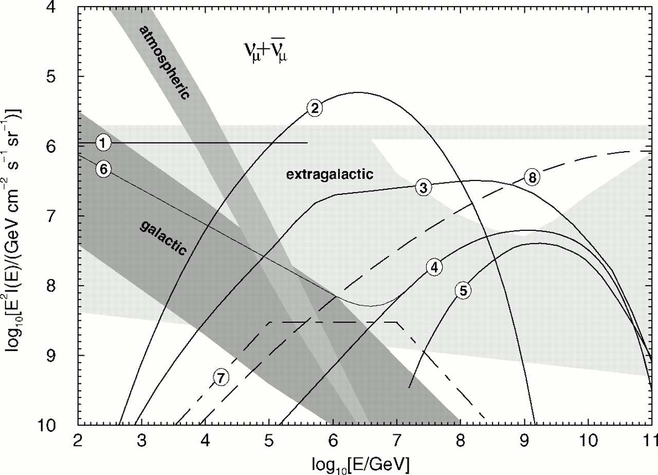
2.7 Expected ?uxes of ? + ?? intensities for emission from various di?use
sources taken from [21]. Fluxes 1-2 are predicted using the core
model of emission from AGNs [22, 23], while ?uxes 3-6 use the
AGN jet (blazar) model [24, 25, 26, 27]. Flux 7 is a prediction of
neutrinos from GRBs [28], while ?ux 8 is a neutrino prediction from
topological defects [18, 19]. . . . . . . . . . . . . . . . . . . . . . 20
3.1 Charged-current neutrino cross sections as a function of energy [33].
The solid line is based on the CTEQ3 parton distributions. The
dashed and dotted lines are from older measurements. . . . . . . 24
3.2 Di?erential cross section for neutrino-nucleon scattering for neu-
trino energies between 10
4
GeV and 10
12
GeV from [33]. . . . . . 25
3.3 Energy dependence of the average in-elasticity of neutrino-nucleon
interactionsfrom[33]. . . . . . . . . . . . . . . . . . . . . . . . . 26
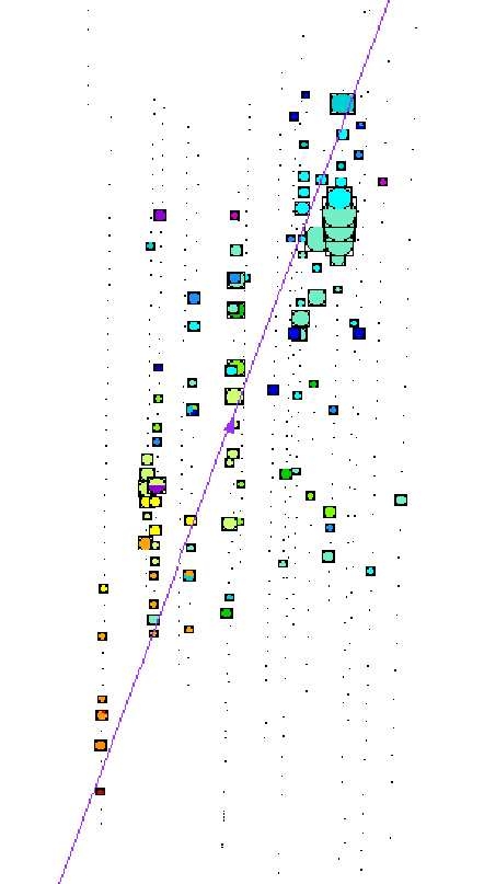
3.4 A muon event in the AMANDA detector. As the muon passes
through the detector, light is emitted at a constant rate. . . . . . 27
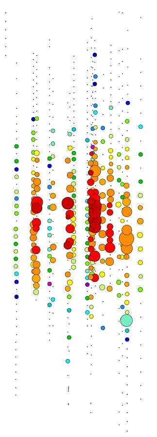
3.5 An electron event in the AMANDA detector. The electron quickly
dissipates its energy in an electromagnetic cascade, generating a
roughly spherical Cherenkov light distribution. . . . . . . . . . . 28
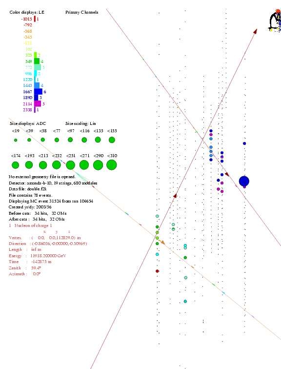
3.6 A tau event in the future IceCube detector. The two cascades of
light are produced by the initial neutrino-nucleon interaction and
subsequent decay of the tau particle. . . . . . . . . . . . . . . . . 30
xiii
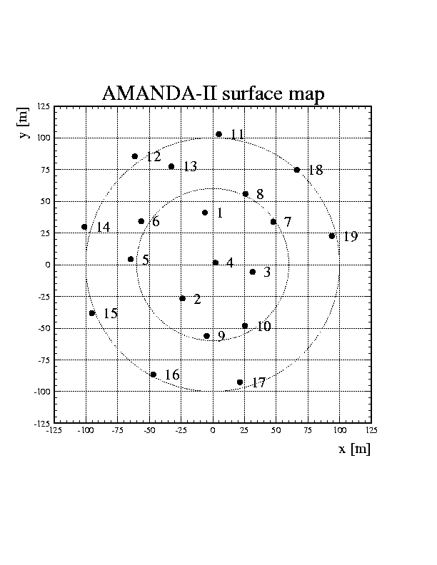
4.1 Top view of the AMANDA-II detector. The radius of the detector
is approximately 100 meters. . . . . . . . . . . . . . . . . . . . . 35
4.2 Schematic of the geometry of AMANDA-II. AMANDA-A and AMANDA-
B10 are shown in expanded view in the center. An optical module
is blown up on the right. The Ei?el Tower is shown to illustrate
thescale. . . . . . . . . . . . . . . . . . . . . . . . . . . . . . . . 36
4.3 Absorption coe?cients as a function of depth at various wave-
lengths[38]. . . . . . . . . . . . . . . . . . . . . . . . . . . . . . 39
4.4 Scattering coe?cients as a function of depth at various wavelengths
[38]. .................................. 40
4.5 Scattering coe?cient as a function of depth, indicating the presence
of dust layers. On the left side of the plot the depth of the OMs in
relation to the dust layers are shown [39]. . . . . . . . . . . . . . 41
5.1 The prior function used is ?at over the up-going hemisphere and
dependent on zenith angle in the down-going hemisphere [36]. . . 46
6.1 The optical modules excluded from the 2000 analysis and their
status. . . . . . . . . . . . . . . . . . . . . . . . . . . . . . . . . 53
6.2 A demonstration of cross talk. The data points that cluster to the
bottom-left of the solid curve are from cross talk. Taken from [48]. 58
6.3 Example of a coincident muon event in the AMANDA-II detector. 60
6.4 Events to the left of the line are primarily due to mis-reconstructed
cosmic ray muons and coincident muons. . . . . . . . . . . . . . 62
xiv
7.1 The energy and zenith angle distributions of atmospheric neutrinos
simulatedfor197days. . . . . . . . . . . . . . . . . . . . . . . . 66
7.2 The zenith angle distribution plotted for events passing level 4 cri-
teria. . . . . . . . . . . . . . . . . . . . . . . . . . . . . . . . . . 67
7.3 The zenith angle distribution plotted for levels 5.1 - 5.4 As quality
parameters are tightened, data and Monte Carlo simulations come
into agreement. The solid line represents data, the dashed line
represents atmospheric Monte Carlo simulations, and the dotted
line represents the E
? 2
Monte Carlo simulations. . . . . . . . . . 68
7.4 The zenith angle distribution plotted for levels 5.5 - 5.8 As quality
parameters are tightened, data and Monte Carlo simulations come
into agreement. The solid line represents data, the dashed line
represents atmospheric Monte Carlo simulations, and the dotted
line represents the E
? 2
Monte Carlo simulations. . . . . . . . . . 69
7.5 The likelihood of the events being up-going. Events to the right-
hand side of the plot are most likely to be from up-going neutrinos.
An excess of data events at lower values than the Monte Carlo simu-
lations indicates that these events are likely to have been produced
by down-going mis-reconstructed muons from cosmic rays rather
than up-going neutrinos. Events to the left of the vertical solid line
areremoved. . . . . . . . . . . . . . . . . . . . . . . . . . . . . . 72
xv
7.6 The distance covered by the muon passing through the detector.
Many mis-reconstructed tracks have lengths less than 155 meters.
Events to the left of the solid vertical line are removed. . . . . . 73
7.7 The distribution of the smoothness of the events in the detector.
High quality tracks have smoothness values near 0. Events between
the two solid vertical lines are kept. . . . . . . . . . . . . . . . . 74
7.8 The number of hits in the detector with time residuals between -15
and 75 ns. A track with high quality would have many \direct"
hits. Events to the left of the solid vertical line are removed. . . 75
7.9 This ?gure demonstrates the disagreement between data and Monte
Carlo simulations for events that have more than 50 optical modules
?red. ................................. 76
7.10 This ?gure shows the disagreement in the smoothness distribution
for events that had more than 50 optical modules ?red. . . . . . 77
7.11 The direct length versus the negative log likelihood ratio of the
the events being track-like to shower-like plotted for events with
at least 50 optical modules ?red and positive smoothness. Events
above and to the left of the solid line are removed. . . . . . . . . 78
7.12 An event removed by the 2D cut on the length of the event versus
the track-to-shower likelihood ratio applied to events with more
than 50 optical modules ?red which had a positive value of the
smoothnessparameter. . . . . . . . . . . . . . . . . . . . . . . . 79
xvi
7.13 The track-to-shower likelihood ratio versus the center of gravity
of the event. Events near the top and bottom of the detector,
where optical modules are more sparsely placed, are required to
demonstrate higher quality than events with center of gravities near
the middle of the detector. Events below and to the left of the
diagonal solid line and the events to the right of the vertical solid
lineareremoved. . . . . . . . . . . . . . . . . . . . . . . . . . . . 81
7.14 The ratio of number of events observed to the number predicted
by Monte Carlo simulations of atmospheric neutrinos. The line ?t
at high event qualities shows the normalization factor used in this
analysis. . . . . . . . . . . . . . . . . . . . . . . . . . . . . . . . 82
7.15 Neutrino energy for the three ?ux predictions used in this analysis.
Below 31 TeV the Lipari and Honda ?uxes agree to within 2.3%
while the Bartol ?ux predicts 23.9 % more neutrinos than the Lipari
?ux. .................................. 85
7.16 The number of optical modules ?red for each event for energies less
than 31 TeV plotted for the three models tested, Lipari, Bartol and
Honda. The number of events for each model has been normalized
totheLiparimodel. . . . . . . . . . . . . . . . . . . . . . . . . . 86
7.17 The number of optical models ?red during each event plotted for
data and the three models tested. The models have been normal-
ized to the number of data events. . . . . . . . . . . . . . . . . . 87
xvii
8.1 As selection criteria are tightened, the number of coincident muon
events for a year diminishes. In the region where the number of op-
tical modules ?red in events is between 50 and 125, an exponential
function can be ?t to levels 3 and 4. Extrapolating this function to
level 5.1 still shows agreement. Extrapolating to level 5.5 shows an
expectation of less than a hundredth of an event each year in the
signalregion(nch>80). . . . . . . . . . . . . . . . . . . . . . . 91
8.2 The muon energy at the center of the detector for atmospheric
neutrinos (background) and E
? 2
neutrinos (signal) before and after
thenchannelcut. . . . . . . . . . . . . . . . . . . . . . . . . . . 93
8.3 The above plots demonstrate a relationship between the number of
OMs ?red during an event and the reconstructed muon energy at
the center of the detector. . . . . . . . . . . . . . . . . . . . . . . 94
8.4 The number of optical modules ?red during events. The dashed
line represents the background atmospheric neutrino Monte Carlo
and the dotted line represents the signal Monte Carlo. . . . . . . 95
8.5 E?ective area for the cuts used in this analysis. . . . . . . . . . . 97
8.6 Number of channels ?red for the unblinded data sample. . . . . . 101
8.7 Number of channels ?red for the blinded data sample. . . . . . . 102
8.8 Number of channels ?red for the combined data sample. . . . . . 104
xviii
8.9 Comparison of predictions of Charm and the SDSS model of AGN
to the results of this analysis. Also plotted are the AMANDA-B10
results and the AMANDA-II results (this work) for an assumed ?at
E
? 2
spectrum. . . . . . . . . . . . . . . . . . . . . . . . . . . . . 107
9.1 Comparison of IceCube sensitivity after 3 years of operation to the
limitsetwiththiswork. . . . . . . . . . . . . . . . . . . . . . . . 111
1
Chapter 1
Introduction
Mankind has long looked with curiosity at the night sky. Stars and planets pro-
vided not only a source of myths, but also served as valuable navigational tools.
This is likely the reason astronomy is among the oldest of sciences.
Up until the turn of the twentieth century, the only means of observing
the sky was with photons at optical wavelengths. During the twentieth century
photon astronomy expanded to new wavelengths. Modern astronomy looks at the
sky in every band from radio waves to gamma rays. These new ways of seeing the
universe paved the way for discovery. New objects and undreamed phenomena,
such as pulsars, active galaxies, gamma ray bursts, and more were revealed.
A de?ning development for astronomy came in 1912 when Victor Hess dis-
covered cosmic rays. This led to the use of protons and other nuclei as messengers
from space. These new messengers brought with them a whole host of questions
such as concerning their origin and the mechanism that accelerates them. These
questions still puzzle scientists today.
In the past decades a new particle, the neutrino, has lent itself to probing
2
solutions to these questions. As messengers from space, neutrinos have advantages
over photons and cosmic rays since they are not absorbed or de?ected at high
energies. The distance a photon can travel through space falls quickly at PeV
energies as its mean free path length is limited to the Mpc scale [1] while cosmic
rays are de?ected by magnetic ?elds as they travel through space.
The idea of using oceans as sites for large neutrino detector date back to the
1960s [2, 3, 4]. Early attempts to use neutrinos as messengers from space started
with the DUMAND project [5] in 1975. At the time of this thesis, there were
three operational neutrino telescopes (ANTARES, AMANDA-II, and Baikal) and
two neutrino telescopes in the development and prototyping stage, IceCube and
NESTOR.
Much time and care has gone into understanding how to calibrate and an-
alyze the data from the AMANDA experiment. These analyses have been the
topic of many theses and papers. The ?rst result, a glimpse of the atmospheric
neutrino spectrum as seen by the AMANDA detector, was published in a letter to
Nature in 2000 [6]. Since that time, AMANDA has further established itself as a
landmark scienti?c experiment and has published results of analyses on neutrino
point sources [7], di?use ?ux muon and electron neutrinos [8, 9], WIMPs [10], and
supernova [11].
This work has helped to pave the way for the topic of this thesis: the ?rst
search for muon neutrinos from di?use astronomical sources with the AMANDA-II
detector.
3
Chapter 2
High Energy Neutrino Physics and
Astrophysics
2.1 Cosmic Rays
Cosmic rays are perhaps one of the oldest, most puzzling creatures known
to Man. They are known to consist of mostly protons and also heavier atomic
nuclei, yet their origin is not yet fully understood. However, it is clear that nearly
all cosmic rays come from outside the solar system, but from within the galaxy.
The most prevalent theory is that most cosmic rays are accelerated by supernovae
explosions. The case for supernovae explosions is strengthened by the realization
that the ?rst order Fermi acceleration at a strong shock naturally produces a
spectrum of cosmic rays consistent with what is observed.
The energy spectrum of cosmic rays is well described by the power-law
dN
dE
/ E
? ?
(2.1)
where ? is the spectral power index. The value of the spectral index is constant
4
at ? = 2:7 for most energies. However, around 3 PeV, the region known as \the
knee", the slope steepens to a value of ? = 3:0. Observations above 5 EeV, the
region known as \the ankle", indicate a ?atter spectrum. Figure 2.1 shows the
di?erential energy spectrum of cosmic rays.
The same engines that produce the highest energy cosmic rays may also
produce neutrinos. Hence, the search for the origin of the highest energy cosmic
rays and the search for high energy neutrinos are intimately related.
2.1.1 Fermi Acceleration
Fermi acceleration [13, 14] is commonly accepted as the most plausible ex-
planation for the particle acceleration as it can reproduce the observed spectrum
of cosmic rays. The acceleration of particles to non-thermal energies takes place
in supersonic shock waves. These accelerated particles are theorized to be present
in supernovae, jets produced by active galactic nuclei (AGN), and other violent
astronomical objects.
Particles gain energy in Fermi acceleration through the transfer of kinetic
energy from shocked material in repeated \encounters" with the material. First-
order Fermi acceleration describes the interaction of particles with a plane shock
front, while second-order Fermi acceleration describes interactions of particles
with moving clouds of plasma. These scenarios are illustrated in Fig. 2.2 and
Fig 2.3. The main di?erence between the two cases is that in second-order Fermi
acceleration particles can gain or lose energy in a given encounter. However, after
many encounters there is a net gain in second-order Fermi acceleration. The
5
Atmospheric
Neutrinos
Figure 2.1: The cosmic ray spectrum adapted from [12].
6
upstream
downstream
−u
E
E
V = −u + u
2
1
2
1
1
Figure 2.2: First order Fermi acceleration by a plane shock front. Adapted from
[15].
E
E
V
1
2
Figure 2.3: Second order Fermi acceleration by moving, partially ionized gas cloud.
Adapted from [15].
following derivation for ?rst-order Fermi acceleration follows that given in [15].
Consider a relativistic particle with energy E
1
that encounters a plane shock
front at an angle ?
1
as shown in Fig 2.2. In the rest frame of the shock, the particle
has an energy
E
0
1
= ? E
1
(1 ? ?cos?
1
)
(2.2)
where ? and ? ? V=c are the Lorentz factor and velocity of the shock respectively
and the primes denote the quantities measured in the frame moving with the
7
shock. Transforming the energy to the rest frame of the particle gives
E
2
=? E
0
2
(1+?cos?
0
2
):
(2.3)
Since magnetic ?elds in the shock ?eld produce elastic scattering, E
0
2
=E
0
1
. Thus,
the energy change, ?E, for the encounter described by ?
1
and ?
2
is given by
?E
E
1
=
1 ? ?cos?
1
+?cos?
0
2
? ?
2
cos?
1
cos?
0
2
1 ? ?
2
? 1:
(2.4)
Averaging over cos?
1
and cos?
0
2
gives ?E ˘ (4=3)?E
1
= ?E
1
. Thus, a
particle encountering a shock increases its energy in proportion to its original
energy. After n encounters, the particle's energy is given by
E
n
=E
0
(1+?)
n
(2.5)
where E
0
is the energy of the particle before the encounter. The number of
particles to reach an energy E is then given by
n=
log
E
E
0
1+?
:
(2.6)
If the probability of particles escaping the acceleration region is given by
P
esc
, then after n encounters the escape probability is given by
P
n
= (1 ? P
esc
)
n
:
(2.7)
The number of particles accelerated to energies greater than E is then
N(>E) /
1
X
m = n
(1 ? P
esc
)
m
=
(1 ? P
esc
)
n
P
esc
:
(2.8)
8
Substituting n gives
N(>E) /
1
P
esc
?
E
E
0
??
?
(2.9)
where
?=
log
1
1 ? P
esc
log1+?
:
(2.10)
For a di?erential spectrum equation 2.9 takes the form
dN
dE
/
1
?
1
P
esc
?
E
E
0
??
( ? +1)
(2.11)
As shown in [15] for shock fronts the spectral index can be approximated as
? =1+
4
M
2
(2.12)
where M = the Mach number ˛ 1. In this case, the spectral index tends to ? ˘ 1
which corresponds to a di?erential index of (? + 1) ˘ 2 at the source. Neutrinos
that result from Fermi accelerated protons/pions are expected to have this energy
spectrum, E
? 2
, when they reach the earth.
This simpli?ed derivation uses the test particle assumption, meaning the
particles being accelerated did not a?ect the conditions in the acceleration region.
More detailed calculations can result in ? ˇ 2:0 ? 2:4. Taking into account the
known energy-dependent leakage of cosmic rays out of the galaxy modi?es the
spectrum by ?? of 0.3 to 0.6. This leads to a ?nal spectral index for ?rst order
Fermi accelerations is ? ˘ 2:7 for cosmic rays [15].
9
2.2 Neutrinos as a Source of Information
The universe has been explored throughout the electromagnetic spectrum,
from radio waves to high energy gamma rays. However, it has not been until
recently that we have been able to examine the universe with a new particle, the
neutrino.
The advantages of using neutrinos as information carriers is demonstrated
in Fig. 2.4. Foremost, neutrinos are not absorbed at high energies by ambient
matter or photon ?elds like their photon counterparts. Photon absorption happens
at the Mpc scale [1] and is the limiting adversary faced by gamma ray astronomy.
Secondly, unlike cosmic rays, which are de?ected by magnetic ?elds as they travel
through space, neutrinos always point directly back to their source.
Astrophysical sources produce high energy gamma rays primarily by radia-
tive processes from accelerated electrons, such as Compton scattering and syn-
chrotron radiation, as well as the decay of pions:
p+? ? ! p+ˇ
0
u
? ! 2?:
(2.13)
In contrast, neutrinos are produced via hadronic processes. The primary sources
of these neutrinos are through the decay of pions and kaons:
p+X ? ! ˇ
?
+Y
u
? ! ?
?
+?
?
(??
?
)
u
? ! e
?
+ ?
e
(??
e
) + ??
?
(?
?
)
(2.14)
10
Accelerator
Target
Opaque matter
N
S
p
p
p
Detector
Earth
p
ν
ν
μ
μ
γ
ν
Figure 2.4: Neutrinos can travel from greater distances than photons because they
are not absorbed by ambient matter or photon ?elds. Furthermore, neutrinos are
not de?ected by magnetic ?elds and always point directly back to their source,
unlike cosmic rays [16].
11
p+X ? ! K
?
+Y
u
? ! ?
?
+ ?
?
(??
?
)
u
? ! e
?
+ ?
e
(??
e
) + ??
?
(?
?
)
(2.15)
p+X ? ! K
0
L
+Y
u
? ! ˇ
?
+?
?
+?
?
(??
?
)
u
? ! ˇ
?
+e
?
+?
e
(??
e
)
:
(2.16)
Hence, high energy astronomy has the ability to di?erentiate between hadronic
and electronic models of gamma ray emitters such as supernovae remnants, gamma
ray bursts, or active galactic nuclei.
2.3 Expected Sources of Astronomical High Energy
Neutrinos
2.3.1 The Atmosphere
Atmospheric neutrinos are produced in abundance in Earth's upper atmo-
sphere. These neutrinos have energies that span a few MeV up to the highest
energy cosmic rays. They serve as both a background and calibration beam in
the search for extraterrestrial neutrinos.
Cosmic rays constantly bombard Earth's atmosphere, producing extensive
air-showers when they interact with nuclei in the air. At the energies relevant
to the AMANDA detector, cosmic rays consist of protons and helium nuclei with
12
some contributions from heavier nuclei. The spectrum of cosmic rays follows a
power law, E
? 2 : 7
, in the energy range of interest for AMANDA.
Cosmic ray nuclei interact producing new particles, such as pions and kaons.
Neutrinos arise primarily from the decay of these pions and kaons as described by
equations 2.14 - 2.16. These neutrinos are referred to as atmospheric neutrinos
because of their origin. The atmospheric neutrino spectrum follows a power law
of E
? 3 : 7
, which is steeper than that of the cosmic rays they come from as shown
in ?g 2.1. The reason for this is that at high energies, pions tend to interact more
often than they decay.
Another reaction that can create neutrinos in the atmosphere is the decay
of charm particles, primarily D mesons. Charmed particles have a short lifetime.
Consequently, the neutrinos that arise from these decays are referred to as prompt
neutrinos. Prompt neutrinos constitute only a few percent of the neutrino ?ux
at 1 TeV and become a dominant source of neutrinos in the atmosphere only
at higher energies. The precise energy and ?ux of prompt neutrinos is heavily
model-dependent.
Although the angular distribution of cosmic rays is isotropic, the spectrum
of atmospheric neutrinos is dependent on zenith angle. Near the horizon the ?ux
is more prominent. This is because pions, kaons, and muons produced nearly
tangent to Earth have longer ?ight times through the atmosphere. Thus, they
have more of a chance to decay into neutrinos. The e?ect is seen as a symmetric
peak in zenith angle about the horizon in Fig 2.5.
13
Cosine Zenith Angle
10
3
10
4
-1 -0.8 -0.6 -0.4 -0.2 0 0.2 0.4 0.6 0.8 1
Figure 2.5: The atmospheric neutrino spectrum has a symmetric peak about the
horizon.
14
2.3.2 The Galactic Disk
Galactic neutrinos are produced through the hadronic interactions that hap-
pen when cosmic rays di?use though the interstellar medium. Most of the energy
lost in these interactions goes into the production of mesons. These mesons sub-
sequently decay into gamma rays and neutrinos. Since there is no atmosphere in
the galactic disk, most of the mesons produced decay into neutrinos. Hence, the
spectrum of gamma rays and neutrinos resembles that of the cosmic ray spectrum
in the interstellar medium,
dN
dE
= E
? 2 : 7
. The ?ux of galactic neutrinos is small
and they have a steep spectrum. Thus, they only become an issue above 1 PeV
(see Fig. 2.7). Even then, the AMANDA detector's location at the south pole
makes galactic neutrino detection challenging. Thus, they pose no background to
this analysis.
2.3.3 Active Galactic Nuclei (AGN)
One promising source of extragalactic neutrinos is active galactic nuclei
(AGN). AGN are among the most energetic objects in the universe. They emit as
much energy as an entire galaxy, but are extremely compact. Their luminosities
have been observed with ?ares extending over periods of days. The frequency of
the ?aring can vary from hours to years. All wavelengths of radiation from radio
waves to TeV gamma rays are emitted from AGN.
AGN are believed to be powered by accreting super-massive black holes
lurking in the centers of galaxies. There are two generic models for neutrino
production in AGN: core models and jet models. The main di?erence in these
15
models is where the neutrinos are produced.
In core models, the neutrinos are believed to be produced in Fermi shocks
of protons inside the accretion disk. The shocked protons interact with protons
or photons in and around the disk producing neutrinos though pion decay as
demonstrated in equation 2.14.
In AGN jet models some of the in-falling matter from the accretion disk is
believed to be re-emitted and accelerated in highly energetic beamed jets that are
aligned with the axis of rotation of the black hole as shown in Fig 2.6.
The particles in the relativistic jet are assumed to be accelerated by Fermi
shocks in clumps or sheets of matter traveling along the jet with Lorentz factors
of 10-100.
Gamma rays can be produced from electron acceleration by synchrotron
radiation or Compton scattering. In the case of proton acceleration, the thermal
ultraviolet photons or synchrotron photons provide the dominant target for pion
production. These pions subsequently decay to gamma rays and neutrinos via
equation 2.14. Di?erent neutrino spectra are expected from electrons and photons
and are the subject of debate. An observation of high energy neutrinos from these
sources would help resolve the issue of particle acceleration.
2.3.4 Gamma Ray Bursts (GRB)
Gamma Ray Bursts (GRBs) are the most luminous cataclysmic phenomena
in the universe. They can be characterized by their ?ares, which last from a
few milliseconds to a few seconds and have short rise times on the order of a
16
Jet
black
hole
accretion disk
wind
γ-ray
~10
–2
pc
γ
~– 10
Figure 2.6: Possible production mechanism for AGN. Electrons and possibly pro-
tons, which are accelerated in sheets or blobs along the jet, interact with photons
that are radiated by the accretion disk or produced in the magnetic ?eld of the
jet. Taken from [17].
17
millisecond followed by an exponential decay. GRBs are randomly distributed
across the sky.
Although the powering process behind a GRB is still unknown, the short
rise time indicates that they originate from compact objects with diameter of tens
of kilometers. Possible sources of such objects are hyper-novae which result from
the fusion of neutron stars or super-massive star collapse.
The bursts are believed to be produced by the dissipation of the kinetic en-
ergy of a relativistically expanding ?reball. Gamma rays could be produced by the
decay of neutral pions or emission of synchrotron radiation (possibly followed by
inverse Compton scattering) by relativistic electrons accelerated in the dissipation
shocks.
In this model, the ultra-relativistic expansion of electron-positron plasma
forms a shock wave. Protons may also be accelerated by Fermi acceleration in the
same region the electrons are accelerated. Neutrinos would then be created by
photo-meson production of pions in interactions between the ?reball ?-rays and
accelerated protons.
It is interesting to note that the energy released in a GRB is about the same
needed to produce the highest energy cosmic rays, whose origin are still unknown.
2.3.5 Exotic Phenomena
The highest energy cosmic rays observed have energies above 100 EeV and
are di?cult to explain using conventional Fermi acceleration models of charged
particles. Some models [18, 19] suggest that these ultra-high energy cosmic rays
18
are produced by the decay of super-massive \X" particles released from topologi-
cal defects, such as cosmic strings and monopoles, created in cosmological phase
transitions. \X" particles can be particles such as gauge or Higgs bosons or super-
heavy fermions. These particles typically decay into a lepton and a quark. The
quark is then theorized to hadronize into nucleons and pions. The pions can then
decay into photons, electrons, and neutrinos.
2.4 Di?use Source
The most obvious way to search for the neutrino sources described above
is to identify excesses of neutrinos coming from particular sources in the sky.
However, individual sources of high energy neutrinos may not be bright enough to
be resolved by the AMANDA-II telescope. Fortunately, there are a large number of
sources. Thus, the sources produce an isotropic background of neutrinos with high
energies. A large neutrino detector, such as AMANDA-II is sensitive to di?use
?uxes of neutrinos from unresolved sources. A measurement of this background
could be the ?rst evidence of neutrinos from hidden sources.
Searching for neutrinos from di?use sources, which is the topic of this work,
is much more di?cult than looking for a particular point source in the sky as
there is no directional information. However, high energy neutrinos predicted to
come from di?use sources have a much shallower energy spectrum, (E
? 2
), than
the atmospheric neutrino background, (E
? 3 : 7
).
Theoretical bounds can be made on the di?use ?ux of neutrinos from knowl-
19
edge of the di?use ?ux of gamma rays and cosmic rays. In the case of proton
acceleration, gamma rays and neutrinos are produced in parallel. Despite the fact
that neutrinos escape the source with no further interactions while the gamma
rays cascade to lower energies in the source or scatter with the cosmic infrared
background, the integral energy of these particles is the same within a factor of two
[21]. The EGRET experiment[20] aboard the Compton Gamma Ray Observatory
measured the isotropic di?use gamma ray background intensity as
?(E > 30MeV) = (1:37 ? 0:06) ? 10
? 6
E
? 2 : 1 ? 0 : 03
cm
? 2
s
? 1
sr
? 1
GeV: (2.17)
Taking into account the factor of two mentioned above, the upper theoretical
bound of the neutrino ?ux is on the order of 10
? 6
cm
? 2
s
? 1
sr
? 1
GeV. This limit
can be seen in ?gure 2.7 as the straight upper boundary of the extragalactic region.
A similar argument can be made for sources where both gamma-ray and
cosmic-ray nucleons escape. For an optically thick source, both protons and neu-
trons are trapped in the source and the gamma ray limit applies. However, for
optically thin sources, it is possible for the neutrons to escape the source without
energy loss and inversely ?-decay into cosmic protons outside the source. These
neutrons then travel una?ected by magnetic ?elds in the Universe. The neutrino
upper bound for these sources is represented by the curved upper boundary of the
extragalactic region in ?gure 2.7.
20
Figure 2.7: Expected ?uxes of ? + ?? intensities for emission from various di?use
sources taken from [21]. Fluxes 1-2 are predicted using the core model of emission
from AGNs [22, 23], while ?uxes 3-6 use the AGN jet (blazar) model [24, 25, 26,
27]. Flux 7 is a prediction of neutrinos from GRBs [28], while ?ux 8 is a neutrino
prediction from topological defects [18, 19].
21
2.5 Neutrino Oscillations
Evidence from GeV scale atmospheric and MeV solar neutrino experiments,
Super-Kamiokande [29] and Sudbury Neutrino Observatory (SNO) [30] strongly
suggest that neutrinos oscillate from one ?avor to another. The LSND accelerator
experiment has also reported observing large neutrino oscillations [31]. This result
is controversial and experiments are under way to con?rm or refute it. In order
to accommodate all three experiments a fourth neutrino, the sterile neutrino (?
s
),
which does not interact has been postulated. The following discussion will consider
the simpli?ed case of two-?avor oscillations.
In order for neutrinos to oscillate from one ?avor to another, neutrinos must
be massive, and the eigenstates for weak interactions must be di?erent than those
for free neutrinos. The probability of a neutrino of ?avor ` and energy E
`
that
travels a distance L in vacuum to oscillate to a neutrino of ?avor `
0
is given by
P
?
`
?
`
0
= sin
2
2?sin
2
ˇ
L
L
osc
(2.18)
where sin
2
2? is the mixing angle between the two neutrinos and L
osc
= 4ˇE
`
=?m
2
is the oscillation length in vacuum.
At their source, neutrinos are produced in the ratio ?
e
: ?
?
: ?
˝
˘ 1 : 2 : 0.
Due to oscillations as they travel through space, the ratio observed at Earth is
1 : 1 : 1 [32]. Thus, muon neutrino ?uxes predicted at their source would on Earth
be observed as one-half the predicted ?ux at the source. This should be kept in
mind when interpreting analysis results as many di?use spectrum ?ux theories do
not take this into account.
22
Chapter 3
Detection of Neutrinos
3.1 Neutrino-Nucleon Interactions
It is well known that neutrinos can not be directly detected. However, a
neutrino or anti-neutrino traveling through matter has some small probability of
interacting through charged-current scattering
?
l
+N ! l
?
+X
(3.1)
??
l
+N ! l
+
+X
(3.2)
where l is the lepton ?avor, N is the target nucleon, and X is a combination of
?nal state hadrons. At high energies, the lepton carries approximately half the
energy of the neutrino. From the kinematics of this reaction, the neutrino and
the lepton will be collinear to a mean deviation of
p
h ?
??
2
iˇ
q
m
p
=E?
(3.3)
which is about 1.75 degrees for a 1 TeV neutrino. The other half of the energy is
released in the hadronic cascade, X, producing a bright, relativity localized ?ash
23
of light.
The cross section for the charged-current neutrino-nucleon interaction in the
rest frame of the nucleon (assuming a relativistic outgoing lepton) is [33]
d
2
˙
dxdy
=
2G
2
F
M
N
E
?
ˇ
?
M
2
W
Q
2
+ M
2
W
?
[xq(x; Q
2
) + xq?(x; Q
2
)(1 ? y
2
)];
(3.4)
where ? Q
2
is the invariant momentum transfer from the neutrino to the outgoing
muon, q and q? are the parton distribution functions of the nucleon, G
F
is the Fermi
constant for weak interactions and M
N
and M
W
are the masses of the nucleon
and W boson. The Bjorken scaling variables, x and y, are given by
x=
Q
2
2M
N
(E
?
l
? E
l
)
(3.5)
and
y =1 ?
E
l
E
?
l
;
(3.6)
where x is the fraction of the nucleon's four-momentum carried by the interacting
quark and y is the fraction of the neutrino's energy deposited in the interaction. At
low energies, the neutrino cross section is four times greater than that of the anti-
neutrino and the cross section is dominated by interactions with valence quarks.
However, at high energies their cross sections become equal as they predominantly
interact with sea quarks in the nucleon, shown in Fig 3.1.
At low energies, ? Q
2
˝ M
W
, and the term in parentheses in equation 3.4
can be neglected. In this region, the neutrino-nucleon cross section rises linearly
with the neutrino energy. However, when Q
2
becomes comparable to M
W
, the
cross section grows more slowly, as seen in Figs. 3.3 and 3.2. This transition occurs
24
Figure 3.1: Charged-current neutrino cross sections as a function of energy [33].
The solid line is based on the CTEQ3 parton distributions. The dashed and
dotted lines are from older measurements.
25
Figure 3.2: Di?erential cross section for neutrino-nucleon scattering for neutrino
energies between 10
4
GeV and 10
12
GeV from [33].
at approximately 3.6 TeV. In this same region the average value of y begins to
fall which leads to an increase in the momentum transfer to the muon and, hence,
a longer muon range. The longer muon range helps o?set the slower growth in
neutrino cross section.
3.2 Lepton Signatures
After a neutrino interacts with a nucleon it produces one of three di?erent
leptons. Each of these leptons leaves a distinct signature in neutrino detectors.
Below the critical energy of about 600 GeV, secondary muons from muon neutrinos
deposit their energy continuously at a rate of ˘ 0:2 GeV per meter as they travel in
a nearly straight line through the detector. The resulting experimental signature
is a long linear deposition of light due to Cherenkov radiation, described in section
26
Figure 3.3: Energy dependence of the average in-elasticity of neutrino-nucleon
interactions from [33].
3.3.1, that leaves a track with length of hundreds of meters, kilometers, or even
tens of kilometers, depending on the initial energy of the muon. A typical muon
signature in the AMANDA detector is shown in Fig. 3.4.
The signature for an event produced by interactions from an electron neu-
trino is a bright, spherical deposition of Cherenkov light generated by an elec-
tromagnetic cascade, and is shown in Fig. 3.5. Unlike muons, which have a
long range, electrons quickly dissipate their energy by radiative processes such
as bremsstrahlung and pair production. The electromagnetic cascade reaches its
maximum after a few meters, a small distance compared to the spacing of the op-
tical modules. Thus, an electron-neutrino event in the AMANDA detector looks
like a point source of light.
The most striking lepton signature, not seen in AMANDA due to the detec-
tor's small size, is that of the tau neutrino. When a tau neutrino interacts with a
nucleon, it produces a tau particle and a hadronic cascade at its interaction point.
Subsequently, the tau particle will travel some distance and decay. This decay
27
Figure 3.4: A muon event in the AMANDA detector. As the muon passes through
the detector, light is emitted at a constant rate.
28
29
will produce a second hadronic cascade. This cascade is very di?cult to resolve
from the ?rst, making it indistinguishable from a cascade produced by an electron,
except at very high energies where the tau may travel hundreds of meters. For
events that are contained within the detector, this \double bang" topology is a
very distinctive signature, as seen in Fig. 3.6.
3.3 Muon Energy Loss
3.3.1 Cherenkov Radiation
A charged particle moving through a transparent medium with refractive
index n > 1 with speed v > c=n will produce Cherenkov radiation. Cherenkov
radiation is emitted at an angle of
cos?
C
=
1
?n
:
(3.7)
For energies relevant to AMANDA, ? ˘ 1. The refractive index of ice is n = 1:34.
Substituting these values into equation 3.7 yields
?
c
=41
?
:
(3.8)
The energy loss due to Cherenkov radiation is ˘ 10
3
MeV=cm, relatively
small compared to the total ionization loss of approximately 2 MeV=cm for mini-
mally ionizing particles [35]. Nonetheless, a muon emits ˘ 200 photons/cm, which
is enough for detection [36].
30
Figure 3.6: A tau event in the future IceCube detector. The two cascades of light
are produced by the initial neutrino-nucleon interaction and subsequent decay of
the tau particle.
31
3.3.2 Stochastic Energy Deposition
Muons can lose energy through several mechanisms: ionization, bremsstrahlung,
pair production, and photo-nuclear processes. Ionization is a quasi-continuous
process and can be treated continuously, while the others are stochastic in nature.
The average rate of stochastic energy loss is nearly proportional to the muon en-
ergy. The total rate of energy loss of a muon traveling through ice per unit length
can be parameterized by
?
dE
?
dx
= a(E
?
)+b(E?) ? E
?
(3.9)
where a is the energy loss due to ionization and b ? E is the energy loss due to
stochastic processes [34].
In ice the value of a is approximately 0:2GeV=m [34] and value of b is
approximately 3:4 ? 10
? 4
m
? 1
. Thus, stochastic events are the main component
of energy loss for muons above 600 GeV.
32
Chapter 4
The AMANDA Detector
AMANDA (the Antarctic Muon and Neutrino Detector Array) is an ice Cherenkov
telescope located beneath the ice at the Amundsen-Scott South Pole Station. The
detector is an array of 677 photomultiplier tubes and was built over the course
of ?ve years. Its primary mission is the detection of neutrinos originating from
astrophysical sources.
4.1 History
The ?rst e?ort to build an under-ice neutrino detector was in the austral
summer of 1993/94. Four strings, each with 20 optical modules, were deployed at
depths between 800 and 1000 meters. This detector became known as AMANDA-
A. Studies of the ice properties at these depths showed the absorption length to be
around 200 meters at the peak absorption of the photomultiplier tubes (PMTs)
of 400 nm. At the same time, the scattering length was on the order of 10-20 cm,
a value too small to allow the reconstruction of muon trajectories. The scattering
length was dominated by tiny air bubbles trapped in the ice. It was thought
33
that these bubbles would be absent at 800 m as a result of the phase transition
that occurs as the increasing pressure transform the air bubbles into air hydrate
crystal. However, due to the low temperatures at the south pole, the di?usion
of air molecules into the ice crystalline structure slows down. Thus, the bubbles
only completely disappear at about 1300 m [37].
Learning from the experiences with the AMANDA-A array, the 19 strings of
AMANDA-II were deployed at greater depths (1500m - 2000 m) in stages during
the austral summers from 1995-2000.
4.2 The Detector
The AMANDA detector consists of a three-dimensional array of optical mod-
ules (OMs). Each OM consists of an 8" Hamamatsu PMT housed in a glass pres-
sure sphere. The OMs are connected to the surface by an electrical cable which
serves two purposes. The cable provides the high voltage necessary to operate the
PMT and transmits signals from the PMTs back to the data acquisition (DAQ)
system electronics at the surface.
As the AMANDA detector grew through years of deployment, the hardware
used to construct the detector matured. The ?rst 4 strings of what is now known
as the AMANDA detector (then called AMANDA-B4) were deployed in the aus-
tral summer of 1995-96. These 86 OMs where connected to the surface by coaxial
cable, which provided protection against electronic crosstalk in the cables. Unfor-
tunately, coaxial cable has limitations. Coaxial cable is quite dispersive, resulting
34
in distortion during the course of transmission to the surface (10 ns PMT pulses
arrive at the surface with a width of more than 400 ns). Coaxial cable is also
quite thick, limiting the number of cables that could be bundled together.
For these reasons the next 6 strings, which were deployed during the austral
summer of 1996-97, used twisted pair cables. These 6 strings brought the total
number of OMs in the array to 302. This new array was named AMANDA-B10.
The twisted pair cables had less dispersion (150 ns - 200 ns) and allowed more
cables per string. However, a great deal of electronic crosstalk was observed in
these strings.
During the austral summer of 1997-98 another 3 strings were deployed bring-
ing the total number of OMs to 428. These strings had both optical ?bers and
traditional twisted pair cables. The optical ?bers were essentially dispersion free
and crosstalk free. However, they were quite fragile and nearly 10% were dam-
aged during the refreeze process. Another change in the deployment of these three
strings was that they were to lie at a depth between 1200 m - 2400 m in order to
study the optical properties above and below the detector.
The last strings to be added to the array were strings 14-19 in the aus-
tral 1999-2000 summer. This marked the completion of the AMANDA-II detec-
tor. All OMs on these strings were connected to the surface via optical ?bers
and traditional twisted pair cables. Some of the modules deployed during this
year contained experimental digital technologies under investigation for future ice-
Cherenkov detectors. String 18 is comprised entirely of digital optical modules
35
Figure 4.1: Top view of the AMANDA-II detector. The radius of the detector is
approximately 100 meters.
(DOMs). These modules contained analog transient waveform digitizers (ATWDs)
which record and digitize the signal in situ and then transmit them to the surface.
This technology results in the full retention of waveform information without the
need for optical ?bers. However, the DAQ electronics are buried with the OMs in
the ice, hence, beyond the possibility of repair or upgrade.
The complete AMANDA-II detector contains 19 strings, 677 OMs and in-
struments 0.015 km
3
of ice. It has a diameter of 200 m and a height of 500 m. The
modules on each string are separated by 10 m - 20 m, depending on the string.
The strings are arranged in three concentric circles and separated by 30 m - 60
m. Figures 4.1 and 4.2 show the layout of the AMANDA detector.
36
120 m
snow layer
?✁?
?✁?✂
✂
optical module (OM)
housing
pressure
Optical
Module
silicon gel
HV divider
light diffuser ball
60 m
AMANDA as of 2000
zoomed in on one
(true scaling)
200 m
Eiffel Tower as comparison
Depth
surface
50 m
1000 m
2350 m
2000 m
1500 m
810 m
1150 m
AMANDA-A (top)
zoomed in on
AMANDA-B10 (bottom)
AMANDA-A
AMANDA-B10
main cable
PMT
Figure 4.2: Schematic of the geometry of AMANDA-II. AMANDA-A and
AMANDA-B10 are shown in expanded view in the center. An optical module
is blown up on the right. The Ei?el Tower is shown to illustrate the scale.
37
The ?rst strings of the IceCube detector are scheduled to be deployed in
the austral summer of 2004-05. The entire IceCube array will contain some 4800
OMs, 80 strings and instrument 1 km
3
of ice. It is scheduled to be completed
in 2009-10. All of the OMs in the IceCube array will use the DOM technology.
IceCube will be deployed between the depths of 1400 m and 2400 m.
4.3 Data Acquisition
The AMANDA detector trigger can come from a variety of sources. In
normal mode, the detector is triggered by the detection of photons by a set number
of OMs in a preset window of time (majority trigger). For the AMANDA-II year
2000 data set, 24 OMs were required to receive at least 1 photo-electron in a
2:1 ?sec time period. The trigger rate was approximately 100 Hz.
The data acquisition (DAQ) system, located on the surface, is responsible
for reading out event information and storing it to disk. Information read and
stored by the DAQ includes the leading edge time (LE) and the width or time-
over-threshold (TOT) in the time window ˘ 22?sec before and ˘ 10?sec after
the trigger time. The DAQ also records the amplitude of pulses arriving from the
OMs. The analog digital converter (ADC) information is recorded during a time
window of ? 2?sec around the trigger time. The event time is obtained from a
Global Positioning System (GPS) unit.
A majority trigger in AMANDA is formed based on hit multiplicity. When
an OM detects a photo-electron it sends a pulse to the surface where it is received
38
by a Swedish Ampli?er (SWAMP) which ampli?es the signal. A copy of the signal
is then sent to discriminators where the signal is converted to a 2 ?sec square pulse.
The discriminator sends its output to the Digital Multiplicity Adders (DMAD)
where multiple signals are summed and compared to a preset threshold. In 2000,
this threshold was set at 24 channels. When the sum crosses the threshold, a stop
signal is sent to all time digital converters (TDCs) and a veto of several ?sec is
sent to the trigger. All channels are then read out and the system reset.
4.4 Ice Properties
Understanding the properties of the ice is crucial for the operation of the
AMANDA-II detector. Thus, the scattering and absorption properties, which
a?ect the timing and number of photons that reach the OMs, must be throughly
understood. Numerous studies using both in-situ light sources and atmospheric
muons have been conducted to determine the ice properties.
The ice is characterized using three parameters: the scattering length ?
b
(or
the scattering coe?cient b = 1=?
b
), the absorption length ?
a
(or the absorption
coe?cient a = 1=?
a
), and the average of the cosine of the scattering angle (˝
s
=
h cos? i . The e?ective scattering length is then de?ned as ?
eff
b
= ?
s
=(1 ? ˝
s
) and
its coe?cient is b
e
= 1=?
eff
b
. The e?ective scattering and absorption coe?cients
are shown in Figs. 4.3 and 4.4 as a function of wavelength.
Dust grains (about 0.04 microns in size) are the biggest contributors to
scattering and absorption in the antarctic ice below 1400 meters. Air bubbles,
39
1200
1400
1600
1800
2000
2200
2400
0.01
1/100
0.02
1/50
0.03
1/33
0.04
1/25
0.05
1/20
0.06
1/16
0.07
1/14
0.08
1/12
0.09
1/11
0.007
1/143
0.008
1/125
0.009
1/111
absorption coefficient
[
m
-1
]
depth
[m]
λ
= 532 nm
λ
= 470 nm
λ
= 337 nm
λ
= 370 nm
Figure 4.3: Absorption coe?cients as a function of depth at various wavelengths
[38].
which were the largest scatterers in the AMANDA-A detector, are squeezed into
air hydrate crystals which have nearly the same index of refraction as ice at
AMANDA-II depths and pose no problems to light detection.
Although the glacial ice in which AMANDA-II is embedded is nearly uni-
form, climatological events in Earth's past, such as ice ages, have left layers of
impurities in the form of dust, soot, etc. These dust layers a?ect the optical
properties of the ice and a?ect photon propagation.
The ?rst measurements of the scattering and absorption coe?cients of these
layers was done using a YAG laser at a frequency of 532 nm. Figure 4.5 shows
the e?ective scattering coe?cient as a function of depth in the detector. The dust
40
800 1000 1200 1400 1600 1800 2000 2200 2400
1
0.1
0.02
1/1
1/10
1/50
scattering coefficient
[
m
-1
]
depth
[m]
A
BC
D
bubbles
dominate
λ
= 532 nm
λ
= 470 nm
λ
= 337 nm
λ
= 370 nm
Figure 4.4: Scattering coe?cients as a function of depth at various wavelengths
[38].
layers are visible as peaks in the scattering coe?cient while the clear layers are
visible as valleys.
41
Figure 4.5: Scattering coe?cient as a function of depth, indicating the presence
of dust layers. On the left side of the plot the depth of the OMs in relation to the
dust layers are shown [39].
42
Chapter 5
Event Reconstruction and Analysis
Tools
Reconstruction algorithms in AMANDA, like the hardware used to build it, have
developed over time. Reconstructions for both muon tracks and cascades are based
on the principle of maximization of a likelihood function. Due to how sparsely
the AMANDA detector is instrumented, only a limited set of parameters can
be constrained for each event. For muons, these parameters are direction (?; ˚),
position(x; y; z), and time (t).
5.1 Direct Walk Reconstruction
The direct walk [40, 41, 42] method of reconstruction is a ?rst guess method
of reconstruction based on pattern recognition of selected hits from photons that
have not scattered much in the ice. First guess methods of reconstruction are very
fast analytic algorithms that are used as initial track guesses for more complicated
algorithms which will be described in the following sections.
43
The direct walk algorithm looks for track elements which are pairs of hits
consistent with a close track such that
?
?
?
?
j r~
1
? r~
2
j
c
? j t
1
? t
2
j
?
?
?
?
<30ns
(5.1)
where r~
i
is the position of the ith hit and t
i
is the time of the ith hit. Associated
hits, those with small time residuals and appropriate distance from the track
element based on time residuals, are selected. Quality criteria such as the number
of associated hits, the spread of associated hits, and the hit density along the
track element are applied. Track elements that pass these criteria are called track
candidates. The ?nal ?rst guess track is then found by searching for clusters in
zenith angle of track candidates and calculating the mean of all track candidates
belonging to the cluster.
5.2 Maximum Likelihood Reconstruction
The maximum likelihood method [42] is a generalization of the ˜
2
method.
In the limit of Gaussian uncertainties the likelihood, L , is related to ˜
2
by
? 2ln L = ˜
2
. These methods attempt to ?nd the track hypothesis that max-
imizes the likelihood by minimizing ? log L with respect to the track parameters.
In general, the likelihood for a given event E
0
, which is a collection of detector
responses R
i
and a hypothesis H
j
, is written as
L (E
0
j H
j
) =
Y
i
L
i
( R
i
j H
j
):
(5.2)
If the hypothesis is true, it then generates the observed pattern of hits. The
hypothesis is then allowed to vary and an optimization routine is used to ?nd
44
the location H
0
of the global extremum of L . The responses f R
i
g recorded by
AMANDA are the time, t
i
, and duration, TOT
i
, of each PMT signal and the peak
amplitude, A
i
, of the largest pulse in each PMT.
In the case of muon reconstruction, one assumes that the Cherenkov radi-
ation is generated by a single in?nitely long muon track. This is a reasonable
assumption for the energies of this analysis which simpli?es and speeds up the
calculation and optimization. For muons, this reduces the function H to six-
dimensions H = H (~x; ?; ˚; t).
5.2.1 Time Likelihood
By applying the assumption of an in?nitely long muon track we arrive at
the simpli?ed likelihood function. The function depends on the arrival time of the
light,
L =
nhits
Y
i =1
p
?
t
i
res
j d
i
; ?
i
:::
?
;
(5.3)
where t
i
res
is the time delay, d
i
is the distance of the OM from the track, and
?
i
is the orientation of the OM relative to the track. The probability density
function of single photons, p (t
i
res
j d
i
; ?), was generated by parameterizing Monte
Carlo simulations of photon propagation in ice [43].
The negative logarithm of the likelihood function, ? log L , is then minimized
using a Simplex [44] algorithm in an iterative technique, which performs multiple
reconstructions of the same event. Each reconstruction starts with a di?erent
initial track hypothesis. The results of all iterations are compared to each other.
45
The lowest value of ? log L is taken as the reconstructed track.
5.2.2 Bayesian Likelihood
Bayes' theorem allows us to fold in information independent of the measure-
ment into the likelihood function. The theorem states
P (A j B)P (B) = P (B j A)P (A):
(5.4)
Identifying A with the hypothesis H and B with the hit pattern E and solving
for P(H j E) gives
P (H j E) =
P (E j H)P (H)
P (E)
:
(5.5)
The quantity P (E j H) is the likelihood that the given set of hits would be gener-
ated by the hypothesis of interest. P (E) is the probability that a given pattern of
hits is observed. This quantity is independent of track parameters and is therefore
constant. P (H) is known as the prior and does not depend in any way on the
measurement. It is the probability of observing the track and can be calculated
prior to the measurement. Thus, P (H j E) is the probability of the hypothesis
after E is taken into account.
Bayesian event reconstruction [45] uses the prior probability function shown
in Fig. 5.1. This function is ?at over the up-going hemisphere and dependent on
zenith angle in the down-going hemisphere. Reconstructing using this technique
requires one to maximize the product of the probability density function and the
prior. Similar to the time likelihood reconstruction, this is done using the Simplex
minimizer and an interactive minimizing technique.
46
Trigger-Level Prior Function
Cos(Zenith)
1
10
10
2
10
3
10
4
10
5
10
6
-1 -0.8 -0.6 -0.4 -0.2 0
0.2 0.4 0.6 0.8
1
Figure 5.1: The prior function used is ?at over the up-going hemisphere and de-
pendent on zenith angle in the down-going hemisphere [36].
47
Near the horizon the e?ect of the Bayesian reconstruction is strongest. Since
AMANDA-II is narrow, events coming in near the horizon have shorter track
lengths, making it di?cult to constrain the ?t tightly. The prior indicates that
tracks from atmospheric muons are more likely than neutrinos. Thus, the recon-
struction properly chooses the down-going ?t as being more likely.
5.3 Quality Parameters
Quality parameters are used for selection criteria during di?erent stages of
the analysis. Below are descriptions of the parameters that will be used for this
analysis.
5.3.1 Likelihood Ratio
As discussed in the previous section, a Bayesian maximum likelihood ?t is
performed on the sample to ?t muon tracks to the observed events. The functional
form used is the negative logarithm of the likelihood. This analysis uses two
likelihood ratios, up-to-down and track-to-cascade. The likelihood ratio for up-
to-down going events is de?ned as
R
u=d
L
= log(
L
up
L
down
)
(5.6)
and the likelihood ratio for track-like to shower-like events is de?ned as
R
t=s
L
= log(
L
track
L
shower
):
(5.7)
L
up
is the likelihood of the track being up-going and hence from a neutrino and
L
down
is the likelihood of the track being down-going and hence from a cosmic
48
ray. L
track
is the likelihood of the event being from a muon and L
shower
is the
likelihood of the event being from a cascade.
The up/down likelihood ratio is the most powerful parameter for separating
cosmic ray background events (down-going) from signal neutrinos (up-going).
5.3.2 Smoothness
\Smoothness" (S
phit
) is a topological parameter that is de?ned by the dis-
tribution of hits along the track. It measures how consistent the observed pattern
of hits is with the hypothesis of constant light emission by a muon.
5.3.3 Number of Direct Hits
A \direct hit" occurs when a photon is delayed little by scattering in the
ice between production and detection. This delay is measured relative to the
predicted arrival time of an unscattered Cherenkov photon emitted from the ap-
propriate point along the track. Di?erent delay windows exist for counting direct
hits. For this analysis a hit is considered direct when it arrives in a window of
[-15:75] nanoseconds. Thus, N
[ ? 15:75]
dir
, is de?ned as the number of direct hits in an
event.
5.3.4 Track Length
The track length is determined by projecting each of the direct hits onto the
reconstructed track and measuring the distance between the ?rst and last hits.
In this analysis, two di?erent track lengths were de?ned. The ?rst uses a stricter
direct hit de?nition than described above. For this track length, the direct hits
49
are required to arrive in the time window [-15:25] nanoseconds
L
[15:25]
dir
(5.8)
and the second uses the de?nition of direct hits from above
L
[15:75]
dir
(5.9)
where direct hits were required to arrive in the [-15:75] nanosecond window.
5.3.5 Zenith Angle
In this analysis, the zenith angle of the best up-going ?t and the zenith angle
of the best down-going ?t are also used in conjunction with the number of direct
hits of the best up-going ?t and the number of hits of the best down-going ?t to
remove coincident muon events from cosmic rays.
5.3.6 Center of Gravity
The center of gravity (
?
cog
!
) of an event is de?ned as the mean position of all
OMs hit by one or more photons in an event. It is represented mathematically as
?
cog
!
=
1
nch
X
nch
i =0
r~
i
(5.10)
where nch is the number of OMs to receive at least one photon and r~
i
is the
distance from the center of the detector to the center of the event.
5.4 The Model Rejection Potential
An upper limit on an expected ?ux can be derived from observation when
an experiment fails to detect an expected ?ux. The method used in this thesis is
50
the model rejection potential [47]. It uses the method developed by Feldman and
Cousins [46] to ?nd the limit. In the Feldman and Cousins method, the upper
limit, ?, is a function of the number of observed events, n
o
, and the number of
predicted background events, n
b
,
? ? ?(n
o
;n
b
):
(5.11)
The ?ux limit is then calculated by the formula
?
CL
= ? ?
?
?
CL
n
s
?
(5.12)
where CL is the desired con?dence level of the calculation, ? is the expected ?ux,
and n
s
is the number of signal events predicted from that ?ux.
Since the actual upper limit cannot be known until looking at the data,
simulations can be used to calculate the expected average upper limit. The average
upper limit is the sum of the expected upper limits, weighted by their Poisson
probability of occurrence. It can be written mathematically as
??
C L
=
X
inf
n
obs =0
?
CL
(n
obs;n
b
)
(n
b
)
n
obs
(n
obs
)!
e
? n
b
:
(5.13)
Using the average upper limit, one can ?nd the optimal selection criteria for
setting the best limit without using the data. When the optimal selection criteria
are applied to the Monte Carlo simulations, they will yield the sensitivity of the
experiment. Over an ensemble of identical experiments, the strongest constraint
on the expected signal ?ux will correspond to the set of cuts that minimizes the
model rejection factor. The model rejection factor is de?ned by
mrf ?
??
C L
n
s
(5.14)
51
where n
s
is the predicted number of signal events from the expected ?ux.
The model rejection factor can then be used to ?nd the expected upper limit
(the sensitivity) de?ned by
??
CL
= ? ?
?
??
C L
n
s
?
:
(5.15)
The actual experiment is not likely to yield exactly ??
CL
. This is because the limit
in that case will be based on the observed number of events, which is subject
to ?uctuations in the background in that particular experiment. The sensitivity,
which is the average ?ux upper limit, would give the average value expected over
repeated runs of a real experiment.
52
Chapter 6
Data and Monte Carlo Simulations
6.1 Live-Time
The total data acquisition time for the year 2000 was 254.2 days. Taking into
account the dead time of the data acquisition system, this corresponds to 211.5
days of detector live time. During that time there were a total of 1,444,252,130
triggers registered. Of those triggers, 90.7% were formed with the majority trigger,
which required at least 24 OMs to have ?red during the event.
File cleaning was performed to remove problematic ?les. A problematic ?le
is one that has at least one of the following symptoms
N
hot
> 5
(6.1)
N
dead
> 50
(6.2)
N
unstable
> 10
(6.3)
where N
hot
is the number of OMs with ADC and/or TDC rates greater than 30
Hz, N
dead
is the number of OMs with ADC and/or TDC rates less than 0.5 Hz,
53
Figure 6.1: The optical modules excluded from the 2000 analysis and their status.
and N
unstable
are the number of OMs with unstable ADC and/or TDC rates. The
?le cleaning removed about four percent of the events and reduced the detector
live time to 197 days for the year.
6.2 OM Selection
An OM is considered bad if the ADC and/or TDC rate is too high, too low
or zero, or if the number of edges from the TDC is too high. Figure 6.1 shows the
OMs excluded in 2000.
In addition to the OMs above, other OMs were excluded on a time-dependent
basis in an attempt to increase the e?ective area of the detector. These OMs
demonstrated transient behavior, meaning at certain times of the year the OM
operated normally and at others the ADC/TDC rates demonstrated the behavior
described above. In order to do this most e?ciently, the year was divided into
54
three periods, with period 1 covering days 44 - 125, period 2 covering days 126 -
244, and period 3 covering days 245 - 315.
6.3 Hit Cleaning
The data recorded by the AMANDA detector are not perfect. Each event
has apparent hits due to various types of noise. The OMs themselves produce
some of this noise; there is dark noise from the PMTs and noise produced by the
decay of the radioactive potassium isotope
40
K in the glass sphere which encases
the PMT. The PMTs are also subject to pre-pulsing and after-pulsing. There is
randomized cross-talk between OMs which can occur in the strings themselves
or the surface electronics. In addition to all this, there is electronic noise in the
DAQ.
Several criteria are used to reduce the number of hits due to noise. The
calibrated amplitude is required to give a reasonable number of photoelectrons,
0:1pe < ADC
calib
< 1000pe. To eliminate random noise at the beginning and
after-pulsing at the end, the event duration window is reduced to ? 2000 ns < LE <
4500ns. Requirements of minimal amplitudes, ADC > 20mV, and time over
thresholds, 124 ns < TOT
elec
< 2000 ns for electrical and 5 ns < TOT
elec
< 2000 ns
for optically read out channels, reduces the electronic noise and electrical cross-
talk. Finally, an isolation cut requiring a hit to be within 100 m and 500 ns of
another hit eliminates hits due to random noise.
55
6.4 Filtering
The AMANDA data used in this thesis were recorded between February 13,
2000 and November 6, 2000. Over 1 billion events in 37,838 ?les took up 1.41 TB
of disk space prior to ?ltering. Each ?le consists of approximately 10 minutes of
data which were recorded by the DAQ electronics. The ?les were grouped into
runs. Each run usually corresponds to one day of data taking. All ?les were then
written to magnetic tape and transported north for ?nal processing and storage.
The data used in this thesis were processed at the DESY Laboratory in
Zeuthen Germany. Doing a complete 16-iteration maximum likelihood reconstruc-
tion as described in section 5.2 is not practical with AMANDA's current resources.
A 16-iteration maximum likelihood reconstruction takes approximately 1 second
per event. Processing all 1.4 billion events would take approximately 4 months
with the current AMANDA resources. As a consequence the AMANDA data is
put through a series of ?ltering levels described below.
6.4.1 Level 1
In lieu of the full maximum likelihood reconstruction, a quick direct walk
reconstruction as described in section 5.1 is performed on all events. This is the
?rst ?t placed on the data. Only events which pass the following cut
?
DW
> 70
(6.4)
are allowed to remain in the data set.
A full 16-iteration maximum likelihood reconstruction is then performed on
56
the remaining events. Another cut is placed on the data set,
?
fullfit
> 70:
(6.5)
The passing rate, after all selection criteria of level 1 are implemented, is 1%.
6.4.2 Level 2
The data set is reduced further at the second level of data ?ltering. The
?rst step of the level 2 ?lter is to place the following cut to the data
?
fullfit
> 80
(6.6)
where fullfit refers to the maximum likelihood reconstruction of level 1. Then six
more reconstructions, including a multi-photon, a Bayesian, and several cascade
reconstructions, are applied to the remaining data set. The passing rate of the
level 2 ?lter is 0.4%
6.5 Background Reduction
After the general ?ltering and cleaning procedures were applied, there were
still non-neutrino backgrounds remaining in the sample. Further cleanings were
performed to remove these backgrounds. These backgrounds can be attributed to
electronic cross talk, coincident muon events from cosmic rays, and mis-reconstructed
cosmic rays. Details of the procedures are described below.
6.5.1 Level 3 - Electronic Cross-Talk and Muons from Cosmic Rays
At level three two cleanings were performed. The ?rst cleaning was used
to remove electronic cross talk that results from capacitive coupling between ca-
57
bles. Secondly, a cut was developed to further remove muons in the data sample
resulting from mis-reconstructed cosmic rays at the horizon.
Electronic cross-talk is known to occur between OMs located on the same
strings in the twisted quad cables used in strings 5 - 10 of the AMANDA detector.
This cross-talk cannot always be removed using basic cleaning algorithms. For
this reason, a special hit cleaning was developed.
The ?rst improvement to be made was to increase the TOT cut for hybrid
OMs. Sixteen OMs have hybrid bases that were used for experimenting with
optical transmission of signal to the surface. For normal data taking purposes,
these channels are read out using the electrical output rather than the optical
output. The electrical signal output for these OMs is much wider than that of
normal OMs. Therefore, the minimum TOT requirement was increased from 120
ns to 200 ns for hybrid OMs. Thus, for standard and hybrid OMs, the minimum
TOT required corresponds to ˘ 0.3 pe.
Cross-talk maps of the detector were made for the 2000 data using timing
calibration data. Using these maps, the unphysical regions of the ADC versus
TOT plots were cut out with the program xt-?lt. Figure 6.2 demonstrates visu-
ally how this was done. The boundary between the physical and unphysical region
in the ADC versus TOT space has been ?t by an exponential function. A shift
of 20 mV in ADC and 20 ns in TOT is added to the ADC versus TOT distribu-
tion boundary to account for any ?uctuations. More details about cross-talk in
AMANDA can be found in [48, 49].
58
Figure 6.2: A demonstration of cross talk. The data points that cluster to the
bottom-left of the solid curve are from cross talk. Taken from [48].
59
After the cross-talk cleaning was applied, two reconstructions were per-
formed on the data. The ?rst was the standard 16-iteration maximum likelihood
reconstruction described in section 5.2. The second was a 16-iteration maximum
likelihood reconstruction with a Bayesian weighted prior as described in section
5.2.2. Events that had a likelihood ratio L
u=d
< 25 (meaning they were more
likely to have been produced by cosmic ray muons) were removed from the data
sample.
The data passing rate after this level was 1:0 ? 10
? 4
%. The events removed
by this level were mostly mis-reconstructed muons from cosmic rays and those
that were triggered by electrical crosstalk.
6.5.2 Level 4 - Coincident Muons
The raw trigger rate of cosmic rays is ˘ 100 Hz. That means every once
in awhile two muons will enter the detector within a time scale of ˘ 5?sec,
close enough that they are treated as one \event" even though they are from two
independent air showers. An example of a coincident muon event can be seen in
Fig. 6.3. A detailed calculation of the rate at which these coincident muon events
trigger the detector was performed in [50]. That rate was determined to be 0.69
per second.
At trigger level, the contribution from coincident muon events is quite low.
Unfortunately, the criteria applied to events consider only a single muon hypoth-
esis. This leads to an enhancement of the contribution from coincident muons at
higher levels of the analysis. Therefore, a cut is applied at level 4 to reduce the
60
Figure 6.3: Example of a coincident muon event in the AMANDA-II detector.
61
coincident muon background contribution. That cut is a two-dimensional cut on
zenith angle and the number of direct hits:
zenith(u) ? zenith(d) < 18:0 ? [ndirc(u) ? ndirc(d)]
(6.7)
where u represents the standard 16-iteration maximum likelihood reconstruction
and d represents the Bayesian reconstruction. This cut is demonstrated in Fig.
8.1.
6.6 Simulations
Generation of events, both neutrino and cosmic ray, occurs in three steps.
First muon and neutrino events are generated. Then they are propagated through
the ice to the detector. Finally, the detector response is simulated.
6.6.1 Muon Generation
Atmospheric muons are simulated using the generator CORSIKA [51]. The
cosmic ray spectrum was assumed to be isotropic with a spectral index of ? = 2:73
and energies between 8 ? 10
2
to 1 ? 10
9
GeVnucleon
? 1
. The interaction model
used was QGSJET .
Simulating air showers requires an enormous amount of computer resources.
The ?ux of cosmic ray primaries is isotropic and muons with energies above 600
GeV are de?ected less than 1 degree. For these reasons, an event generated with
CORSIKA is used multiple times by randomizing the azimuth angle and horizontal
coordinates with respect to the detector. An oversampling factor of 100 was
62
0
50
100
150
-20 -10 0 10 20
0
50
100
150
-20 -10 0 10 20
0
50
100
150
-20 -10 0 10 20
0
50
100
150
-20 -10 0 10 20
Δ
N
dir
- cosmic ray
μ
Δ
zenith angle
Δ
N
dir
- coincident
μ
Δ
zenith angle
Δ
N
dir
- atm
ν
Δ
zenith angle
Δ
N
dir
- E
-2
ν
Δ
zenith angle
Δ
N
dir
- data
Δ
zenith
0
angle
50
100
150
-20 -10 0 10 20
Figure 6.4: Events to the left of the line are primarily due to mis-reconstructed
cosmic ray muons and coincident muons.
63
used for this work. Physics ?uctuations due to this oversampling rate are small
compared to ?uctuations due to the geometry and photon propagation.
Muons from neutrino events with energies between 10 GeV and 10 PeV
are generated using NUSIM [52]. Not only does NUSIM generate neutrinos, it also
propagates the neutrinos through the earth and simulates their interactions with
nucleons. If a neutrino-nucleon interaction takes place in the earth, NUSIM will
also propagate the muon through the rock to the rock-ice boundary using the
MUDEDX code, which is based on tables calculated by Lohmann in [53].
6.6.2 Photon Propagation
Photon propagation in AMANDA is done using the program PTD [43]. The
results of this program, mean amplitudes and arrival time distributions as a func-
tion of relative distance and orientation of the receiver, are stored in large multi-
dimensional archives. These archives are known as the photon tables.
6.6.3 Muon Propagation in Ice
Muons from both neutrinos and cosmic rays are propagated through the
ice and detector using MMC [54]. This program is capable of propagating muons
that have energies from 105:7 MeV to 10
11
GeV. Stochastic and continuous energy
losses are calculated for particles with ?E > 100MeV. If ?E < 100MeV only
continuous energy loss due to ionization is taken into account. Ideally, all energy
losses would be treated stochastically. However, as the energy of the particle in-
creases, the number of separate energy loss calculations increases, which increases
64
the computation time [55]. The calculation of the muon's energy loss as it travels
through ice is valid to within 1%.
6.6.4 Detector Response
The detector response to muons beginning with the PMTs and ending with
the DAQ system is simulated using AMASIM [56, 57]. Rather than generating the
timing and number of photon information for each OM itself, AMASIM gathers this
information from tables generated by PTD.
Simulated parts of DAQ include the OM itself, the cable connecting the OMs
to the surface electronics, the SWAMPs (Swedish ampli?ers), the discriminators,
the TDCs, the peak-sensing ADCs, and the trigger logic. A complete list of
detector details and parameters taken into account by AMASIM is too long to list
here. Even though much care has gone into producing the details of the detector
simulation, more work needs to be done.
Some of the parameters needed for the simulation of the detector include
positions of the optical modules and cable lengths. For simulating the OMs them-
selves, one also needs the noise rate, relative sensitivity, 1 photo-electron level,
and the after-pulse probability of each OM.
65
Chapter 7
Atmospheric Neutrinos
Before embarking on the task of searching for high energy neutrinos from di?use
astronomical sources, it is imperative to have an understanding of the di?use ?ux
of neutrinos produced in Earth's atmosphere. These atmospheric neutrinos are
not only a background to any search for high energy neutrinos, they also provide a
known source which can be used to further understand and calibrate the detector.
Figure 7.1 shows the energy and zenith angle distributions of atmospheric
neutrinos for 197 days, which corresponds to the detector live-time of AMANDA-
II for the year 2000. The energy spectrum of atmospheric neutrinos is steeper
than that of their parent cosmic rays. The reason for this is that at high energies
( ˘ TeV), the pions that decay to produce neutrinos at lower energies start to
interact rather than decay. The zenith angle distribution shows a peak in the
atmospheric neutrinos near the horizon due to the longer ?ight times through the
atmosphere that mesons have near the horizon.
66
Log Neutrino Energy (log GeV)
10
-1
1
10
10
2
10
3
10
4
1 1.5 2 2.5 3 3.5 4 4.5 5 5.5 6
(a) Energy distribution of atmospheric
neutrinos.
Zenith Angle
10
-6
10
-5
10
-4
10
-3
10
-2
10
-1
1
10
10
2
10
3
0 20 40 60 80 100 120 140 160 180
(b) Zenith distribution of atmospheric
neutrinos.
Figure 7.1: The energy and zenith angle distributions of atmospheric neutrinos
simulated for 197 days.
7.1 Level 5 - Event Quality
The basic tools used to determine the purity of any particular data set are
simulations of cosmic ray muons, simulations of neutrinos, and the event viewer.
Ideally, Monte Carlo simulations of down-going muons from cosmic rays and neu-
trinos alone would determine the purity. However, the simulations, although
up-to-date with currently accepted theoretical models, are not accurate enough
to be accepted at face value. One example of this is the atmospheric neutrino
?ux, which is input to the signal Monte Carlo. It has an uncertainty of 25% [58]
at energies above 1 TeV.
The discrepancy between the Monte Carlo simulations and the data can be
seen in Fig. 7.2. Plotted in this ?gure are the data and results from cosmic ray
67
zenith angle
data
cosmic ray
μ
coincident
μ
ATM
ν
MC
E
-2
ν
MC
1
10
10
2
10
3
10
4
10
5
80
100
120
140
160
180
Figure 7.2: The zenith angle distribution plotted for events passing level 4 criteria.
muon, coincident muon, atmospheric neutrino, and E
? 2
neutrino Monte Carlo
simulations. By summing the simulation results in this ?gure, it is clear that the
simulations alone can not account for all of the data events.
For these reasons, the idea of event quality was developed and applied at
level 5 of this analysis. At ?rst the quality cuts are applied loosely and deemed
level 5.1 (level 5 processing, quality level 1). The cuts are then gradually tightened
until level 5.8 (level 5 processing, quality level 8), where there are a handful of the
best neutrino candidates left. This method is independent of the normalization
to the neutrino ?ux discussed in 7.2. Figures 7.3 and 7.4 show that as the quality
parameters are tightened, the rate of change in the Monte Carlo and data begins
to agree. This trend can also be seen in table 7.1.
68
0
20
40
60
80
100
120
80 100 120 140 160 180
0
20
40
60
80
100
80 100 120 140 160 180
0
10
20
30
40
50
60
70
80 100 120 140 160 180
zenith angle
[
degrees
]
- level 5.1
zenith angle
[
degrees
]
- level 5.2
zenith angle
[
degrees
]
- level 5.3
zenith angle
[
degrees
]
- level 5.4
0
10
20
30
40
50
60
80 100 120 140 160 180
Figure 7.3: The zenith angle distribution plotted for levels 5.1 - 5.4 As quality
parameters are tightened, data and Monte Carlo simulations come into agreement.
The solid line represents data, the dashed line represents atmospheric Monte Carlo
simulations, and the dotted line represents the E
? 2
Monte Carlo simulations.
69
0
5
10
15
20
25
30
35
40
80 100 120 140 160 180
0
5
10
15
20
25
30
80 100 120 140 160 180
0
2
4
6
8
10
12
14
16
80 100 120 140 160 180
zenith angle
[
degrees
]
- level 5.5
zenith angle
[
degrees
]
- level 5.6
zenith angle
[
degrees
]
- level 5.7
zenith angle
[
degrees
]
- level 5.8
0
2
4
6
8
10
12
80 100 120 140 160 180
Figure 7.4: The zenith angle distribution plotted for levels 5.5 - 5.8 As quality
parameters are tightened, data and Monte Carlo simulations come into agreement.
The solid line represents data, the dashed line represents atmospheric Monte Carlo
simulations, and the dotted line represents the E
? 2
Monte Carlo simulations.
70
Table 7.1: Passing rates of data and Monte Carlo simulations for various quality
levels. The neutrino Monte Carlo has been normalized as described in 7.2.
Level Data Atm. MC E
? 2
MC Atm ? MC Coinc. ? MC
5.1 1388
819
121
69
68
5.2 1009
726
111
33
38
5.3
755
639
101
13
17
5.4
565
516
88
6.1
9.8
5.5
400
391
66
0
3.1
5.6
287
265
50
0
0.7
5.7
112
113
27
0
0
5.8
70
60
18
0
0
Before discussing the cuts developed at this level, it should be mentioned
that cuts for levels 5.1 - 5.5 were based on 16-iteration maximum likelihood and
Bayesian reconstructions. The level 5.5 - 5.8 cuts were based on more accurate
64-iteration maximum likelihood and Bayesian reconstructions.
There are a total of 6 quality cuts used in this analysis. Four of these cuts
are one-dimensional. They are used to remove mis-reconstructed cosmic rays and
coincident muons. All cuts used are based on the quality parameters described in
section 5.3.
R
u=d
L
= log
L
up
L
down
>35
(7.1)
L
[ ? 15:25]
dir
> 155
(7.2)
j S
phit
j < 0:275
(7.3)
N
[15:75]
dir
> 10
(7.4)
Distributions comparing the data to Monte Carlo simulations of atmospheric
71
neutrinos and E
? 2
of the one-dimensional cuts are shown in Figs. 7.5 - 7.8. In
each of these ?gures, all cuts are applied except the one plotted. A vertical solid
line represents the level of cut selected for the quality parameter in each plot.
These plots have been constructed using the 100 percent data sample at level 5.5.
In each plot, the number of Monte Carlo events have been normalized (see section
7.2) to the number of data events observed.
In addition to the one-dimensional cuts described above, a pair of two-
dimensional cuts are applied to the analysis. The ?rst of these cuts was developed
to remove unsimulated background events that ?red more than 50 optical modules
as they passed through the detector. This e?ect is shown in Fig. 7.9. Examining
these events more closely revealed that they had positive values of the smoothness
parameter as seen in Fig. 7.10. This meant that most of the light in the event
was deposited in the second half of the track. The exact cause of these events is
not fully understood. However, these events tend to be more spherical in nature
(indicating shower-like behavior) and they also have shorter track lengths.
The following cut was developed to remove these events and is applied only
to events that have more than 50 optical modules ?red and positive smoothness.
L
[15:75]
dir
<4:3 ? (log
L
track
L
shower
) ? 65
(7.5)
The diagonal line in Figure 7.11 demonstrates the cut made to remove these events
and ?gure 7.12 shows one of the events removed by this cut.
The ?nal cuts were developed to ensure that events passing through only
the very bottom or very top of the detector (where the optical modules are not
72
likelihood ratio
data
ATM
μ
MC
E
-2
μ
MC
1
10
10
2
10
3
40
60
80
100
120
140
Figure 7.5: The likelihood of the events being up-going. Events to the right-hand
side of the plot are most likely to be from up-going neutrinos. An excess of
data events at lower values than the Monte Carlo simulations indicates that these
events are likely to have been produced by down-going mis-reconstructed muons
from cosmic rays rather than up-going neutrinos. Events to the left of the vertical
solid line are removed.
73
track length
data
ATM
μ
MC
E
-2
μ
MC
0
20
40
60
80
100
120
140
160
180
0
100
200
300
400
500
600
Figure 7.6: The distance covered by the muon passing through the detector. Many
mis-reconstructed tracks have lengths less than 155 meters. Events to the left of
the solid vertical line are removed.
74
smoothness
data
ATM
μ
MC
E
-2
μ
MC
0
25
50
75
100
125
150
175
200
-1 -0.8 -0.6 -0.4 -0.2 0 0.2 0.4 0.6 0.8 1
Figure 7.7: The distribution of the smoothness of the events in the detector. High
quality tracks have smoothness values near 0. Events between the two solid ver-
tical lines are kept.
75
number of direct hits
data
ATM
μ
MC
E
-2
μ
MC
0
20
40
60
80
100
0 5 10 15 20 25 30 35 40 45 50
Figure 7.8: The number of hits in the detector with time residuals between -15
and 75 ns. A track with high quality would have many \direct" hits. Events to
the left of the solid vertical line are removed.
76
nch
data
MC nus atm
MC nus E
-2
1
10
10
2
0 20 40 60 80 100 120 140 160 180 200
Figure 7.9: This ?gure demonstrates the disagreement between data and Monte
Carlo simulations for events that have more than 50 optical modules ?red.
77
smoothness
data
MC nus atm
MC nus E
-2
1
10
-0.3
-0.2
-0.1
0
0.1
0.2
0.3
Figure 7.10: This ?gure shows the disagreement in the smoothness distribution
for events that had more than 50 optical modules ?red.
78
200
300
400
500
600
0 50 100 150 200 250 300 350 400
200
300
400
500
600
0 50 100 150 200 250 300 350 400
Likelihood Ratio
[
shower/track
]
- Data
Track Length
Likelihood Ratio
[
shower/track
]
- ATM
μ
Track Length
Likelihood Ratio
[
shower/track
]
- E
-2
μ
Track Length
200
300
400
500
600
0 50 100 150 200 250 300 350 400
Figure 7.11: The direct length versus the negative log likelihood ratio of the the
events being track-like to shower-like plotted for events with at least 50 optical
modules ?red and positive smoothness. Events above and to the left of the solid
line are removed.
79
Figure 7.12: An event removed by the 2D cut on the length of the event versus
the track-to-shower likelihood ratio applied to events with more than 50 optical
modules ?red which had a positive value of the smoothness parameter.
80
as evenly spaced as the middle of the detector) are from neutrinos and not misre-
constructed comsic rays. These additional cuts were applied to tracks that had a
zenith angle less than 120 degrees.
R
t=s
L
= log
L
track
L
shower
> ? 1:1 ? cogz ? 27:5
(7.6)
cogz < 150:
(7.7)
These cuts are shown as solid lines in Fig 7.13.
7.2 Normalization
As mentioned in section 7.1, the ?ux of atmospheric neutrinos is known only
to 25%. In order to account for this fact the simulated neutrino ?ux is normalized
to the observed ?ux of neutrinos. The ratio of the number of data events to the
number of simulated events is plotted as a function of quality level in Fig 7.14. At
low event qualities (< 4), the data are contaminated by background. At higher
quality levels the ratio stablizes at 0.70. This number agrees with the uncertainty
in the atmospheric neutrino ?ux.
7.3 Other Atmospheric Neutrino Models
The model of atmospheric neutrinos used in this analysis was developed by
Paolo Lipari [59] in 1992. His model uses analytic methods to compute the spectra
of neutrinos and anti-neutrinos produced by cosmic rays in Earth's atmosphere.
In order to investigate the uncertainty introduced by the simulations of
atmospheric neutrinos, two other atmospheric models were investigated for this
81
0
50
100
150
200
250
-250 -200 -150 -100 -50 0 50 100 150 200 250
0
50
100
150
200
250
-250 -200 -150 -100 -50 0 50 100 150 200 250
Center of Gravity
[
m
]
- Data
Likelihood Ratio (s/t)
Center of Gravity
[
m
]
- ATM
μ
Likelihood Ratio (s/t)
Center of Gravity
[
m
]
- E
-2
μ
Likelihood
0
Ratio (s/t)
50
100
150
200
250
-250 -200 -150 -100 -50 0 50 100 150 200 250
Figure 7.13: The track-to-shower likelihood ratio versus the center of gravity of
the event. Events near the top and bottom of the detector, where optical modules
are more sparsely placed, are required to demonstrate higher quality than events
with center of gravities near the middle of the detector. Events below and to the
left of the diagonal solid line and the events to the right of the vertical solid line
are removed.
82
8.417 /
3
P1
0.7005
Event Quality
Ratio data/atm mc
0
0.5
1
1.5
2
2.5
3
0
1
2
3
4
5
6
7
8
9
Figure 7.14: The ratio of number of events observed to the number predicted by
Monte Carlo simulations of atmospheric neutrinos. The line ?t at high event
qualities shows the normalization factor used in this analysis.
83
analysis: one by Honda et al. [60] and the other by Agrawal et al. [61]. These
?uxes are known as the \Honda" ?ux and the \Bartol" ?ux respectively. Both
of these models use Monte Carlo simulations to determine their ?uxes. The dif-
ferences in the models primarily come from the assumed primary spectrum of
cosmic rays and the hadronic interaction model in the atmosphere. In calculating
the Honda ?ux, the authors use a higher primary spectrum normalization than
that used by the authors of the Bartol ?ux.
The hadronic interaction model TARGET [62] used by the authors of the Bartol
?ux is a simple phenomenological representation of pion and kaon production in
interactions of protons, pions, and kaons with light nuclei. The program uses
parameterizations of accelerator data for hadron-nucleus collisions with emphasis
on interaction energies around 20 GeV. The authors of the Honda ?ux used more
sophisticated generators designed for studies at accelerators.
In their original work, the authors of the Honda ?ux calculated ?uxes for
neutrinos up to 31 TeV in energy and the authors of the Bartol ?ux calculated
?uxes for neutrinos with energies up to 10 TeV, while the Lipari ?ux is calculated
up to 316 TeV. Futher work by Gaisser [63] extended the Bartol ?ux up to 1 PeV
making it easier to compare with the Lipari predictions and with the AMANDA
data. Although the Honda ?ux predictions do not reach as high as those of
Lipari and Bartol, one still can make comparisons of trends observed at lower
energies. Figure 7.15 shows the absolute ?ux predictions, meaning the ?uxes are
not normalized. The di?erence in number of neutrinos predicted below 31 TeV
84
in energy between Lipari and Honda is 2.3 % while the di?erence between Lipari
and Gaisser was found to be 23.9%.
To properly compare the di?erent models for this analysis ?rst one must
convert to the energy parameter used for this analysis, the number of optical
modules ?red. Because of the uncertainty in the prediction of primary cosmic
rays that produce atmospheric neutrinos, the observable di?erence in the models
that we are interested in is not the total number of neutrinos predicted, but the
spectrum these models predict. Thus, for comparison purposes the models are
normalized to each other. Finally, a cut must be placed at a neutrino energy of
31 TeV, since the Honda ?ux only predicts energies up to that value.
Figure 7.16 shows the results of this analysis. There is no observable di?er-
ence in the energy parameter of this analysis for the three models tested. The data
is plotted against the three di?erent models in Fig. 7.17. The apparent de?cit in
high values of the number of optical modules ?red parameter can be explained by
the fact that no energy cut was made for this plot since it is not possible to know
the true energy of the neutrino in the data.
85
neutrino energy
Lipari
Bartol
Honda
10
-2
10
-1
1
10
1 1.5 2 2.5 3 3.5 4 4.5 5 5.5 6
Figure 7.15: Neutrino energy for the three ?ux predictions used in this analysis.
Below 31 TeV the Lipari and Honda ?uxes agree to within 2.3 % while the Bartol
?ux predicts 23.9 % more neutrinos than the Lipari ?ux.
86
number of OMs fired
Lipari
Bartol
Honda
10
-2
10
-1
1
10
10
2
0 20 40 60 80 100 120 140 160 180 200
Figure 7.16: The number of optical modules ?red for each event for energies less
than 31 TeV plotted for the three models tested, Lipari, Bartol and Honda. The
number of events for each model has been normalized to the Lipari model.
87
number of OMs fired
data
Lipari
Bartol
Honda
10
-2
10
-1
1
10
10
2
0 20 40 60 80 100 120 140 160 180 200
Figure 7.17: The number of optical models ?red during each event plotted for data
and the three models tested. The models have been normalized to the number of
data events.
88
Chapter 8
Searching for a Di?use Flux of High
Energy Neutrinos
The search for neutrinos from di?use astronomical sources was done using a
blinded analysis technique. This technique required that an unblinded sample
(50% of the year 2000 data in this case) be used for developing cuts and analy-
sis techniques, while the remaining 50%, the blinded sample, be untouched until
after all cuts and techniques were ?xed. The unblinded sample is used for the
?nal analysis and the ?nal result will then be free of any bias introduced by the
scientist.
Before presenting the ?nal results, one last review and check on the back-
grounds to this analysis will be given as a ?rm understanding of the backgrounds
is crucial for analyses that search for small signals. Then the ?nal cut on energy
will be optimized and the sensitivity of the experiment calculated. An e?ective
area will be shown based on the ?nal cut selection and the systematic uncertain-
ties will be discussed. Finally, results will be shown for the assumed E
? 2
neutrino
89
spectrum followed by a discussion of the results and limits on other high energy
neutrino ?ux models.
8.1 Background Rejection
There are three main backgrounds to this analysis. Two of the backgrounds
are muonic in origin - cosmic ray muons and coincident cosmic ray muons. The
third background is the atmospheric neutrino background.
8.1.1 Cosmic Ray Muons
Single muons from cosmic rays are rather easy to remove from the E
? 2
signal
sample. This analysis used the techniques described in chapter 7 to remove single
muons from cosmic rays. At the ?nal cut level there is no contamination expected
from single cosmic ray muons.
8.1.2 Coincident Muons
Coincident muons, which occur when two muons from independent air show-
ers enter the detector at the same time and accidentally trigger the detector, are
a little more tricky to remove. Using the cuts described in chapter 6, at the level
chosen for this analysis (level 5.5), 1.7 events from coincident muons are expected
to remain in the sample according to Monte Carlo simulations of these events.
However, in the energy range of particles considered in this analysis (see section
8.1.3), no coincident muon particles were observed.
The di?culty in concluding that this background would not a?ect the ?nal
90
sample is that it is based on limited statistics. Coincident muon Monte Carlo
simulations have been generated for 83.1 days of live-time using approximately
200,000 CPU hours of computation time.
A procedure to extrapolate to larger statistics was developed. This pro-
cedure is demonstrated in Fig 8.1. As the selection criteria are tightened, the
number of events expected from coincident muons diminishes. In the region of
interest for this analysis, an exponential function with a slope of -0.06 can be ?t
to level 3 and level 4 Monte Carlo simulations of coincident muon events. An
assumption was made that this slope would remain constant as the cuts contin-
ued to be tightened. Extrapolating to level 5.1 still showed agreement with the
simulations. Extrapolating further to level 5.5 gave an expectation of less than a
hundredth of an event each year in the signal region. Thus, for this analysis it is
assumed that the signal region of high energy neutrinos will not be contaminated
by coincident muons.
8.1.3 Background Atmospheric Neutrinos
Atmospheric neutrinos are created during cosmic ray showers in the upper
atmosphere. To the AMANDA detector, these neutrinos seem identical to the
high energy E
? 2
signal neutrinos in every way except their energy spectra.
This analysis uses an energy parameter to separate di?use signal neutrinos
from the di?use atmospheric neutrino background. Figure 8.2 uses Monte Carlo
simulations to show the energy spectrum of the muon as measured at the center
of the detector for signal neutrinos and background atmospheric neutrinos. This
91
nchannel
bkgd. rej. level 3
bkgd. rej. level 4
bkgd. rej. level 5.1
bkgd. rej. level 5.5
10
-2
10
-1
1
10
10
2
10
3
0
50
100
150
200
250
300
Figure 8.1: As selection criteria are tightened, the number of coincident muon
events for a year diminishes. In the region where the number of optical modules
?red in events is between 50 and 125, an exponential function can be ?t to levels
3 and 4. Extrapolating this function to level 5.1 still shows agreement. Extrapo-
lating to level 5.5 shows an expectation of less than a hundredth of an event each
year in the signal region (nch > 80).
92
plot shows that not only do the signal neutrinos have higher energy than the
atmospheric neutrinos, the signal neutrinos have a di?erent spectrum.
A very simple, but e?ective, energy parameter is to count the number of op-
tical modules ?red during an event. This parameter is known as nchannel. Figure
8.3 demonstrates the relationship between muon energy at the center of the de-
tector and nchannel using Monte Carlo simulations of neutrino events. Figure 8.5
demonstrates that nchannel is an e?ective parameter for separating atmospheric
neutrinos for E
? 2
signal neutrino events.
8.2 Sensitivity
After deciding how to separate the atmospheric neutrino background from
the E
? 2
signal neutrinos, the detector sensitivity can be calculated. The method
chosen for this analysis is that of the model rejection potential as described in
section 5.4. Sensitivities and cuts based on the number of optical modules ?red
during an event were calculated. The results of the model rejection potential are
outlined in table 8.1.
Table 8.1: Sensitivities and best number of optical modules ?red cut for various
detector live-times.
Live-time [days] Best # OMs Fired Cut Sensitivity [cm
? 2
s
? 1
sr
? 1
GeV]
98.6
80
3:8 ? 10
? 7
197
87
2:4 ? 10
? 7
400
89
1:5 ? 10
? 7
1000
95
0:9 ? 10
? 7
93
muon energy (log GeV)
ATM MC w/o NCH
ATM MC w/ NCH
E
-2
MC w/o NCH
E
-2
MC w/ NCH
10
-3
10
-2
10
-1
1
10
1
2
3
4
5
6
7
8
9
Figure 8.2: The muon energy at the center of the detector for atmospheric neutri-
nos (background) and E
? 2
neutrinos (signal) before and after the nchannel cut.
94
number of OMs fired
muon energy
[
log GeV
]
1
2
3
4
5
6
7
8
0 50 100 150 200 250 300 350 400
(a) Scatter plot of number of OMs ?red
versus muon energy at the center of the
detector.
number of OMs fired
muon energy
[
log GeV
]
0
1
2
3
4
5
6
7
0 50 100 150 200 250 300 350 400
(b) Pro?le plot of number of OMs ?red
versus muon energy at the center of the
detector.
Figure 8.3: The above plots demonstrate a relationship between the number of
OMs ?red during an event and the reconstructed muon energy at the center of
the detector.
95
number of OMs fired
ATM
υ
MC
E
-2
υ
MC
10
-2
10
-1
1
10
0 20 40 60 80 100 120 140 160 180 200
Figure 8.4: The number of optical modules ?red during events. The dashed line
represents the background atmospheric neutrino Monte Carlo and the dotted line
represents the signal Monte Carlo.
96
8.3 E?ective Area
Based on the selection criteria described in chapter 7 and the number of
optical modules ?red cut described above, it is possible to de?ne an e?ective area
for this analysis. The e?ective area is de?ned as
A
eff
?
˝
N
cuts
N
gen
A
gen
˛
(8.1)
where N
cuts
is the number of events remaining in the sample after selection criteria
are applied, N
gen
is the number of events generated in the sample, and A
gen
is the
generation area of the events. An e?ective area given in this fashion is useful for
comparison of theoretical predictions.
8.4 Systematic Uncertainties
The systematic uncertainties associated with the AMANDA detector are
quite large when compared to other high energy detectors. This is due in part to
the fact that neutrino telescopes such as AMANDA use natural media, i.e. ice, as
a detector medium. The optical properties of the ice used by AMANDA are di?-
cult to measure precisely. The process of deploying the optical modules requires
a melting-refreezing process that may drastically a?ect the properties of the ice.
Once deployed, the OMs are inaccessible. Thus, reasons for strange behavior in
any OM after deployment can only be deduced from signals received by the surface
electronics. The theoretical uncertainties associated with neutrino-nucleon inter-
actions are higher for AMANDA compared to those of accelerator experiments,
due to the higher energy particles the AMANDA detector investigates.
97
log
10
(E
ν
)
[GeV]
Effective
ν
Area
[
cm
2
]
0
2
4
6
8
10
x 10000
1
2
3
4
5
6
7
8
9
Figure 8.5: E?ective area for the cuts used in this analysis.
98
The ?ux of atmospheric neutrinos is a convolution of the primary cosmic
ray spectrum with the yield of the neutrinos produced by hadronic interactions
of the cosmic rays in the atmosphere. Uncertainties in the primary cosmic ray
spectrum and properties of relevant hadronic interactions a?ect the uncertainty of
the atmospheric neutrino ?ux. This e?ect has been studied in [58] and is estimated
to be approximately 30%.
The rate of energy loss in ice is not precisely known. The propagation code
MMC used in the AMANDA-II simulations uses the formulas for cross sections which
are valid within 1% [54, 55]. For the energy range from 20 GeV to 10
11
GeV, the
coe?cients a and b from formula 3.9 have an average deviation from the linear
formula between 3% and 5% [36].
Approximations are made by PTD in the implementation of the measurements
of the optical properties of the ice. This can be seen by comparing analysis results
using the KGM ice model, where direct measurements of the optical properties
were used by PTD , to the results of the MAM ice model, which is an evolution
of the KGM model. However, the MAM model corrects the error introduced by
the approximations made by PTD by adjusting the absorption coe?cient of the
ice. The absorption coe?cient in the MAM ice model was derived from ?ts to the
data.
The optical properties of the ice melted during deployment and then re-
freezed in the week following are di?cult to measure. This quick refreezing pro-
cess introduces many air bubbles in the ice nearest the optical modules. A camera
99
was deployed with one of the strings in the 1997-98 season. It indicated that there
was very strong scattering near the optical modules. However, the issue could not
be entirely settled as there was the possibility that the equipment simply failed.
The lasers used for calibration purposes do not have a good line-of-sight through
the bubbly ice to nearby modules. Thus, there are no direct measurements of the
optical properties of hole ice.
Most of the uncertainties described above are absorbed by the normalization
of the Monte Carlo simulations to the atmospheric neutrino ?ux. Thus, in the
?nal analysis, only the atmospheric neutrino spectrum remains as the systematic
uncertainty.
8.5 Results
As previously mentioned, this analysis was done using a blindness technique.
As previously described, this technique required that 50% of the data be \blinded",
meaning that this sample would not be touched until all cuts were re?ned. The
remaining 50% would be used to develop cuts and the analysis technique. The
?nal result would then be reported using only the blinded 50% sample.
The unblinded sample had a total of 222 neutrino candidates and a live-time
of 98.4 days. Using the model rejection potential method described in 5.4, the
number of optical modules ?red cut was placed at 80. The predicted number
of high energy signal neutrino events was 11.8 and the predicted atmospheric
background was 3.3 above the cut. After applying the cut to the data, 6 events
100
remained in the sample. This yielded a limit of 7:0 ? 10
? 7
cm
? 2
s
? 1
sr
? 1
GeV
without systematic uncertainties. Figure 8.6 shows the Monte Carlo distributions
for atmospheric neutrinos and E
? 2
neutrinos along with the distribution in data
for the number of optical modules ?red parameter.
The blinded sample had a total of 178 neutrino candidates and a live-time
of 98.6 days. The model rejection potential method yielded an optimal cut of the
number of optical modules ?red be greater than 80. Again, the predicted number
of neutrino signal events was 11.8 and predicted number of background events
was 3.3 above the cut. After applying the cut to the data, 4 events remained
in the sample giving a limit of 4:5 ? 10
? 7
cm
? 2
s
? 1
sr
? 1
GeV without systematic
uncertainties. Figure 8.7 shows the Monte Carlo distributions for atmospheric
neutrinos and E
? 2
neutrinos along with the distribution in data for the number
of optical modules ?red parameter.
Although it does not follow a strict blinding procedure, combining the sam-
ples together and running the analysis yields interesting results. The combined
sample has 197 days of live-time and contains 400 neutrino candidates. The
optimal number of optical modules ?red cut is 87 according to the model rejec-
tion potential method. Above this cut, there are 21.0 predicted signal high energy
neutrino events and 4.5 predicted atmospheric background neutrino events. There
were 9 events observed above the cut. This yields (without systematic uncertain-
ties) a two sided con?dence band with boundaries of 0:9 ? 10
? 7
cm
? 2
s
? 1
sr
? 1
GeV
on the bottom side and 4:9 ? 10
? 7
cm
? 2
s
? 1
sr
? 1
GeV on the high side. Figure
101
number of OMs fired
data
ATM
υ
MC
E
-2
υ
MC
10
-2
10
-1
1
10
0 20 40 60 80 100 120 140 160 180 200
Figure 8.6: Number of channels ?red for the unblinded data sample.
102
number of OMs fired
data
ATM
υ
MC
E
-2
υ
MC
10
-2
10
-1
1
10
0 20 40 60 80 100 120 140 160 180 200
Figure 8.7: Number of channels ?red for the blinded data sample.
103
8.8 shows the Monte Carlo distributions of atmospheric neutrinos and E
? 2
neu-
trinos along with the distribution in data for the number of optical modules ?red
parameter.
The Poisson error on the observed rate of atmospheric neutrinos is com-
bined with the theoretical ?ux uncertainty to compute the correlations between
background and e?ciency for use in the probability distribution function used
in the con?dence interval construction. The theoretical ?ux uncertainty is taken
about the best-?t ?ux ?^ and extended to ? 0:25 ? ?. To incorporate these sys-
tematic uncertainties in the e?ciencies into the limit calculations the prescription
of Cousins and Highland [64], as implemented by Conrad et al. [65] with the
uni?ed Feldman-Cousins ordering and improved by a more appropriate choice of
likelihood test [66] was used. Results from the three data samples are shown in
8.2.
Table 8.2: Results for the three di?erent data samples.
Sample
Predicted Predicted No. Obs.
Limit w/o Sys.
Limit w/ Sys.
Background
Signal
Events [cm
? 2
s
? 1
sr
? 1
GeV] [cm
? 2
s
? 1
sr
? 1
GeV]
unblinded
3.25
11.80
6
7 : 0 ? 10
? 7
7 : 2 ? 10
? 7
blinded
3.26
11.82
4
4 : 5 ? 10
? 7
4 : 8 ? 10
? 7
combined
4.47
21.04
9
0 : 5 ? 5 : 1 ? 10
? 7
0 : 4 ? 5 : 4 ? 10
? 7
8.6 Discussion of Results
The six remaining events in unblinded sample were scanned using the AMANDA
event viewer. All six events appeared to be of high quality and consistent with a
high energy muon track. Six events is an upward ?uctuation from the predicted
104
number of OMs fired
data
ATM
υ
MC
E
-2
υ
MC
10
-2
10
-1
1
10
10
2
0 20 40 60 80 100 120 140 160 180 200
Figure 8.8: Number of channels ?red for the combined data sample.
105
3.25 background events that gives an upward ?uctuation in the ?nal limit.
Scanning the four events that remained in the blinded analysis, which is the
?nal result of this thesis, reveals one event that appears to be due to a coincident
muon event, while the remaining three appear to be of good quality and consistent
with a high energy muon track. This leads to the conclusion that either the
extrapolation chosen in 8.1.2 is not valid, or we just happened to have an upward
?uctuation of the background from nearly zero to one. To further test these
hypotheses, more coincident muon background will need to be generated.
A positive outcome of these analyses is the fact that both the blinded and
unblinded samples gave similar results, within statistical ?uctuations. This sug-
gests that the cuts chosen were good in the sense that they did not remove single,
isolated background events, but whole classes of events.
Perhaps the most interesting of the results comes from the of the analysis
that combined the blinded and unblinded data sets together. That analysis ap-
pears to give an excess of data events. At face value, it appears that a signal has
been observed with a chance probablility of 3.7%. However, one must be very
cautious of interpreting this result. Firstly, scanning the remaining nine events
revealed one event that appeared to be caused by a coincident muon event en-
tering the detector. Taking that event out of the equation leaves eight events on
a background of 4.5, which leads to a chance probablity of 8.2%. At the 95%
con?dence level, this results in an upper limit of 5:1 ? 10
? 7
cm
? 2
s
? 1
sr
? 1
GeV.
There are three possible explanations for this result. First, it could be
106
unsimulated background. Scanning the signal candidates revealed that one event
appears to be from coincident muons. Futher studies could rule this out. Secondly,
it could be a ?uctuation in the data. Analysis of more data will reveal whether
this is the case. The ?nal possibility is that a signal has been observed.
In conclusion, although the results do not o?er enough evidence to claim
signal at this time, they do o?er tantalizing hope that AMANDA-II may be close
to a discovery.
8.7 Other Models
Four other models of high energy neutrinos were tested for this thesis. Two
of these models SDSS [67, 68] and SSQC [23] are for core models of neutrino
production in AGN. One model, SSBJ [23], makes a prediction for neutrino pro-
duction in the jets of AGN. The ?nal model, CharmD [69], is an optimistic model
for production of charm neutrinos in the atmosphere. The sensitivities of these
analyses are recorded in table 8.3 and the experimental results are recorded in
table 8.4. Figure 8.9 compares Charm D and SDSS model predictions to the lim-
its found in this analysis. Also shown in ?gure 8.9 is a comparsion of published
AMANDA-B10 results to the results of this analysis.
107
log
10
(E
ν
)
[GeV]
log
10
E
2
Φ
ν
(E)
[
cm
2
s
-1
sr
-1
GeV
]
Atmospheric
neutrinos
SS QC
pred.
SS QC
A-II lim.
Charm D
A-II lim.
Charm D
pred.
MACRO E
-2
ν
μ
Baikal E
-2
ν
e
Frejus
ν
μ
(diff. at E
ν
=2.6 TeV)
AMANDA-B10 E
-2
ν
μ
AMANDA-B10 E
-2
ν
e
-7
-6.8
-6.6
-6.4
-6.2
-6
-5.8
-5.6
-5.4
-5.2
-5
3 3.5 4 4.5 5 5.5 6 6.5 7 7.5 8
AMANDA?II E
?2
ν
μ
Figure 8.9: Comparison of predictions of Charm and the SDSS model of AGN to
the results of this analysis. Also plotted are the AMANDA-B10 results and the
AMANDA-II results (this work) for an assumed ?at E
? 2
spectrum.
108
Table 8.3: Sensitivities for other models of high energy neutrinos. The optimal
nchannel cut, predicted number of background events, and predicted number of
signal events are shown. The average upper limit (??(n
b
)) and average model rejec-
tion factor are shown with and without the inclusion of systematic uncertainties.
Sample nchannel
Predicted
Predicted
? ?( n
b
)
? ?( n
b
)
MRF
MRF
cut
Background
Signal
w/o Sys. w/ Sys. w/o Sys. w/ Sys.
SDSS
112
0.85
7.49
3.15
3.24
0.42
0.43
SSQC
101
1.30
17.0
3.49
3.57
0.21
0.21
SSBJ
80
3.25
9.87
4.51
4.69
0.46
0.47
Charm
50
16.2
4.85
8.19
8.85
1.69
1.82
Table 8.4: Experimental results for other models of high energy neutrinos. The
number observed, the predicted number of background events, and the predicted
number of signal events are shown. The experimental limits (event limit ?
o
?
?(n
o
; n
b
)) are given with and without the inclusion of systematic uncertainties.
Sample Number
Predicted
Predicted
? ( n
o
)
? ( n
o
)
MRF
MRF
Observed Background
Signal
w/o Sys. w/ Sys. w/o Sys. w/ Sys.
SDSS
2
0.85
7.49
5.06
5.28
0.68
0.70
SSQC
2
1.30
17.0
4.61
4.68
0.27
0.28
SSBJ
4
3.25
0.87
5.34
5.66
6.14
6.50
Charm
15
16.2
4.85
6.41
6.82
1.32
1.41
109
Chapter 9
Conclusions
A search for neutrinos from di?use astronomical sources has been performed with
the AMANDA-II neutrino detector using the data taken in year 2000. After
reducing the background of ˘ 10
9
down-going cosmic ray induced muons, 4 events
remain in the sample. Monte Carlo simulations predict 3.25 atmospheric neutrino
(background) events and 11.82 high energy E
? 2
neutrino (signal) events for 98.6
days of live-time of the AMANDA-II detector. This yields a limit, including
systematic uncertainties, at the 90% con?dence level of
?
90%
? 4:8 ? 10
? 7
cm
? 2
s
? 1
sr
? 1
GeV:
(9.1)
This is a considerable improvement over the current published result based on
the 1997 di?use ?ux analysis which included 130 days of AMANDA-B10 detector
live-time and produced a result of ?
90%
? 8:4 ? 10
? 7
cm
? 2
s
? 1
sr
? 1
GeV.
This thesis has also investigated the uncertainty introduced by simulation
of the atmospheric neutrino ?ux by studying three di?erent atmospheric neutrino
models (Lipari, Bartol and Honda). The result of this analysis shows virtually no
110
di?erence in the energy parameter, number of optical modules ?red, used by this
di?use ?ux analysis.
With a further investigation of coincident muons in the detector, this anal-
ysis can be easily extended using the 2001 and 2002 AMANDA-II data.
Looking toward the future, the construction of the IceCube detector is sched-
uled to begin in 2004 and end in 2010. IceCube will be a considerable upgrade
from the AMANDA-II detector as it will instrument 1km
3
of ice and contain
˘ 4000 optical modules on 81 strings. After three years of operation, IceCube
will be sensitive to a di?use ?ux limit of ?
90%
? 4:2 ? 10
? 9
cm
? 2
s
? 1
sr
? 1
GeV [70].
Figure 9.1 compares the limit found in this work with the IceCube sensitivity after
3 years of operation.
111
Test Spectrum
IceCube Sensitivity
3 yrs
AMANDA?II Limit
1/2 yr (this work)
Figure 9.1: Comparison of IceCube sensitivity after 3 years of operation to the
limit set with this work.
112
Bibliography
[1] R. Svensson and A. A. Zdziarski. Astrophys. J. 349, (1990), 415-28.
[2] F. Reines. Ann. Rev. Nucl. Science, 10, (1960), 1.
[3] K. Greisen. Ann. Rev. Nucl. Science, 10, (1960), 63.
[4] M. A. Markov and I. M. Zheleznykh. Nucl. Phys., 27, (1961), 385.
[5] J. Babson et al. (the DUMAND Collaboration). Phys. Rev. D, 42, (1990),
3613-20.
[6] E. Andres et al. (the AMANDA Collaboration). Nature, 410, (2001), 441-
443.
[7] J. Aherns et al. (the AMANDA Collaboration). Astrophys. J., 583, (2003),
1040.
[8] J. Aherns et al. (the AMANDA Collaboration). Phys. Rev. Lett., 90, (2003),
251101.
[9] J. Aherns et al. (the AMANDA Collaboration). Phys. Rev. D, 67,
(2003),012003.
113
[10] J. Aherns et al. (the AMANDA Collaboration). Phys. Rev. D, 66, (2002),
032006.
[11] J. Aherns et al. (the AMANDA Collaboration). Astropart. Phys., 16,
[12] http://astroparticle.uchicago.edu/announc.htm
[13] E. Fermi. Phys. Rev., 75 (1949) 1169-1174.
[14] E. Fermi. Astrophys. J., 119 (1954) 1-6.
[15] T. Gaisser. Cosmic Rays and Particle Physics, Cambridge University Press,
1990.
[16] F. Halzen. Private communication.
[17] F. Halzen. Neutrinos in Physics and Astrophysics (Proc. Theor. Advanded
Staudy Inst. at Boulder), P. Langacker, ed. (World Scienti?c, Singapore,
1998) pp. 524-69.
[18] G. Sigl Towards the Millenium in Astrophys., Problems and Prospects. Int.
School of Cosmic Ray Astrophys. 10th Course, Erice, Italy, June 16-23,
1996, ed. M.M. Shapiro, R. Silberberg, J.P. Wefel, p31. Singapore: World
Sci. (1998)
[19] M. Birkel and S. Sarkar. Extremely High Energy Cosmic Rays from Relic
Particle Decays. hep-ph/9804285, June 1998.
114
[20] P. Sreekumar, et al. (EGRET Collaboration). Ap. J., 494 (1998) 523-534.
[21] J. Learned and K. Mannheim. Annu. Rev. Nucl. Part. Sci 50 (2000) 679-
749.
[22] L. Nellen, K. Mannheim, and P. Biermann. Phys. Rev. D 47 (1993) 5270-
5274.
[23] F. Stecker and M. Salamon. Space Sci. Rev 74:341 (1996).
[24] K. Mannheim, R. Protheroe, and J. Rachen. On the Cosmic Ray Bound
for Models of Extragalactic Neutrino Productrion. astro-ph/9812398, July
2000.
[25] K. Mannheim. Astroparticle Phys. 3 (1995) 295-302.
[26] R. Protheroe and P. Johnson. Astroparticle Phys. 4 (1996) 253-269.
[27] J. Rachen and P. Biermann. Astron. Astrophys. 272 (1993) 161-175.
[28] E. Waxman and J. Bachall. Phys. Rev. Let. 78 (1997) 2292-2295.
[29] S. Fukuda, et al. (Super-Kamiokande Collaboration). Phys. Rev. Let., 85
(2000) 3999-4003.
[30] Q. Ahmad et al. (SNO Collaboration). Phys. Rev. Let., 87 (2001) 071301
[31] C. Athanassopoulos et al. (LSND Collaboration). nucl-ex/9709006,
September 2003.
115
[32] V. Barger, S. Pakvassa, T. Weiler, and K. Whisnant. Phys. Let. B 437
(1998) 107-116.
[33] R. Gandhi, C. Quigg, M. H. reno, and I. Sacevic. Astroparticle Phys. 5
(1996) 81-110.
[34] D. E. Groom et al. European Phys. J., C15 (2000) 1. (The Particle Data
Book.) http://pdg.lbl.gov
[35] C. H. V. Wiebush. The detection of Faint Light in Deep Underwa-
ter Neutrino Telescopes. Ph.D. thesis, Physikalisches Institut, Technishe
Hochschule, Aachen (1995).
[36] T. R. DeYoung. Observation of Atmospheric Muon Neutrinos with
AMANDA. Ph.D. thesis, University of Wisconsin-Madison, (2001).
[37] K. Woschnagg et al. (AMANDA Collaboration). In Proc. 26th Int. Cosmic
Ray Conf., D. Kieda, M. Salamon, and B. Dingus, eds. (August 1999)
HE.4.1.15. http://krusty.physics.utah.edu/ icrc/proceedings.html
[38] http://amanda.berkeley.edu/kurt/ice2000/plots/
[39] P. Desiati, personal communication.
[40] P. Ste?en. Direct-Walk: A Fast Track Search Algorithm Without Hit Clean-
ing, Int. Rep. 20010801
[41] P. Ste?en. Direct-Walk II, Int. Rep. 20020201
116
[42] J. Ahrens et al. (AMANDA Collaboration). Submitted to NIM, (August
2003).
[43] A. Karle. In Proc. Zeuthen Workshop on Simulation and Analysis Methods
for Large Neutrino Telescopes, C. Spiering, ed. (July 1998) pp. 174-185.
[44] W. H. Press, S. A. Teukolsky, W. V. Vetterling, B. P. Flannery, Numerical
Recipies in C - The Art of Scienti?c Computing, 2nd Edition, Cambridge
University Press, 1997.
[45] T. R. DeYoung et al. (AMANDA Collaboration). In Durham 2002: Ad-
vanced Statistical Techniques in Particle Physics, pp. 235-241
[46] G. Feldman and R. Cousins, A Uni?ed Approach to the Classical Statistical
Analysis of Small Signals, physics/9711021 (December 1999).
[47] G. C. Hill and K. Rawlins. Unbiased Cut Selection for Optimal Upper
Limits in Neutrino Detectors: The Model Rejection Potential Technique,
astro-ph/02 09350 (September 2002).
[48] I. J. Taboada. Search for High Energy Neutrino Induced Cascades with the
AMANDA-B10 Detector, Ph. D. thesis, University of Pennsylvania, (2002).
[49] http://www.?s.usb.ve/ itaboada/private/amanda/xtalk/xtalk.html
[50] S. Boser. Separation of Atmospheric Neutrinos with the AMANDA-II De-
tector, Diploma thesis, Technische Universitat Munchen, (2002).
117
[51] D. Heck. CORSIKA: A Monte Carlo Code to Simulate Air Showers, Tech.
Rep. FZKA 6019, Forshungszebtrum Karlsruhe (1998).
[52] G. Hill. Experimental and Theoretical Aspects of High Energy Neutrino
Astrophysics, Ph. D. thesis, University of Adelaide, Adelaide, Australia
(1996).
[53] W. Lohmann, R. Kopp, and R. Voss. Energy Loss of Muons in the Range
1-10000 GeV, Yellow Report 85-03, CERN (1985).
[54] D. Chirkin and W. Rodhe. In Proc. 27th Int. Cosmic Ray Conf. eds. K.H.
Kampert, G. Hainzelmann, and C. Spiering, (2001), pp.1017-1020.
[55] http://amanda.berkeley.edu/ dima/stu?
[56] S. Hundertmark. In Proc. of 1st Workshop Methodical Aspects of Under-
water/Ice Neutrino Telescopes, Zeuthen Germany, (1998) pp. 276-286.
[57] S. Hundertmark. Verticle Ice Properties for AMANDA Simulation,
AMANDA Internal Rep. 20001001, (2000).
[58] T. K. Gaisser. Uncertainty in Flux of Atmospheric Neutrinos: Implications
for Upward Muons in AMANDA B10, AMANDA Internal Rep. 20001201,
(2000).
[59] P. Lipari. Astroparticle Phys., 1, (1993), 195-227.
[60] M. Honda, T. Kajita, K. Kasahara, S. Midorikawa. Phys. Rev. D, 52,
(1995), 4985-5005.
118
[61] V. Agrawal, T. K. Gaiser, P. Lipari, and T. Stanev. Phys. Rev. D, 53,
(1996), 1314-1323.
[62] T. K. Gaisser, R. J. Protheroe, and T. Stanev. In Proc. of the 18th Inter-
national Cosmic Ray Conference, ed. N. Durgaprasad et al. (Tata Institute
of Fundamental Research, Colaba, Bombay), Vol. 5, (1983), pp. 174
[63] T. K. Gaisser. Personal communication.
[64] R. D. Cousins and V. L. Highland. Nucl. Ins. Meth. Phys. Res., A320,
(1992), 331.
[65] J. Conrad, O. Botner, A. Hallgren, and C. Perez de los Heros. Phys. Rev.
D., 67 (2003) 012002.
[66] G. C. Hill, Phys. Rev. D, 67, (2003), 118101.
[67] F. W. Stecker, C. Done, M. H. Salamon, and P. Sommers. Phys. Rev. Lett.,
66, (1991), 2697-2700
[68] F. W. Stecker, C. Done, M. H. Salamon, and P. Sommers. Phys. Rev. Lett.,
69, (1992), 2738.
[69] E. Zas, F. Halzen, and R. A. Vazquez. Astropart. Phys., 1, (1993), 297.
[70] J. Aherns et al. (the IceCube Collaboration). Accepted to Astropart. Phys.,
(September 2003). astro-ph/0305196.
119
Appendix A
Reconstruction Chain
Table A.1: Outline of reconstruction chain.
Level 1
reco 1
direct walk
reco 2
maximum likelihood
16 iterations
cut 1 ?
reco 2
> 70
?
Level 2
cut 2 ?
reco 2
> 80
?
reco 3
multi-photoelectron
16 iterations
reco 4
Bayesian likelihood
16 iterations
reco 5
line ?t
reco 6
dipole moment
reco 7
tensor of inertia
amplitude weight = 1
reco 8
cascade likelihood
Level 3
xt-?lter
reco 9
maximum likelihood
16 iteration
reco 10
Bayesian likelihood
16 iteration
Level 4
cut 4 (?
reco 9
? ?
reco 10
) <
18( ndirc
reco 9
? ndirc
reco 10
)
Level 5
cuts 5-11 quality cuts level 5.5
reco 11
maximum likelihood
64 iterations
reco 12
Bayesian likelihood
64 iterations
120
Appendix B
Quality Levels
Table B.1: List of cuts de?ning each quality level. The two dimensional cuts in
the two rows are de?ned by their slope and intercept.
Quality
L
[ ? 15:25]
dir
?L
u=d
j S
P
hit
j N
[ ? 15:75]
dir
L
[ ? 15:75]
dir
<m ??L
t=s
? b ?L
t=s
>m ? cogz ? b
Level
(m,b)
and cogz < 150 (m,b)
1
100.0
30
0.400
5
(4.3,-25)
(-0.22,-5.5)
2
110.0
31
0.370
6
(4.3,-35)
(-0.44,-11.0)
3
120.0
32
0.350
7
(4.3,-45)
(-0.67,-16.75)
4
130.0
34
0.330
8
(4.3,-55)
(-0.89,-22.5)
5
155.0
35
0.275
10
(4.3,-65)
(-1.1,-27.5)
6
170.0
37
0.250
12
(4.3,-70)
(-1.32,-33.0)
7
200.0
40
0.200
15
(4.3,-75)
(-1.54,-38.5)
8
210.0
42
0.180
17
(4.3,-85)
(-1.77,-44.25)
121
Appendix C
Atmospheric Neutrino Event Candidates
Table C.1: List of atmospheric neutrino events.
Event
Day Zenith Azimuth
Right
Declin.
Gal.
Gal.
No.
Asc.
Long.
Lat.
2142814 160 123.301 320.828 15.2945 33.301 53.0652 57.9794
3185887 182 157.48 313.104 1.99119 67.481 129.394 5.46677
3593604 226 171.038 355.539 20.9636 81.038 114.693 22.1963
423496 269 121.552 118.105 1.29468 31.552 129.453 -30.9872
481414 84 126.515 75.4717
23.666 36.516 107.249 -24.1695
1332216 157 160.908 100.636 12.8708 70.907 122.836 46.2211
1760779 188 162.309 259.04
18.1623
72.308 102.969
28.905
1567697 300 128.435 170.983
4.7038 38.435 164.594 -5.1114
2078330 150 148.356 349.003 13.8531 58.357 108.528 57.0691
938626 151 157.079 41.7212 5.49294 67.079 145.411 17.3849
866
154 168.069 226.651 7.74847 78.069 136.26 29.2533
2412706 159 138.845 176.048 0.654423 48.844 120.869 -13.979
672095 164 143.794 212.819 11.9026 53.795 140.655 61.318
3914785 164 141.591 227.981 0.323957 51.592 117.879 -10.9655
938476 177 129.698 334.05
14.2338
39.697 74.445
68.7569
3432923 179 152.855 165.484 12.7188 62.854 124.554 54.2481
1957663 187 171.513 258.842 18.6472 81.513 113.389 27.2718
4974272 201 132.437 52.7352
20.918 42.436 83.6236 -1.70357
3282703 207 165.333 110.991 6.85558 75.332 139.32 26.1691
2135873 216 163.605 300.849 20.3077 73.605 106.718 20.141
955188 218 132.478 332.528 12.8398 42.479 123.662 74.6478
3336654 218 153.976 45.6379
18.925 63.975 94.2921 23.7548
3790473 218 156.349 197.532 10.8865
66.35 139.717 46.738
continued on next page
122
Table C.1: continued
Event
Day Zenith Azimuth
Right
Declin.
Gal.
Gal.
No.
Asc.
Long.
Lat.
2089774 222 149.334 342.856 15.2368 59.334 95.6363 49.5412
3055268 222 130.835 157.585 7.97706 40.835 179.276 29.521
5392785 62 122.563 90.9242 14.7564 32.563 52.2915 64.7812
4953315 236 158.247 34.3877 21.1709 68.246 104.66 13.6336
1697
236 148.436 62.0133 22.1297 58.437 102.87 2.09094
4683242 241 155.039 33.0419 22.0432 65.039 106.304 7.77119
831360 259 128.149 74.2357 15.0015
38.15 63.3937 60.9445
2200836 264 136.095 31.8114 14.9069 46.096 79.1172 59.2005
28561 272 173.878 345.289 8.47128 83.879 129.347 29.4919
3002342 272 150.309 147.378 11.3483 60.309 141.586 53.4168
4839112 273 143.019 41.6718 3.20105
53.02 143.255 -4.21166
2700849 285 134.222 5.96017 20.1339 44.223 80.0084 6.24693
3520175 67 127.734 50.6807
11.27
37.734 179.007 67.3704
215224 292 154.451 190.286 20.9048 64.452 100.618 12.4372
5331635 69 138.732 290.263 1.73171 48.731 131.777 -13.2376
1896065 302 154.624 355.666 19.2475 64.623 95.5759 21.9064
3277996 307 148.84 76.7077
3.83664
58.84 144.316 3.60131
3948769 69 158.846 144.439 6.65749 68.845 146.188 24.1082
898909 72 144.404 62.0627 0.976479 54.405 123.984 -8.45215
1229568 77 169.206 107.723
23.8249 79.207 119.94
16.6968
2851464 78 125.122 30.2293
11.0935 35.123 186.88
66.0701
2377102 88 174.298 312.258
15.2546 84.297
119.
31.6893
4567259 89 146.837 292.785 0.916248 56.836 123.418 -6.03241
715221 90 128.641 331.188
7.77793
38.64 181.109 26.7859
4717507 99 176.852 18.3145
14.1549 86.852 121.72
30.0911
597394 104 143.799 6.95995 23.6347
53.8 112.128 -7.52582
2495921 106 154.377 304.518 10.6756 64.377 143.098 47.3006
2928444 106 163.767 13.0684 7.71865 73.767 141.188 29.5665
3374821 106 144.659 79.0094 5.00195 54.659 153.998 7.56312
471928 108 141.284 78.1579 11.3117 51.284 152.6
60.1678
488352 114 150.548 234.38
4.59569 60.549 147.315 8.79178
224809 121 136.436 261.797 2.43239 46.437 139.425 -13.3861
5726476 53 156.085 15.6118
21.5908 66.084 104.81
10.3767
4384033 136 120.157 184.128 8.67769 30.157 193.819 35.5975
4819501 137 123.046 144.115 13.1171 33.047 94.2192 83.1897
5929236 137 142.154 180.975 15.1854 52.153 86.3581 53.8816
1329751 138 146.12 319.734 11.4465 56.121 144.783 57.2696
5281309 139 139.485 221.383 10.2231 49.485 165.624 52.439
continued on next page
123
Table C.1: continued
Event
Day Zenith Azimuth
Right
Declin.
Gal.
Gal.
No.
Asc.
Long.
Lat.
698547 139 129.877 134.497 21.3088 39.878 84.6945 -6.69083
441286 140 135.683 91.4076 23.2315 45.683 105.646 -13.8893
5303086 144 170.711 90.5342 18.2611 80.712 112.511 28.1859
1326220 147 156.324 253.651 16.5058 66.324 98.1264 38.6074
1355187 147 169.176 279.881 14.8774 79.175 116.178 36.312
2165291 148 168.978 188.852 0.624797 78.977 122.238 16.1241
2159840 150 155.558 334.368
15.179 65.557 103.103 45.8421
5046057 151 156.956 163.441 14.9526 66.957 105.91
45.795
1259101 152 148.04 239.72
17.6913 58.039 86.4415 31.9002
4121944 154 144.777 43.8361 19.7658 54.777 87.5412
14.57
4724656 56 150.867 134.574 10.1481 60.866 150.438 46.6437
4382518 156 164.71 125.773 14.4205 74.709 114.947 40.9323
4132334 158 128.583 4.93843 7.56419 38.583 180.434 24.3551
1451412 158 161.949 152.949
9.931
71.949 139.031 39.2177
1654509 165 163.482 164.479 19.2804 73.481 104.89 24.1542
2116222 165 145.461 236.572 16.4147 55.46 84.7647 42.5894
3681545 165 126.586 65.6443
10.359
36.586 186.78 57.0264
3910453 170 158.705 48.9174 0.123911 68.705 118.935 6.17543
2842511 171 163.534
244.9
6.68018
73.534 141.166
25.188
4576434 177 144.577 258.661 10.7645 54.577 154.075 54.2833
5194469 178 130.772 281.183 12.4235 40.771 142.754 75.3397
2419051 179 151.518 44.3909 16.3034 61.517 92.9051 41.5974
3521648 179 127.045 271.042 6.07552 37.044 174.953 7.48809
2049092 180 176.657 97.4777 11.1914 86.658 124.564 30.1479
475650 182 169.497 12.0137 10.0743 79.497 131.422 34.7077
1796076 183 121.582 225.448 2.00246 31.581 139.658 -29.0493
4895669 185 129.333 13.9474 6.22779 39.332 173.747 10.141
1021126 188 156.129 58.1021 5.53369 66.128 146.405 17.1366
1580120 188 120.343 203.431
21.376 30.343 78.2904 -13.8983
5955415 188 165.616 20.5008 21.5408 75.616 111.473 17.3874
573627 190 143.264 227.942 18.2724 53.265 81.5809 26.5271
5276912 200 142.607 287.681 6.88337 52.608 163.664 21.4671
2137011 202 173.463 328.557
18.956
83.464 115.61 26.7695
967389 203 146.052 234.65
19.9791 56.053 89.5763 13.5559
2658001 59 160.213 254.579 17.7397 70.214 100.699 31.0613
2491556 213 137.589 198.883 4.36925
47.59 155.381 -1.56085
1283256 60 131.393 121.708 21.6951 41.392 88.9558 -8.63567
3368601 60 132.827 260.446 20.0593 42.826 78.3839 6.19648
continued on next page
124
Table C.1: continued
Event
Day Zenith Azimuth
Right
Declin.
Gal.
Gal.
No.
Asc.
Long.
Lat.
332303 224 146.28
212.38
16.0317
56.281 87.1848 45.4234
4844368 226 144.917 77.1417 21.0874 54.916 94.1441 5.22988
332712 234 142.157 16.8533
6.7287 52.158 163.656 19.9813
3373864 234 164.451 188.451
8.8699 74.451 139.162 34.0048
3533809 239 122.233 1.66995
18.687 32.232 61.3614 16.0666
1331839 62 150.488 13.1948 5.32518 60.488 150.675 13.041
2762494 242 130.105 176.537 3.63934 40.104 154.347 -12.3735
1501705 245 142.478 192.181 21.1552 52.479 92.7413 3.14568
1608536 249 122.409 152.723 0.621733 32.408 119.474 -30.3688
2843674 249 136.579 162.221 5.88369 46.579 165.449 10.1921
389600 250 153.437 279.557 10.4432 63.438 145.631 46.799
3014760 250 139.583 30.6523 15.5662 49.584 79.9625 51.7251
3349658 63 138.652 98.9554 7.29776 48.651 168.945 24.2021
4106905 254 131.003 23.7858
21.395 41.003 86.1963 -6.60053
1505225 255 153.091 155.948 0.227849 63.092 118.674 0.532882
1545291 256 130.297 204.843 21.2403 40.296 84.4509 -5.83414
3300293 259 124.642 135.963 22.4683 34.641 92.1952 -19.5373
486914 262 155.036 183.321 20.7263 65.037 100.386 13.7004
2922333 262 165.608 262.665 2.83529 75.608 130.231 14.4459
730347 263 142.868 128.872 1.61213 52.869 129.831 -9.39499
2845681 263 131.118 320.542 22.7049 41.117 98.2515 -15.4844
2957667 263 157.184 175.965 8.86973 67.184 147.552 36.4295
1172768 264 140.891 210.276 22.2424 50.892 99.342 -4.65065
4140788 265 123.744 209.957 12.4412 33.745 160.515 81.4751
2032341 269 152.954 92.715
10.5472 62.953 145.501 47.6486
3415232 269 120.08 359.039 23.2524
30.08 99.2908 -28.3338
1035338 65 154.838 310.995
8.51513 64.839 150.98
34.8786
2880198 276 146.659 66.9023 16.5711 56.66 85.9205 41.0362
3290529 276 146.046 160.172 12.2568 56.045 133.118 60.3651
2469576 277 149.12 217.346
4.60807
59.12 148.457 7.91186
3638945 277 163.501 115.012 16.8253 73.502 105.671 34.4309
2395528 278 165.341 113.902 10.9153 75.34 132.137 39.6347
2828443 279 135.854 153.399 10.3956 45.854 170.334 55.3592
745094 280 156.428 118.967 3.40547 66.429 137.399 7.95208
3618665 280 166.802 4.0705 0.410794 76.802 121.359 14.0121
2783371 66 132.613 272.037 17.8482 42.612 68.8669 28.6687
122072 282 170.758 18.4628
7.336
80.758 133.319 27.9001
1535236 285 133.78 34.7887 12.8876 43.781 121.788 73.3432
continued on next page
125
Table C.1: continued
Event
Day Zenith Azimuth
Right
Declin.
Gal.
Gal.
No.
Asc.
Long.
Lat.
3407046 285 150.139 255.815 6.69194 60.139 155.404 22.1027
3686412 285 146.604 238.912 9.09088 56.604 160.14 40.6245
5212833 288 158.925 188.753 19.0549 68.925 99.7584 24.1381
1630711 294 122.09 35.9698
13.6043
32.09 62.6181 79.0758
2756856 295 163.899 233.49
5.4356
73.9 138.929 20.3861
1546608 296 122.909 77.7734 10.5021 32.908 193.507 59.0175
1320443 297 164.498 203.14
1.21961 74.499 124.413 11.6898
5032179 300 127.737 189.698 18.8912 37.738 67.649 15.8337
2401616 301 136.381 277.629 1.31719
46.38 127.882 -16.2263
1553304 305 137.521 188.737
13.261 47.521 111.434 69.0629
2783736 71 159.939 225.74
20.8142
69.939 104.794 16.1807
5949917 75 128.221 44.9787
21.0613
38.22 81.501 -5.70026
3569875 79 130.102 202.569
2.01478
40.103 137.07 -20.8545
2308452 82 144.615 164.583 0.842262 54.616
122.8
-8.25552
5509929 85 146.403 253.014 7.42531 56.403 160.794 26.9219
5850961 85 122.263 47.632
22.4788 32.263 90.9006 -21.5874
2863674 91
180.
333.446
16.0122
90.
122.932 27.1283
3994675 50 147.359 211.138 2.45243
57.36 135.587 -3.14128
4436099 50 138.402 74.9444 13.1403 48.402 115.234 68.4716
1782730 96 140.309 229.382 12.4651 50.309 132.337 66.3873
2839606 96 143.223 58.7723
3.82969 53.224 147.786 -0.816065
5736570 97 149.732 151.515 8.88832 59.732 156.604 38.4087
2897298 102 146.631 197.718 19.4076 56.631 87.9974 18.0911
3871583 51 133.214 272.339 23.1064 43.214 103.366 -15.631
1208393 111 137.175 20.748
21.6788 47.176 92.6722 -4.18003
545025 115 143.808 113.705
12.83
53.808 123.47 63.3185
1747483 116 167.387 201.448 12.0469 77.387 126.344 39.4173
4294055 117 152.1
43.968
9.2771
62.099 152.669
40.505
4438509 120 170.291 325.107 15.1039
80.29 116.368 35.053
6014534 121 133.209 32.3442 16.5537 43.208 67.9635 42.8522
1349324 122 158.705 359.934 0.387539 68.705 120.365 5.97387
4929757 123 125.609 60.3763 10.7296 35.608 187.596 61.6041
1654462 125 143.525 336.005 8.77144 53.524 164.621 38.3773
2341138 52 132.901 254.129 16.7311 42.901 67.5518 40.9082
2310094 127 123.167 1.08217 10.2397 33.167 193.071 55.7164
1056477 129 122.112 20.9622 3.03159 32.112 152.692 -23.1147
1864962 53 161.971 158.096 21.4393 71.972 108.448 15.1455
2309938 141 158.697 210.139 22.9407 68.698 112.766 8.12682
continued on next page
126
Table C.1: continued
Event
Day Zenith Azimuth
Right
Declin.
Gal.
Gal.
No.
Asc.
Long.
Lat.
2718534 141 157.395 10.4207 13.8557 67.396 114.274 48.713
5391306 145 123.447 338.131 2.03713 33.447 139.492 -27.1381
1567237 145
142.3
26.1094
8.35667
52.299 166.332
34.679
3123122 54 135.79 187.858 0.230789
45.79 116.109 -16.5832
4953648 309 93.1463 178.728 8.16302 3.1463 219.227 18.8395
4833861 179 98.6532 7.95422 5.33362 8.6538 194.196 -15.8506
826017 183 114.913 274.009 18.3395 24.914 52.4777 17.5277
787075 269 100.09 1.08217
10.8143
10.091 237.583 56.4851
1735409 292 117.646 28.7132 14.3782 27.646 39.679 69.7658
610793 152 146.961 9.33852 6.28661 56.962 157.478 18.0611
70296 275 155.234 300.36
11.8441 65.233 132.917 50.7004
372857 126 124.389 10.8272 1.51721 34.39 132.158 -27.7714
1053797 150 122.096 185.512 20.3426 32.096 71.2429 -2.49706
3819978 151 133.192 186.99
8.41382 43.193 177.434 34.6978
4211145 152 130.055 357.352 22.7799 40.056 98.4899 -16.8271
2954433 152 135.142 24.7306 15.2372 45.142 74.8616 56.411
3926431 156 124.787 18.2815 19.6837 34.788 69.183 5.92664
3670860 158 176.157 357.468 6.03699 86.158 127.118 26.2476
4607462 164 129.998 35.6072 16.0199 39.997 63.6869 48.9583
1363912 166 139.995 216.736 14.4161 49.996 91.2074 60.9765
885675 173 166.465 206.238 22.3586 76.466 114.407 16.1432
399490 175 141.693 251.629 17.3146 51.694 78.7892 35.0723
1097197 176 167.594 197.697 23.9262 77.594 119.854 15.0574
408176 177 123.104 354.545
10.569 33.104 193.071 59.8534
5220970 58 153.045 84.629
14.2542
63.044 107.819 51.5545
913071 179 137.595 138.737
3.358
47.596 147.43 -8.0117
2171437 179 149.639 271.833 0.0453062 59.638 116.803 -2.65279
417433 182 171.043 24.434
8.98882 81.043 131.851 31.5872
2202190 182 125.29 330.485 20.4728 35.291 74.7933 -1.98939
2002836 184 154.896 23.2145 16.5194 64.896 96.3761 39.0398
3059438 185 146.129 189.682 9.78907 56.128 158.423 46.3043
425222 188 128.405 79.4708 2.48962 38.405 143.23 -20.5758
4894298 59 123.299 201.003
5.7198
33.298 176.009 1.83768
4075572 201 156.25 45.7807 17.3728 66.249 96.3534 33.5862
4138556 201 138.067 324.629 23.0636 48.066 104.988 -11.0206
2854432 59 137.534 223.96
20.4876
47.534 84.8377 5.02673
64253 207 143.11 235.106
8.6283
53.11 165.264 37.1289
4111686 210 150.249 307.375 23.8308 60.248 115.357 -1.71488
continued on next page
127
Table C.1: continued
Event
Day Zenith Azimuth
Right
Declin.
Gal.
Gal.
No.
Asc.
Long.
Lat.
2087472 214 120.195 24.368
14.3604 30.195 47.0933 70.0133
3997456 60 161.111 272.602 21.4773 71.111 107.941 14.4146
4145067 216 153.852 155.865 15.2623 63.852 100.751 46.5788
856749 218 140.844 62.9911 6.35342 50.844 163.622 16.2402
5110864 222 149.488 56.1135 23.9809 59.488 116.294 -2.70438
4243847 222 171.491 28.3012 21.9981 81.492 116.75 20.7624
2709871 224 176.473 250.805 0.302282 86.472 122.375 23.6364
3867415 224 165.116 148.894
12.355 75.115 125.524 41.8612
4222511 61 148.683 30.5095 14.4665 58.683 101.591 54.2615
1853106 226 133.986 17.3587 11.8046 43.985 155.858 68.8861
64573 227 136.021 108.244 21.9858 46.021 94.3862 -7.08417
2337283 240 120.53 32.9705
11.0818
30.53 198.272 66.4772
6098983 63 124.971 41.919
20.9042 34.971 77.7819 -6.37433
520134 242 143.055 326.37
7.23868 53.054 164.099 24.6923
1433197 242 150.6 14.3978 8.25326 60.601 156.329 33.6004
1475367 243 160.515 32.8441 7.30951 70.516 144.901 27.7059
2533885 243 121.846 207.008 0.640916 31.847 119.717 -30.9437
3184282 244 133.994 70.1213 13.1146 43.994 113.479 72.8497
2901500 245 169.415 218.291 2.15779 79.414 126.612 17.104
361286 249 166.849 146.637 19.1691 76.848 108.404 25.3096
1565795 251 133.659 252.689 17.9315 43.66 70.2445 27.9906
2608500 252 131.398 37.3156 13.3543 41.398 101.612 74.4727
3739618 253 151.265 65.919
16.8298
61.264 91.1583
38.056
2669207 254 137.968 120.066 8.14955 47.968 171.384 32.4432
2683260 262 149.29 41.8146
16.4415
59.29 89.6505 41.3539
3208799 262 124.04 117.457 13.8539 34.041 64.8501 75.414
2084416 263 165.734 157.953 6.00622 75.734 138.086
23.17
2517339 263 137.743 228.179 3.32563 47.743 147.072 -8.06635
3220315 264 161.142 259.754 4.38172 71.141 138.401 14.9419
44693 268 132.511 85.3651 1.62047 42.512 131.864 -19.5642
2324445 269 129.858 129.8
9.43899 39.859 182.527 46.0237
2258153 271 168.887 163.375 6.71026 78.888 135.322 26.1571
3480654 271 134.321 22.9178 21.7268 44.321 91.1674 -6.6618
3136000 273 164.347 125.861 13.6555 74.347 118.587 42.3748
2861464 276 174.331 50.2852 17.5915
84.33 116.81 28.8398
3671632 277 134.486 137.172 15.4986 44.486 72.2844 53.9604
4008483 279 139.526 86.3648 20.2842 49.527 85.3427 7.81967
2651168 280 162.562 323.052 22.6534 72.563 113.304 12.2111
continued on next page
128
Table C.1: continued
Event
Day Zenith Azimuth
Right
Declin.
Gal.
Gal.
No.
Asc.
Long.
Lat.
1857451 66 147.826 33.3165 6.31646 57.826 156.728 18.6075
3427166 282 127.943 193.846 10.9902 37.944 181.114 64.164
1096311 283 121.318 119.473 5.19273 31.319 173.936 -4.81381
1418387 284 159.005 205.53 0.995744 69.005 123.68 6.14532
1725932 284 126.853 194.835 3.13426 36.853 151.192 -18.4115
3374037 285 140.405 258.216 6.38258 50.404 164.157 16.3225
3874632 285 147.389 62.8537 21.6829
57.39 99.4284 3.4848
1664954 289 134.027 69.7203 11.2595 44.026 165.415 64.3758
3466077 289 151.402 13.6342 22.9863 61.401 109.913 1.39969
1310392 290 160.573 159.837 3.77554 70.574 136.563 12.4912
4382458 290 138.902 129.102 19.6751 48.901 81.7555 12.6684
5410121 294 121.747 149.504 22.5761 31.746 91.7093 -22.7004
2536284 296 126.207 325.892 22.3071 36.207 91.4141 -17.1325
6429891 69 146.453 180.277 13.1512 56.453 117.982 60.5054
4110705 302 130.748 75.1751
23.563 40.747 107.411 -19.7726
57191
70 158.269 41.6663 23.3167 68.268 114.514 6.92005
2509774 70 124.938 82.1295
5.7004
34.938 174.486 2.49464
6282589 71 154.629 18.7704 23.6704 64.629 115.395 2.80451
5920919 73 143.135 66.9792 18.7044 53.134 82.3995 22.7164
5698902 75 145.349 15.1174
22.1048 55.349 100.897 -0.293644
1609785 75 149.191 123.065 0.126581 59.192 117.335 -3.20246
2232184 75 159.834 321.926 13.2423 69.834 120.007 47.1629
4810010 78 149.455 215.072 6.01239 59.456 154.174 17.0664
2072549 78 159.076 106.921
3.0403
69.075 134.215 9.12375
5472179 81 170.453 109.519 16.3453 80.454 113.961 32.6759
1999164 82 120.813 2.15335 10.4443 30.813 197.517 58.2569
3524743 83 130.231 12.6894
15.889
40.231 64.2143 50.4391
5596961 84 143.014 284.446 6.00704 53.013 160.189 14.2421
4082255 85 128.548 317.197 21.4621 38.547 85.0109 -8.89183
2412334 85 143.407 147.669 2.32781 53.406 135.974 -7.21681
5035326 86 155.626 247.46
5.74957
65.626 147.514 18.0782
3797071 89 123.532 52.5594 14.1132 33.532 59.0376 72.5579
1295968 98 154.338 44.8634 23.1966 64.337 112.401 3.52183
5696224 99 146.038 47.3298 16.0931 56.038 86.6121 45.0236
4406198 99 156.654 66.2376
9.7716
66.655 145.409 41.4812
3147292 100 158.939 41.3477 7.24898 68.94 146.646 27.2751
177109 101 123.505 184.441 9.84895 33.505 192.254 50.8329
4439572 102 129.676 131.997 5.52849 39.676 169.381 3.30214
continued on next page
129
Table C.1: continued
Event
Day Zenith Azimuth
Right
Declin.
Gal.
Gal.
No.
Asc.
Long.
Lat.
5333094 102 142.091 279.244 23.0533 52.092 106.565 -7.30658
3664277 103 126.814 174.141 23.7658 36.815 108.604 -24.228
1299152 108 152.243 187.336 7.15014 62.243 153.981 25.8019
3162260 109 123.859 301.343 6.83024 33.858 181.954 14.4071
4527543 114 157.568 14.7274 11.0817 67.568 137.314 46.4733
3273134 115 137.238 79.2676 1.79792 47.237 132.778 -14.5529
4693634 52 131.124 12.3214 20.0266 41.125 76.7353 5.61608
5817674 118 139.43 131.618
9.6798
49.429 168.199 47.4097
2163722 119 138.996 125.817 19.0891 48.996 79.4179 17.981
5528885 120 127.795 194.466 4.24304 37.795 161.305 -9.50765
2085362 121 159.648 312.461 6.31243 69.647 144.819 22.5513
2905292 121 143.555 122.203 22.2365 53.556 100.803 -2.4207
4285190 123 125.971 226.02
21.1822 35.972 80.7908 -8.27848
5637104 123 146.497 100.812 10.7725 56.496 151.467 53.1408
1947477 125 139.734 59.6402
4.35191
49.735 153.743 -0.164507
5619504 126 129.597 32.6574 20.4216 39.598 77.9467 1.00716
1590528 128 158.527 91.5669 1.31642 68.526 125.461 5.78961
3465006 133 121.085 156.634 6.57829 31.086 183.189 10.3588
2846119 134 160.903 267.56
20.8551 70.904 105.731 16.5861
3385603 135 155.989 210.342 2.79084 65.989 134.369 5.72736
2719596 136 131.242 64.3973 9.91933 41.241 179.877 51.3916
4144367 137 154.042 52.8725 16.6696 64.042 94.9384 38.3964
5157441 138
125.1
140.605
14.9128
35.1
57.4674 62.5522
1530546 139 134.104 255.227 16.5842 44.105 69.1732 42.5018
4563241 143 166.371 318.581
0.2129
76.37 120.598 13.6738
2072713 145 123.969 39.2383 9.47048 33.97 191.038 46.1585
509647 156 147.296 108.069
23.065
57.295 108.775 -2.59088
1218145 162 142.613 155.97
17.9482 52.612 80.3379 29.3212
2533762 162 123.01 12.9421
9.09552
33.011 191.56
41.3864
129583 202 132.494 82.7558 2.27611 42.495 139.244 -17.6644
2248138 207 136.647 278.096 15.2755 46.647 77.1187 55.5009
3878658 154 107.64 250.316
4.93773
17.64 183.096 -15.684
1614328 55
98.233 246.564
14.7083
8.2336 2.40421 57.6405
4234847 260 94.2779 235.798 10.8853 4.278 246.694 53.6928
3187840 275 107.69 211.182 8.21673 17.689 205.338 25.721
1468281 87 106.451 1.69741 8.16384 16.451 206.281 24.5465
1695899 130 105.704 138.737 21.9214 15.705 72.6765 -29.503
2410775 175 104.149 255.26
1.77024
14.15 142.462 -46.6341
continued on next page
130
Table C.1: continued
Event
Day Zenith Azimuth
Right
Declin.
Gal.
Gal.
No.
Asc.
Long.
Lat.
4275575 177 111.038 242.994 10.5184 21.037 216.003 57.5039
1157143 58 110.335 359.308 5.40023 20.336 184.639 -8.75464
1958212 191 115.18 244.796 23.5113
25.18 100.748 -34.1891
2785061 191 114.482 9.49783 18.8892 24.483 55.1812 10.4982
3844587 59 102.902 237.665 23.1287 12.902 87.4741 -42.7173
3494149 218 117.069 67.8471 18.1695 27.069 53.7034 20.4522
89496 224 103.056 6.28428 4.69685 13.057 184.833 -21.1998
1573409 245 110.56 184.853 21.9905
20.56 77.3061 -26.6974
151289 63 103.682 96.5878 19.5542 13.682 49.8647 -2.81127
4345784 253 103.625 73.8732 19.1937 13.625 47.3358 1.7953
1025334 64 95.4781 46.7915 2.19093 5.4768 156.588 -52.0878
1368619 267 111.406 57.2781 9.52643 21.405 208.782 44.382
2511909 65 108.915 6.08652 10.3121 18.915 217.877 54.0619
1339798 272 108.599 229.173 22.3178 18.598 79.7922 -31.2274
466376 276 92.965 29.0428
7.85537
2.9645 217.177 14.6661
4061847 285 113.15 53.8064 23.1375 23.151 94.1161 -33.8825
3341036 292 112.202 96.5054 16.9966 22.202 42.5524 33.919
722405 78 119.118 155.778 18.6944 29.119 58.4208 14.7763
5398463 80 116.902 18.0288 21.0216 26.901 72.4634 -12.6923
5779172 83 108.961 253.134
8.69341 18.962 206.82
32.5042
2500629 83 107.072 208.59
22.7537 17.073 84.602 -36.2357
6034289 48 106.926 24.5054 0.791221 16.926 121.568 -45.9352
168983
85 116.767 27.241
1.69792
26.766 136.656 -34.758
2906243 85 107.019 251.371 21.2837
17.02 66.9352 -21.8076
2915911 85 113.801 355.43
14.3834
23.801 28.8846 69.0969
2969523 94 101.578 149.334 22.3898 11.578 75.1625 -37.2059
1133276 110 116.193 149.493
12.507 26.193 223.009 85.2126
2613026 112 103.375 267.95
11.0051 13.375 235.298 60.6348
2070666 121 100.491 204.552 13.4486 10.492 331.284 71.3839
1619568 123 101.221 215.951 11.0698 11.22 239.991 60.2093
3071680 126 108.714 282.529 18.4233 18.714 47.0441 13.997
5329687 128 109.357 218.532 8.19678 19.356 203.501 26.0776
3279091 129 101.059 192.747 0.590046 11.06 116.588 -51.6141
5696095 141 104.512 25.9007 0.248638 14.511 109.808 -47.428
1974873 143 108.255 195.406 22.3983 18.256 80.5738 -32.22
131
Appendix D
High Energy Neutrino Candidates
Table D.1: List of high energy neutrino events for the blind sample.
Event
Day Zenith Azimuth Right Declin.
Gal.
Gal.
No.
Asc.
Long.
Lat.
3878658 154 107.64 250.316 4.93773 17.64 183.096 -15.684
1614328 55 98.233 246.564 14.7083 8.2336 2.40421 57.6405
1157143 58 110.335 359.308 5.40023 20.336 184.639 -8.75464
70296 275 155.234 300.36 11.8441 65.233 132.917 50.7004
Table D.2: List of high energy neutrino events for the unblind sam-
ple.
Event
Day Zenith Azimuth Right Declin.
Gal.
Gal.
No.
Asc.
Long.
Lat.
4953648 309 93.1463 178.728 8.16302 3.1463 219.227 18.8395
1735409 292 117.646 28.7132 14.3782 27.646 39.679 69.7658
234639 266 100.749 258.897 14.8255 10.748 8.11754 57.7666
3593604 226 171.038 355.539 20.9636 81.038 114.693 22.1963
1760779 188 162.309 259.04 18.1623 72.308 102.969 28.905
1355187 147 169.176 279.881 14.8774 79.175 116.178 36.312
132
Table D.3: List of high energy neutrino events for the combined
sample.
Event
Day Zenith Azimuth Right Declin.
Gal.
Gal.
No.
Asc.
Long.
Lat.
4953648 309 93.1463 178.728 8.16302 3.1463 219.227 18.8395
1735409 292 117.646 28.7132 14.3782 27.646 39.679 69.7658
234639 266 100.749 258.897 14.8255 10.748 8.11754 57.7666
3593604 226 171.038 355.539 20.9636 81.038 114.693 22.1963
1760779 188 162.309 259.04 18.1623 72.308 102.969 28.905
3878658 154 107.64 250.316 4.93773 17.64 183.096 -15.684
1614328 55 98.233 246.564 14.7083 8.2336 2.40421 57.6405
1157143 58 110.335 359.308 5.40023 20.336 184.639 -8.75464
70296 275 155.234 300.36 11.8441 65.233 132.917 50.7004