A Search for a Diffuse Flux of Astrophysical Muon

Neutrinos With the IceCube Neutrino Observatory in the

40-String Configuration

Sean Grullon

A dissertation submitted in partial ful?llment of the

requirements for the degree of

Doctor of Philosophy

(Physics)

at the

University of Wisconsin { Madison

2010

2010 Sean Grullon

A Search for a Diffuse Flux of Astrophysical

Muon Neutrinos With the IceCube Neutrino

Observatory in the 40-String Configuration

Sean Grullon

Under the supervision of Professor Albrecht Karle

At the University of Wisconsin { Madison

Neutrinos have long been important in particle physics and are now practical tools for

astronomy. Neutrino Astrophysics is expected to help answer longstanding astrophys-

ical problems such as the origin of cosmic rays and the nature of cosmic accelerators.

The IceCube Neutrino Observatory is a 1 km

detector currently under construction

at the South Pole and will help answer some of these fundamental questions. Search-

ing for high energy neutrinos from unresolved astrophysical sources is one of the main

analysis techniques used in the search for astrophysical neutrinos with IceCube. A

hard energy spectrum of neutrinos from isotropically distributed astrophysical sources

could contribute to form a detectable signal above the atmospheric neutrino back-

ground. Since astrophysical neutrinos are expected to have a harder energy spectrum

than atmospheric neutrinos, a reliable method of estimating the energy of the neutrino-

induced lepton is crucial. This analysis uses data from the IceCube detector collected

in its half completed con?guration between April 2008 and May 2009 to search for a

di?use ?ux of astrophysical muon neutrinos across the entire northern sky.

Albrecht Karle (Adviser)

Acknowledgements

The collaborative nature of the IceCube project has been the most enjoyable aspect

of graduate school research. I would like to thank many of my colleagues whose

contributions made this work possible.

I owe a debt of gratitude to my advisor, Albrecht Karle, for the opportunity to

contribute to the IceCube experiment and for the subsequent intellectual freedom. I

am especially grateful for his con?dence and support in encouraging me to represent

the collaboration at international conferences, to participate in the testing and deploy-

ment of the IceCube photosensors at the south pole, and to collaborate with scientists

from other institutions.

I would like to o?er my appreciation to Gary Hill, whose ideas and inspiration has

made much of this analysis possible. Our collaboration has empowered me to think

like a physicist. I would like to thank Francis Halzen for our inspirational physics

conversations and equally inspirational discussions about food and wine. I would also

like to thank Teresa Montaruli for both her feedback and inquisitive approach.

Many thanks to Dimitry Chirkin whose tireless e?orts to measure the optical

properties of the South Pole ice has made a proper assessment of this important

source of systematic uncertainty possible. I am particularly grateful for his support in

incorporating these new measurements to the simulation of IceCube data. I can not

give enough thanks and praise to David Boersma, who is largely responsible for my

understanding of reconstruction. I'd also like to thank Tom Fuesels for carrying the

Photorec reconstruction baton to a new generation.

I would like to recognize the e?orts of my colleagues in the Di?use cosmic and

atmospheric neutrino working group. I am very thankful for Tom Gaisser's unwavering

support of this work and his help in establishing a context for these results. Kotoyo

Hoshina deserves special recognition for providing a starting point for this analysis with

her work on the challenging 22-string data set. The dialogue with Warren Huelsnitz

has proved very helpful since there is a great synergy between our work.

I want to express my appreciation for my fellow graduate students in Madi-

son. I'd like to recognize my fellow collider physics refugees, Karen Andeen and Erik

Strahler, for many years of banding together for both course work and graduate re-

search. Jon Dumm's feedback and help with data ?ltering, ROOT data conversion,

and distributed computing scripts have been a life saver.

I am grateful to Hagar Landsman for instructing me in DOM testing. These

skills allowed me to travel to the South Pole to work on the IceCube detector. I owe

many thanks to my colleagues at the South Pole, but especially to Jake Speed who

helped me out of a real tight spot. I would also like to express my appreciation for the

support sta? of the IceCube Research Center, who all do a wonderful job of supporting

this large research project.

Finally, I would like to o?er my deepest gratitude to my family for their encour-

agement and support. My parents, Francisco Jos?e and Teresa, have always fostered

an environment that empowered me to follow my life long interest in science.

iii

Contents

Acknowledgements

1 Introduction

2 High Energy Neutrino Astrophysics

2.1 CosmicRays. . . . . . . . . . . . . . . . . . . . . . . . . . . . . . . . .

2.2 Astrophysical Neutrino Production . . . . . . . . . . . . . . . . . . . . 10

2.3 Astrophysical Neutrino Models . . . . . . . . . . . . . . . . . . . . . . 12

2.3.1 Waxman-Bahcall Upper Bound . . . . . . . . . . . . . . . . . . 14

2.3.2 Becker, Biermann, and Rhode Radio Galaxy Model . . . . . . . 14

2.3.3 Astrophysical Neutrinos from Blazars . . . . . . . . . . . . . . . 15

2.3.4 High-Frequency Peaked BL-LACs Model . . . . . . . . . . . . . 15

2.3.5 Neutrinos from Gamma-Ray Bursts . . . . . . . . . . . . . . . . 16

2.3.6 Cosmogenic Neutrinos . . . . . . . . . . . . . . . . . . . . . . . 16

2.3.7 Other Sources of High Energy Astrophysical Neutrinos . . . . . 17

3 Atmospheric Neutrinos

3.1 Neutrino Production in Extensive Air Showers . . . . . . . . . . . . . . 18

3.2 Prompt Atmospheric Neutrinos . . . . . . . . . . . . . . . . . . . . . . 21

3.3 A Comment on Neutrino Oscillations . . . . . . . . . . . . . . . . . . . 22

4 Principles of Neutrino Detection

4.1 Neutrino-Nucleon Interactions . . . . . . . . . . . . . . . . . . . . . . . 24

4.2 Cerenk?

ov Radiation . . . . . . . . . . . . . . . . . . . . . . . . . . . . . 27

4.3 MuonEnergyLoss . . . . . . . . . . . . . . . . . . . . . . . . . . . . . 28

5 The IceCube Neutrino Observatory

5.1 DigitalOpticalModules . . . . . . . . . . . . . . . . . . . . . . . . . . 35

5.2 DataAcquisitionSystem . . . . . . . . . . . . . . . . . . . . . . . . . . 36

6 Optical Properties of the South Pole Ice

7 Simulation

7.1 EventGeneration . . . . . . . . . . . . . . . . . . . . . . . . . . . . . . 44

7.2 Propagation . . . . . . . . . . . . . . . . . . . . . . . . . . . . . . . . . 46

7.3 DetectorSimulation. . . . . . . . . . . . . . . . . . . . . . . . . . . . . 48

7.4 SimulationSample . . . . . . . . . . . . . . . . . . . . . . . . . . . . . 48

8 Muon Track And Energy Reconstruction

8.1 FirstGuessAlgorithms . . . . . . . . . . . . . . . . . . . . . . . . . . . 52

8.1.1 Line-Fit . . . . . . . . . . . . . . . . . . . . . . . . . . . . . . . 52

8.1.2 TensorofInertia . . . . . . . . . . . . . . . . . . . . . . . . . . 53

8.2 Likelihood Description . . . . . . . . . . . . . . . . . . . . . . . . . . . 54

8.2.1 TimeLikelihood. . . . . . . . . . . . . . . . . . . . . . . . . . . 56

8.2.2 Amplitude Likelihood. . . . . . . . . . . . . . . . . . . . . . . . 58

8.2.3 Bayesian Likelihood. . . . . . . . . . . . . . . . . . . . . . . . . 59

8.2.4 Split Reconstruction . . . . . . . . . . . . . . . . . . . . . . . . 61

8.3 Probability Density Functions . . . . . . . . . . . . . . . . . . . . . . . 62

8.3.1 ThePandelFunction . . . . . . . . . . . . . . . . . . . . . . . . 62

8.3.2 Photorec. . . . . . . . . . . . . . . . . . . . . . . . . . . . . . . 63

8.4 EnergyReconstruction . . . . . . . . . . . . . . . . . . . . . . . . . . . 66

8.4.1 N

. . . . . . . . . . . . . . . . . . . . . . . . . . . . . . . . . . 66

8.4.2 Photorec dE=dX Reconstruction . . . . . . . . . . . . . . . . . 67

8.5 Iterative Reconstruction . . . . . . . . . . . . . . . . . . . . . . . . . . 81

9 Event Selection

9.1 Filtering . . . . . . . . . . . . . . . . . . . . . . . . . . . . . . . . . . . 82

9.2 Analysis Level Cut Variables . . . . . . . . . . . . . . . . . . . . . . . . 86

9.3 FinalEventSample . . . . . . . . . . . . . . . . . . . . . . . . . . . . . 91

9.4 NeutrinoE?ectiveArea. . . . . . . . . . . . . . . . . . . . . . . . . . . 95

10 Analysis Method

103

10.1 Maximum Likelihood Technique . . . . . . . . . . . . . . . . . . . . . . 103

10.1.1 Likelihood Function. . . . . . . . . . . . . . . . . . . . . . . . . 106

10.1.2 Con?dence Intervals . . . . . . . . . . . . . . . . . . . . . . . . 108

10.2 Pro?leLikelihood . . . . . . . . . . . . . . . . . . . . . . . . . . . . . . 111

11 Systematic Errors

114

11.1 Conventional Atmospheric Neutrino Flux . . . . . . . . . . . . . . . . . 115

11.2 Prompt Atmospheric Neutrino Flux . . . . . . . . . . . . . . . . . . . . 116

11.3 Primary Cosmic Ray Slope . . . . . . . . . . . . . . . . . . . . . . . . . 117

11.4 Digital Optical Module Sensitivity . . . . . . . . . . . . . . . . . . . . . 119

11.5 IceProperties . . . . . . . . . . . . . . . . . . . . . . . . . . . . . . . . 120

11.6 Other Sources of Systematic Uncertainty . . . . . . . . . . . . . . . . . 122

11.6.1 Neutrino Interaction Cross Section and Muon Energy Loss . . . 122

11.6.2 Tau neutrino-induced Muons . . . . . . . . . . . . . . . . . . . . 122

11.6.3 RockDensity . . . . . . . . . . . . . . . . . . . . . . . . . . . . 124

11.6.4 Background Contamination . . . . . . . . . . . . . . . . . . . . 124

11.7 Summary and Final Analysis Parameters . . . . . . . . . . . . . . . . . 124

12 Results

130

12.1 Final dE

reco

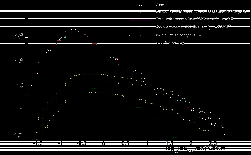
=dX Distribution and Fit Results . . . . . . . . . . . . . . 130

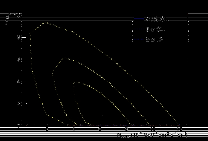
12.2 Upper Limits on Astrophysical Neutrino Fluxes . . . . . . . . . . . . . 132

12.2.1 ?

? 2

. . . . . . . . . . . . . . . . . . . . . . . . . . . . 132

12.2.2 Other Models of Astrophysical Neutrino Fluxes . . . . . . . . . 136

12.3 Measurement of the Atmospheric Neutrino Flux . . . . . . . . . . . . . 140

12.4 Upper Limits on Prompt Atmospheric Neutrinos . . . . . . . . . . . . . 144

13 Conclusions and Outlook

145

13.1 SummaryofResults . . . . . . . . . . . . . . . . . . . . . . . . . . . . 145

13.2 Discussion and Outlook . . . . . . . . . . . . . . . . . . . . . . . . . . 146

A Event Selection Progression

160

vii

B Candidate Neutrino Event Displays

172

C Neutrino E?ective Area Tables

177

D Analysis Sensitivity and Astrophysical ?

Discovery Potential

180

viii

List of Tables

3.1 Critical Energies for Various Particles . . . . . . . . . . . . . . . . . . . 20

3.2 Summary of Charm Particles . . . . . . . . . . . . . . . . . . . . . . . 21

7.1 IceCube 40-string single atmospheric muon live-times . . . . . . . . . . 49

7.2 IceCube 40-string Neutrino Monte Carlo Summary . . . . . . . . . . . 49

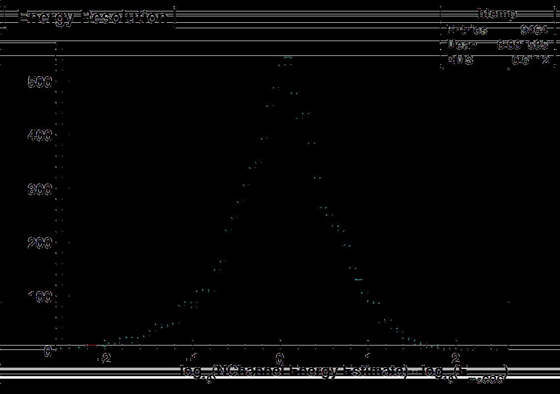
8.1 Energy Resolution for IceCube in the 40 String Con?guration . . . . . 73

8.2 dE

reco

=dX spread for di?erent values of E

for IceCube in the 40 String

Con?guration . . . . . . . . . . . . . . . . . . . . . . . . . . . . . . . . 75

8.3 log

) RMS for two values of dE

reco

=dX for IceCube in the 40 String

Con?guration . . . . . . . . . . . . . . . . . . . . . . . . . . . . . . . . 80

9.1 IceCube 40-string Level-1 Muon Filter . . . . . . . . . . . . . . . . . . 85

9.2 FinalPurityCuts . . . . . . . . . . . . . . . . . . . . . . . . . . . . . . 91

9.3 Data and MC Passing Rates for Successive Purity Cuts . . . . . . . . . 94

11.1 Summary of Nuisance Parameters . . . . . . . . . . . . . . . . . . . . . 126

11.2 Simulated range of scattering and absorption coe?cients . . . . . . . . 127

12.1 FitResults. . . . . . . . . . . . . . . . . . . . . . . . . . . . . . . . . . 130

12.2 Upper Limits for Astrophysical ?

for di?erent Astrophysical Models . 140

12.3 All-?avor (?

+ ?

) Upper Limits for Astrophysical Neutrinos for

di?erent Astrophysical Models . . . . . . . . . . . . . . . . . . . . . . . 140

12.4 Upper Limits on Prompt Atmospheric Neutrinos for di?erent Models . 144

A.1 FinalPurityCuts . . . . . . . . . . . . . . . . . . . . . . . . . . . . . . 161

A.2 Data and MC Passing Rates for Successive Purity Cuts . . . . . . . . . 161

B.1 The four highest energy events in the ?nal analysis sample for the Ice-

Cube40-stringdataset. . . . . . . . . . . . . . . . . . . . . . . . . . . 172

C.1 Neutrino e?ective area for ?

+??

in di?erent zenith ranges . . . . . . . 178

C.2 Neutrino e?ective area for ?

+ ??

over all zenith ranges . . . . . . . . . 179

D.1 Analysis Sensitivity and Astrophysical ?

Discovery Potential . . . . . 180

List of Figures

1.1 The Three Frontiers of Particle Physics . . . . . . . . . . . . . . . . . .

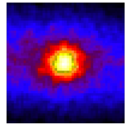
1.2 Image of the Sun in Neutrinos . . . . . . . . . . . . . . . . . . . . . . .

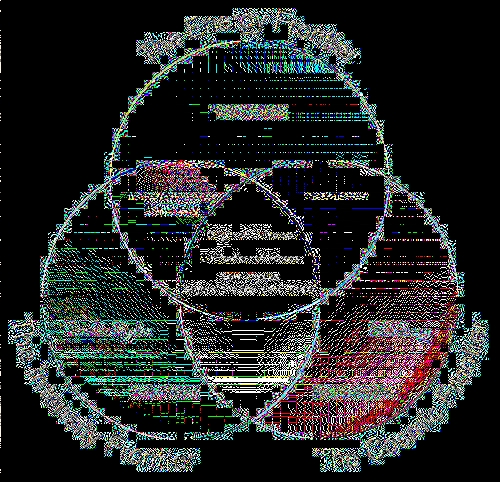
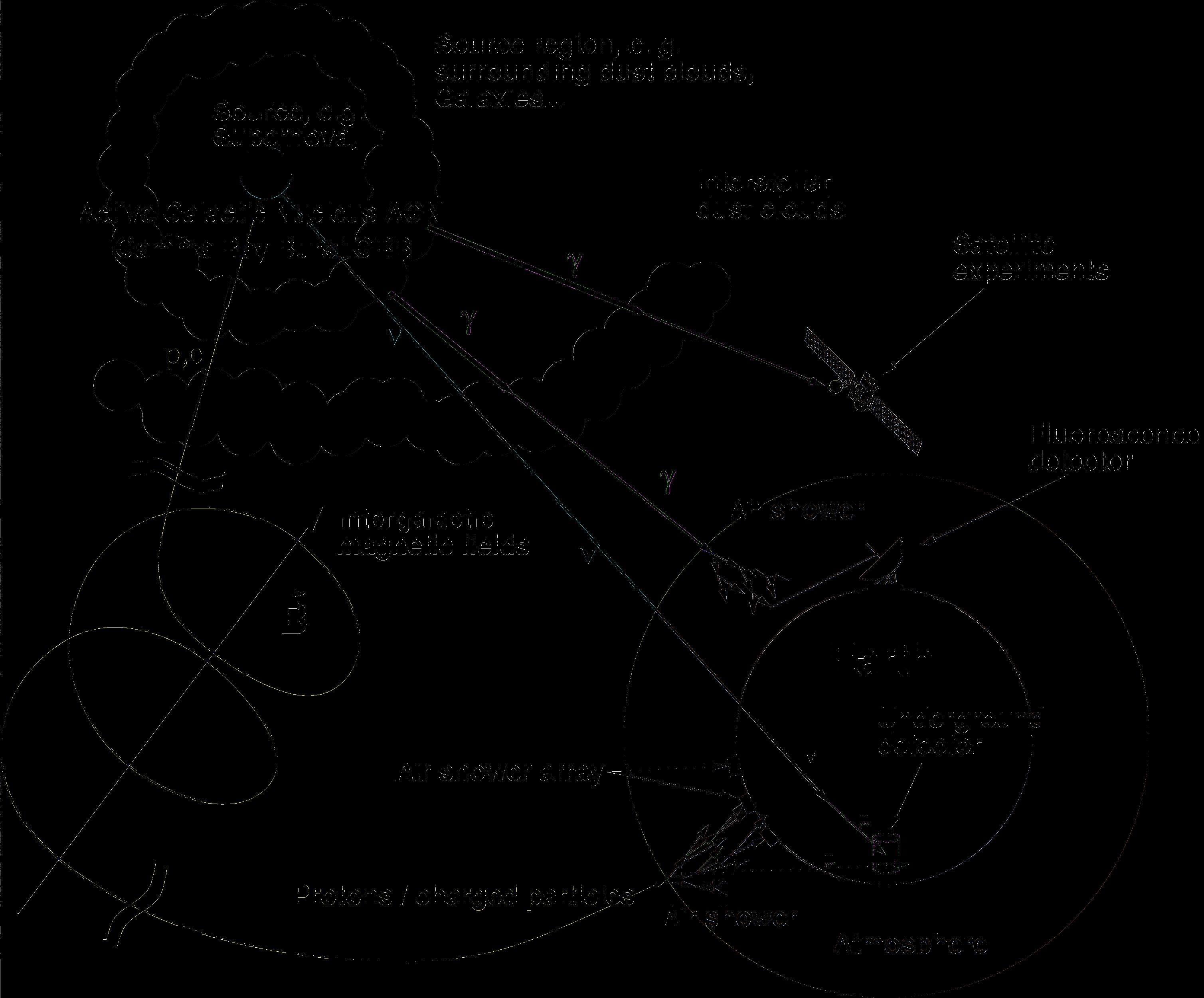
1.3 Neutrinos as Cosmic Messengers . . . . . . . . . . . . . . . . . . . . . .

2.1 The Cosmic Ray Energy Spectrum . . . . . . . . . . . . . . . . . . . .

2.2 Model Predictions for Astrophysical Neutrinos from Unresolved Sources 13

3.1 Schematic of an Extensive Air Shower . . . . . . . . . . . . . . . . . . . 19

4.1 Feynman Diagrams for Neutrino-quark Interactions . . . . . . . . . . . 25

4.2 Neutrino-nucleon Deep Inelastic Scattering Cross Sections . . . . . . . 26

4.3 Cerenk?

ov Cone Geometry . . . . . . . . . . . . . . . . . . . . . . . . . 27

4.4 Average Muon Energy Loss . . . . . . . . . . . . . . . . . . . . . . . . 29

5.1 Schematic of The IceCube Neutrino Observatory . . . . . . . . . . . . . 33

5.2 DigitalOpticalModule . . . . . . . . . . . . . . . . . . . . . . . . . . . 35

6.1 Scattering and Absorption as a Function of Depth . . . . . . . . . . . . 42

7.1 IceCube Monte Carlo Simulation Chain . . . . . . . . . . . . . . . . . . 45

8.1 MuonTrackGeometry . . . . . . . . . . . . . . . . . . . . . . . . . . . 52

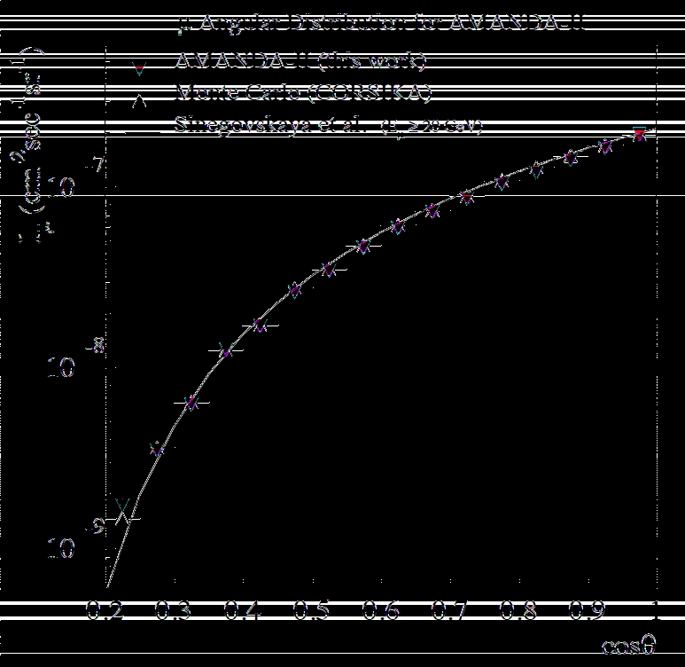
8.2 Angular Distribution of Atmospheric Muons . . . . . . . . . . . . . . . 60

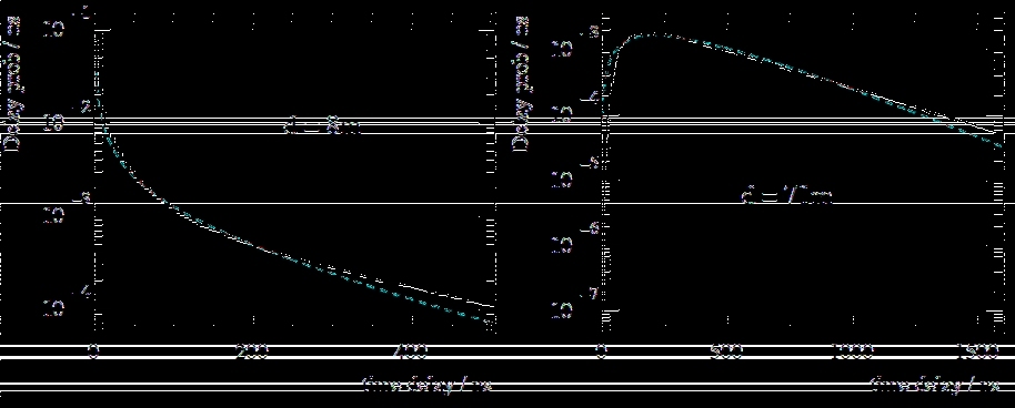
8.3 Time Residual Distribution of the Pandel Function . . . . . . . . . . . 63

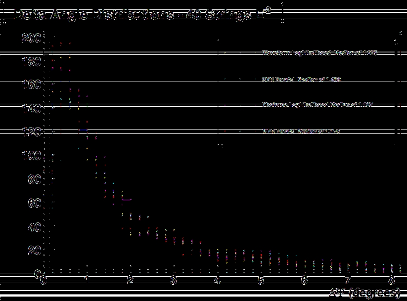
8.4 Angular Resolution of di?erent Muon Track Reconstruction Algorithms 65

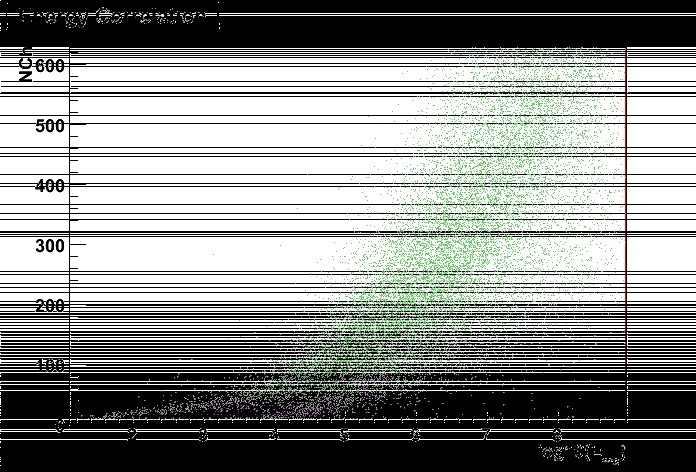
8.5 NChannel Correlation with Muon Energy . . . . . . . . . . . . . . . . . 67

8.6 Photo-electron distribution modeled with the Lightsaber Approximation 68

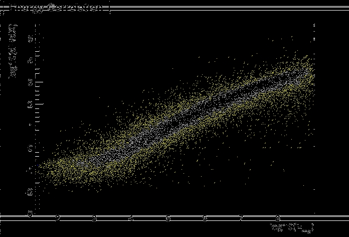
8.7 dE

reco

=dX Correlation with Muon Energy . . . . . . . . . . . . . . . . 70

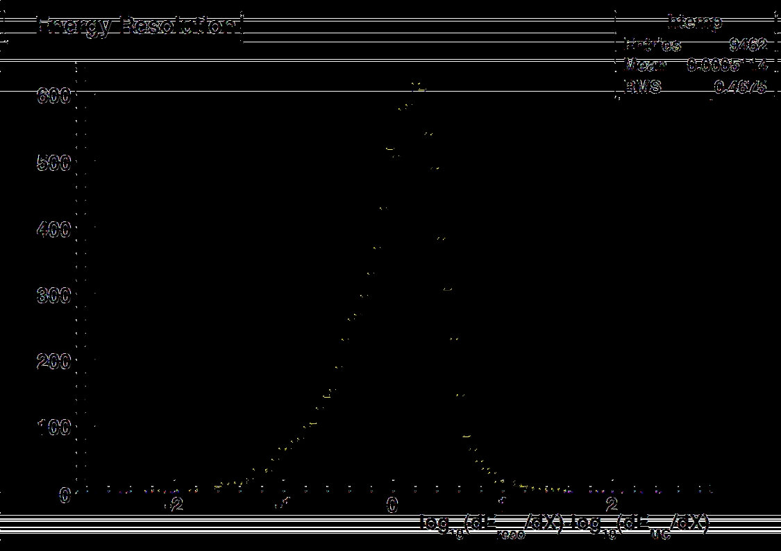
8.8 Energy Estimator Resolution. . . . . . . . . . . . . . . . . . . . . . . . 71

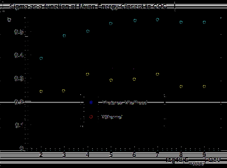
8.9 Energy Estimator Resolution as a Function of Muon Energy . . . . . . 72

8.10 dE

reco

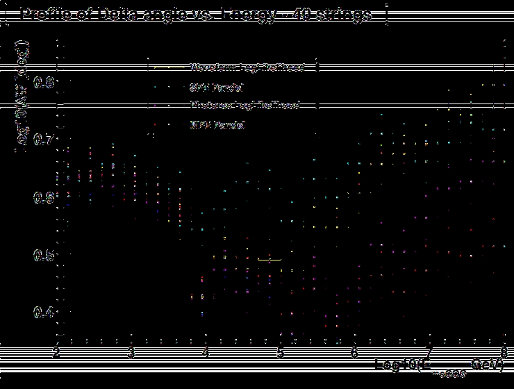
=dX Correlation with Neutrino Energy . . . . . . . . . . . . . . . 74

8.11 Pro?le of the Spread in dE

reco

=dX vs. Neutrino Energy . . . . . . . . . 75

8.12 dE

reco

=dX distribution for 10 TeV Neutrino Energy . . . . . . . . . . . 76

8.13 dE

reco

=dX distribution for 100 TeV Neutrino Energy . . . . . . . . . . 77

8.14 Pro?le of the Spread in Neutrino Energy vs. dE

reco

=dX . . . . . . . . . 78

8.15 E

distribution in di?erent ranges of dE

reco

=dX . . . . . . . . . . . . . 79

9.1 Level 2 Muon Filter Processing Chain . . . . . . . . . . . . . . . . . . . 84

9.2 Filter Level Down-going Muon Background Data-Monte Carlo Com-

parison. . . . . . . . . . . . . . . . . . . . . . . . . . . . . . . . . . . . 87

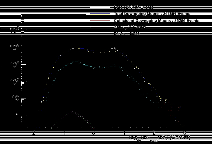
9.3 High Quality Down-going Muon Background dE

reco

=dX distribution . . 92

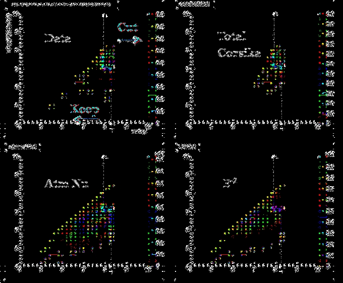
9.4 Cut Progression for dE

reco

=dX and cos(?) . . . . . . . . . . . . . . . . 93

9.5 Analysis Level Data/MC Comparisons for dE

reco

=dX and cos(?) . . . . 96

9.6 Analysis Level Data/MC Comparisons for Physics Observables . . . . . 97

9.7 Analysis Level Data/MC Comparisons for Track Quality Variables . . . 98

9.8 Analysis Level Data/MC Comparisons for Log-likelihood Track Variables 99

xii

9.9 Analysis Level Data/MC Comparisons for Likelihood-ratio test Statistics100

9.10 Analysis Level Data/MC Comparisons for Split-Fit Zenith Angles . . . 101

9.11 IceCube 40-String E?ective Area . . . . . . . . . . . . . . . . . . . . . 102

10.1 Simulated Atmospheric and Astrophysical ?

+ ??

Energy Distribution 104

10.2 Simulated Atmospheric and Astrophysical ?

+??

reco

=dX Distribution105

11.1 Models of the Conventional Atmospheric Neutrino Flux Energy Spectrum115

11.2 Relative Contribution from Pions and Kaons to Atmospheric Neutrinos 116

11.3 Models of the Prompt Atmospheric Neutrino Energy Spectrum . . . . . 118

11.4 dE

reco

=dX Dependence on the Cosmic Ray Slope . . . . . . . . . . . . 119

11.5 dE

reco

=dX Dependence on the Absolute DOM Sensitivity . . . . . . . . 120

11.6 dE

reco

=dX Dependence on the Ice Properties . . . . . . . . . . . . . . . 121

11.7 dE

reco

=dX Dependence on the Muon Energy Loss Cross Sections . . . . 123

11.8 Simulated Contribution of ?

+??

to dE

reco

=dX . . . . . . . . . . . . . 125

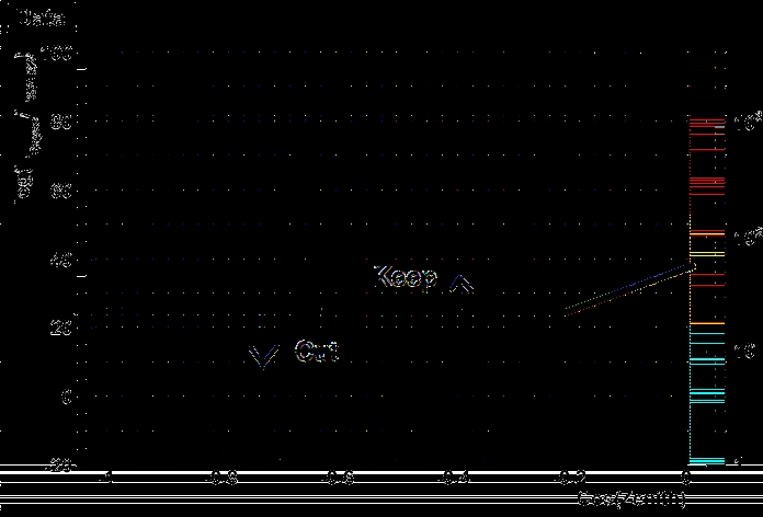
12.1 dE

reco

=dX Fitted to the Data . . . . . . . . . . . . . . . . . . . . . . . 131

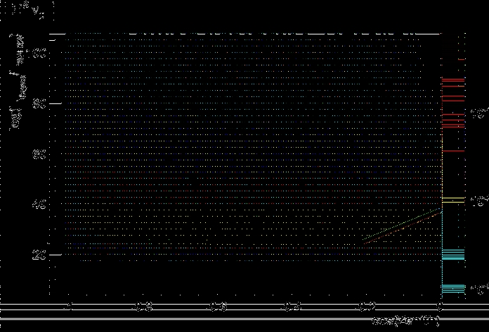
12.2 Allowed Regions for Astrophysical E

? 2

and Prompt Atmospheric ?

133

12.3 Upper Limits on Astrophysical Neutrino ?

Fluxes . . . . . . . . . . . . 134

12.4 Upper Limits on Astrophysical Neutrino Fluxes of all ?avors . . . . . . 135

12.5 Stecker Blazar Model dE

reco

=dX Distribution . . . . . . . . . . . . . . 137

12.6 Becker-Biermann-Rodhe Radio Galaxy Model dE

reco

=dX Distribution . 138

12.7 Mannheim AGN Model dE

reco

=dX Distribution . . . . . . . . . . . . . 139

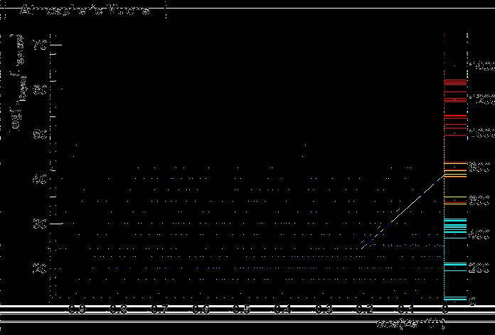
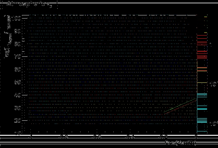
12.8 Allowed Regions for Conventional Atmospheric ?

and ?? . . . . . . . 142

12.9 Measured Atmospheric Neutrino Flux . . . . . . . . . . . . . . . . . . . 143

xiii

13.1 Contribution of ?

to the Prompt Atmospheric Neutrino Flux . . . . . 147

A.1 Filter Level Zenith Distribution . . . . . . . . . . . . . . . . . . . . . . 162

A.2 Reduced Log Likelihood Cut . . . . . . . . . . . . . . . . . . . . . . . . 163

A.3 NDircut. . . . . . . . . . . . . . . . . . . . . . . . . . . . . . . . . . . 164

A.4 Bayesian Likelihood Ratio Cut . . . . . . . . . . . . . . . . . . . . . . . 165

A.5 Split Bayesian Likelihood Ratio Cut . . . . . . . . . . . . . . . . . . . . 166

A.6 ?

splittime

cut . . . . . . . . . . . . . . . . . . . . . . . . . . . . . . . . . 167

A.7 ?

splitgeo

cut . . . . . . . . . . . . . . . . . . . . . . . . . . . . . . . . . . 168

A.8 NDircut. . . . . . . . . . . . . . . . . . . . . . . . . . . . . . . . . . . 169

A.9 LDircut . . . . . . . . . . . . . . . . . . . . . . . . . . . . . . . . . . . 170

A.10SDircut . . . . . . . . . . . . . . . . . . . . . . . . . . . . . . . . . . . 171

B.1 88.7 TeV Muon Candidate Neutrino Event . . . . . . . . . . . . . . . . 173

B.2 103 TeV Muon Candidate Neutrino Event . . . . . . . . . . . . . . . . 174

B.3 107 TeV Muon Candidate Neutrino Event . . . . . . . . . . . . . . . . 175

B.4 185.7 TeV Muon Candidate Neutrino Event . . . . . . . . . . . . . . . 176

D.1 IceCube 40-String Discovery Potential . . . . . . . . . . . . . . . . . . 182

Chapter 1

Introduction

Man has pondered the mysteries of the universe for thousands of years by looking to the

sky. Guided by visible light from stars and other cosmic objects, mankind has learned

much about the universe and our place in it. During the last century, new windows

into the universe were opened using di?erent wavelengths of light revealing new and

unexpected phenomena. A common theme with many of these discoveries is that the

universe is often ferocious and energetic. The universe is still ?lled with light from the

primordial explosion of the Big Bang, matter collides and spirals around supermassive

black holes at the center of galaxies, heavy stars explode in supernova, and even

heavier stars explode and binary systems collide resulting in violent explosions known

as gamma ray bursts.

Under such extreme conditions, scientists use the cosmos as a laboratory to

investigate the fundamental laws of physics from a vantage point that is inaccessible

to even the highest energy particle accelerators on Earth. These new windows to the

universe have not only revolutionized astronomy, but also has opened up a new cosmic

frontier of particle physics that help answer questions in fundamental physics while

also revealing new mysteries. Among these are cosmic rays; high energy protons and

nuclei that are acelerated to energies far beyond what can be achieved by any particle

accelerator on Earth. Cosmic rays bombard Earth continuously and their ultimate

origin is a currently an unsolved problem in astrophysics.

Neutrinos deepen the connection between particle physics and astronomy. Any-

where nuclear reactions or high energy collisions take place, neutrinos are a ?ngerprint

of such interactions. Neutrinos were produced in large numbers right after the Big

Bang [3], in the cores of stars (?g. 1.2), when heavy stars explode in supernova [4],

and other potential celestial objects. The new window to the universe provided by

the neutrino has already revolutionized our understanding of fundamental physics and

the sun. The discovery that neutrinos have mass solved a longstanding problem in

astronomy where fewer neutrinos were observed from the sun than were predicted [5].

Wolfgang Pauli proposed the neutrino in 1933 [6] to solve a known problem where

radioactive beta decay appeared to violate energy conservation. The observation of

the neutrino proved elusive for 20 years until Clyde Cowan and Frederick Reines [7]

?rst detected the anti-social particle coming from the Hanford and Savannah River

nuclear reactors. Neutrinos, having no electric charge and interacting only via the

weak interaction, are ideal cosmic messengers to study the high-energy universe since

they enable physicists to observe environments inaccessible to optical telescopes. (See

?g. 1.3.)

Neutrino astronomy is still new ?eld. The only con?rmed sources of extrater-

restrial neutrinos are from the sun and Supernova SN 1987a. The main goal of the

IceCube Neutrino Observatory is the detection of new sources of high energy astro-

physical neutrinos. The goal of this work is the search for high energy extraterrestrial

Figure 1.1: The three frontiers of particle physics. Research in fundamental physics

progresses on three fronts: the energy frontier, the intensity frontier and the cosmic

frontier. At the energy frontier, physicists build particle accelerators to collide particles

at the highest possible energy in order to create new particles. Physicists at the

intensity frontier use accelerators with intense beams and experiments with very large

volumes to study processes that occur only rarely in nature. Physicists at the cosmic

frontier take insight from the new windows to the universe provided by astronomers

to explore physics inaccessible in a laboratory environment. Taken from [1].

Figure 1.2: Image of the sun in neutrinos, taken by the Super-Kamiokande neutrino

experiment [2]. Image Credit: R Svoboda and K. Gordan

Figure 1.3: The neutrino's role in multi-messenger high energy astrophysics. Cosmic

rays are charged and therefore lose their directional information by the time they ar-

rive at Earth. Gamma-rays have a short horizon and easily absorbed by dust, the

infrared background, and cosmic microwave background. Discrimination between the

production mechanisms responsible for the gamma-rays is also di?cult, since most

gamma-ray sources are equally well described by electromagnetic or hadronic accel-

eration models. Neutrinos are uncharged and only interact via the weak interaction,

making them ideal cosmic messengers for the high-energy universe. Image Credit:

Wolfgang Rhode

neutrinos from unresolved astrophysical sources. The presence of such a di?use ?ux

of astrophysical neutrinos carries a lot of information about the distribution of cosmic

accelerators in the universe, while the lack of such a signal enables us to set strong

constraints on the distribution of such high energy sources.

Chapter 2

High Energy Neutrino Astrophysics

Although neutrino astronomy is still in its infancy, it has great potential to revolu-

tionize our understanding of many astrophysical phenomena. It is in particular well

positioned to elucidate the origin of the high energy cosmic rays whose ultimate origin

remain a mystery since their discovery by Vector Hess's [8] balloon ?ights in 1912. We

shall see that the production of high energy astrophysical neutrinos is closely linked

to the acceleration of high energy cosmic rays in the universe.

2.1 Cosmic Rays

Cosmic rays are high energy charged particles traveling through the universe.

The majority of cosmic rays (79% [9]) are protons while the other 21% of the cosmic

ray composition consists of helium nuclei, (15%), electrons (2%), and elements heavier

than helium (4%). Although the Large Hadron Collider at CERN will accelerate

protons to a center of mass energy of 14 TeV, cosmic rays have been observed with

energies as high as 10

eV making them the highest energy particles ever observed. An

important feature of the cosmic ray energy spectrum is that it follows a power law over

many orders of magnitude in energy. This indicates that cosmic rays can not result

from thermal processes, but instead must come from non-thermal mechanisms which

focus the energy out?ow from a source onto a relatively small number of particles.

The measured cosmic ray spectrum is shown in ?g. 2.1, which shows the results of

both direct measurements from satellite and balloon-based experiments and indirect

measurements from air shower arrays.

The di?erential ?ux is dN=dE / E

? 2 : 7

[9] over many decades in energy until a

feature around 10

eV known as \the knee" where the spectrum steepens to dN=dE /

? 3 : 2

. The exact mechanism responsible for the knee has yet to be understood, but

it has been hypothesized that a rigidity dependent cuto? [11] in the spectrum would

be natural as cosmic rays di?use out of the milky way galaxy at higher energies. The

slope changes again with a feature called \the ankle" at 5 ? 10

eV where the spectrum

hardens back to dN=dE / E

? 2 : 7

. The cosmic ray spectrum gets suppressed above

5 ? 10

eV [12] by the Greizen-Zatsepin-Kuzmin (GZK) mechanism, where cosmic

ray protons are above the energy threshold to interact with the cosmic microwave

background photons to produce pions.

For energies below the knee, shock waves produced by supernova remnants in

the milky way galaxy [13] provide natural non-thermal candidates to accelerate cosmic

rays. As the cosmic ray spectrum transitions from galactic to extra-galactic in origin

at higher energies above the knee, larger acceleration sites and stronger magnetic ?elds

are necessary to explain the observed energies. Natural extragalactic source candidates

include active galactic nuclei and gamma ray bursts.

-10

-8

-6

-4

-2

dN/dE (GeV cm

-2

-1

)

kin

(GeV / particle)

Energies and rates of the cosmic-ray particles

protons only

all-particle

electrons

positrons

antiprotons

CAPRICE

BESS98

AMS

Grigorov

JACEE

Akeno

Tien Shan

MSU

KASCADE

CASA-BLANCA

DICE

HEGRA

CasaMia

Tibet

AGASA

HiRes

Auger

Figure 2.1: The cosmic ray energy spectrum as measured from di?erent experiments.

The cosmic ray ?ux has been multiplied by E

to enhance features. Taken from [10].

2.2 Astrophysical Neutrino Production

Active galactic nuclei (AGN), gamma ray bursts (GRBs), and supernova rem-

nants (SNR) are among the leading candidate astronomical objects that could accel-

erate cosmic rays to high energies and produce neutrinos. As mentioned in the last

section, the power law nature of the cosmic ray spectrum indicates a non-thermal

mechanism is responsible for their acceleration. A widely held non-thermal accelera-

tion mechanism due to magnetic shocks is ?rst order Fermi acceleration [14]. Charged

particles are con?ned to the shock region by magnetic inhomogeneities and are there-

fore continuously accelerated by repeated magnetic de?ection through the shock front.

First order Fermi acceleration predicts a primary cosmic ray spectrum of:

/ E

? 2

(2.1)

With high densities of matter and radiation at the source, the accelerated cos-

mic ray primaries may interact and not escape. Neutrinos are produced from the

hadronic nucleon-photon and nucleon-nucleon interactions in the astrophysical shock

fronts which result in the production of pions. Pion production occurs via the delta

resonance for nucleon-photon interactions and the dominant channels are:

p? ! ?

! p+ˇ

(2.2)

! n+ˇ

n? ! ?

! n+ˇ

(2.3)

! p+ˇ

The dominant pion-production channels for nucleon-nucleon scattering are:

pp ! p+p+ˇ

p+n+ˇ

pn ! p+n+ˇ

(2.4)

p+p+ˇ

It can be seen that half of the pions produced are charged where as the other

half are neutral. The charged pions decay to produce neutrinos and the neutral pions

decay into gamma rays:

! ?

(2.5)

! e

+??

! ?

+??

(2.6)

! e

+??

! ??

(2.7)

At higher energies, kaons can also be produced [15] and contribute to the neutrino

and gamma ray ?ux. The resulting neutrinos and gamma rays follow the energy

spectrum of the primary cosmic rays. Astrophysical neutrinos and gamma rays from

hadronic interactions are therefore predicted to have a dN=dE / E

? 2

energy spectrum.

The neutrino ?ux at the source has a ?avor ratio of

: ?

= 1 : 2 : 0

(2.8)

Neutrinos have a small but non-zero mass, which causes them to oscillate and

change ?avors. The expected ?avor ratio of astrophysical neutrinos at Earth is [16]:

: ?

= 1 : 1 : 1

(2.9)

Although the particle physics responsible for the production of neutrinos and

gamma rays is well known, the underlying astrophysical details are poorly understood.

We consider several models for astrophysical neutrinos in the next section.

2.3 Astrophysical Neutrino Models

Neutrino astrophysics is a young ?eld. With the underlying astrophysics respon-

sible for the hadronic acceleration of cosmic rays being so uncertain, a wide range of

models have been developed to calculate the neutrino ?ux from di?erent astrophysical

source classes. These models generally use a particular waveband (radio, cosmic rays,

gamma rays) to determine the normalization of the neutrino ?ux. This work searches

for an isotropic distribution of astrophysical muon neutrinos from unresolved sources.

The models considered in this analysis calculate the total sum of astrophysical neu-

trinos from di?erent extragalactic source classes that contribute to a di?use ?

?ux.

These models are shown in ?g. 2.2 and are described in this section.

[GeV]

log

-1

-2

GeV cm

/dE

-9

-8

-7

-6

-5

-4

-3

Razzaque GRB Progenitor 2003

Waxman Bahcall Prompt GRB

Blazars Stecker 2005

Waxman Bahcall 1998 x 1/2

Becker-Biermann-Rodhe FSRQ 2005

BL LACs Mucke et al 2003

Mannheim AGNs 1995

Engel-Seckel-Stanev Cosmogenic Neutrinos 2001

Figure 2.2: Di?use astrophysical neutrino model predictions for di?erent extraterres-

trial source classes. The models for active galactic nuclei include predictions from

Stecker [17], Muc? ke et al. [18], Becker-Biermann-Rodhe [19], and Mannheim [20]. The

two models for gamma ray bursts shown are described by Razzaque and Meszaros

in [21]. An upper bound on astrophysical neutrinos is calculated by Waxman and

Bahcall in [22]. Finally, neutrinos produced by the GZK suppression of the cosmic ray

?ux is calculated by Engel, Seckel, and Stanev [23].

2.3.1 Waxman-Bahcall Upper Bound

The Waxman-Bahcall upper bound [22] assumes that the extragalactic cosmic

ray ?ux has a ? / E

? 2

spectrum. Consistent with the observed cosmic ray spectrum,

an energy production rate for protons was assumed to be

dN_

= 10

erg Mpc

? 3

? 1

(2.10)

An upper bound on the astrophysical neutrino ?ux was derived for optically thin

sources. Since half of the produced pions are charged and half the energy of the charged

pions goes into the muon neutrinos, the upper bound on the di?use astrophysical

neutrino ?ux is given by

=0:25 t

? E

dN_

(2.11)

The Hubble time, t

= 10

years, is given by the inverse of the Hubble constant

which was assumed to be H = 65 km s

? 1

Mpc

? 1

in the calculation. The upper bound

on the ?ux was calculated to be 1:5 ? 10

? 8

GeV cm

? 2

? 1

. After correcting for

redshift evolution and neutrino oscillations, the upper bound for muon neutrinos at

Earthis2:25 ? 10

? 8

GeV cm

? 2

? 1

2.3.2 Becker, Biermann, and Rhode Radio Galaxy Model

Becker, Biermann, and Rhode [19] calculated the di?use astrophysical neutrino

?ux from active galactic nuclei using observations from FR-II radio galaxies. The

jet of the AGN is a candidate site for p + ? interactions and subsequent photo-pion

production. The observations from FR-II radio galaxies was used to normalize the ?ux

of neutrinos by assuming a relationship between the disk luminosity, the luminosity

in the observed radio band, and the calculated neutrino ?ux. ? / E

? 2

was assumed

for the proton energy spectrum in the model considered in this work.

2.3.3 Astrophysical Neutrinos from Blazars

For optically thick sources, TeV gamma rays that are produced from the decay

of neutral pions cascade to lower energies resulting in the emission of sub-TeV pho-

tons. The observed di?use extragalactic gamma ray ?ux from the experiments in the

Compton Gamma Ray Observatory satellite can therefore be interpreted as hadronic

gamma-rays avalanched to lower energies. The neutrino ?ux can therefore be nor-

malized to the di?use extragalactic gamma-ray background detected by the EGRET

and COMPTEL experiments that were onboard the Compton Gamma Ray Observa-

tory. These two experiments were sensitive in di?erent energy ranges, with EGRET

detecting a di?use extragalactic gamma-ray ?ux at higher energies (E

> 100 MeV)

and COMPTEL measuring the di?use component at lower energies (E

< 100 MeV).

A model of p + ? interactions and p + p collisions at the core of AGNs is derived by

Mannheim [20] which uses the EGRET di?use observation to normalize the neutrino

?ux calculation. The model calculated by Stecker [17] uses the results from COMP-

TEL to normalize the neutrino ?ux resulting from pp and p? interactions at the core

of the blazar.

2.3.4 High-Frequency Peaked BL-LACs Model

BL-LACs that are observed to emit TeV gamma rays can be interpreted to be

optically thin to photon-neutron interactions. The model calculated by Muc? ke et

al. [18] assumes that charged cosmic rays are produced in these sources through the

decay of escaping neutrons. The resulting neutrino ?ux would be proportional to the

observed extra-galactic cosmic ray ?ux at Earth. The calculation of the neutrino ?ux

connects the observed cosmic ray ?ux to TeV emission from high frequency peaked BL-

LACs. The ?ux is calculated to be quite small and peaks at high energies (10

GeV).

2.3.5 Neutrinos from Gamma-Ray Bursts

Gamma-Ray Bursts are the highest energy explosions known in the universe with

energies greater than 10

erg over an extremely short time scale of 10

? 3

s ? 1000 s.

They are a prime candidates to accelerate the highest energy cosmic rays. The non-

thermal emission occurs in three stages: the precursor phase hours before the GRB, the

prompt phase coincident with the burst, and the afterglow phase. Although there is a

wide variation in gamma-ray burst emission pro?les, an average spectrum of neutrinos

from the precursor and prompt phases of GRBs is calculated in [21] by correlating the

gamma-ray emission to the observed ?ux of ultra high energy cosmic rays.

2.3.6 Cosmogenic Neutrinos

The observation of the GZK suppression in the cosmic ray ?ux above the ankle

implies the existence of a high energy astrophysical neutrino ?ux. It is called one of

the guaranteed sources of neutrinos induced by the cosmic ray ?ux, with the other

two being neutrinos produced by the propagation of cosmic rays through plane of the

milky way galaxy and atmospheric neutrinos which are described in the next chapter.

The cosmogenic neutrino ?ux, which has yet to be observed, originates from the GZK

mechanism of photo-pion production by protons interacting with the cosmic microwave

background. A calculation of the cosmogenic ?ux is done by Engel, Seckel, and Stanev

in [23].

2.3.7 Other Sources of High Energy Astrophysical Neutrinos

Not considered in this work are other sources of high energy astrophysical neu-

trinos. Among these models are neutrinos from the decay of exotic relic particles [24]

and neutrinos from the annihilation of neutralino dark matter [25].

Chapter 3

Atmospheric Neutrinos

3.1 Neutrino Production in Extensive Air Showers

The primary background in a search for high energy astrophysical neutrinos is

the atmospheric neutrino and muon background produced in the Earth's atmosphere.

High energy cosmic rays interact with air molecules in the Earth's atmosphere which

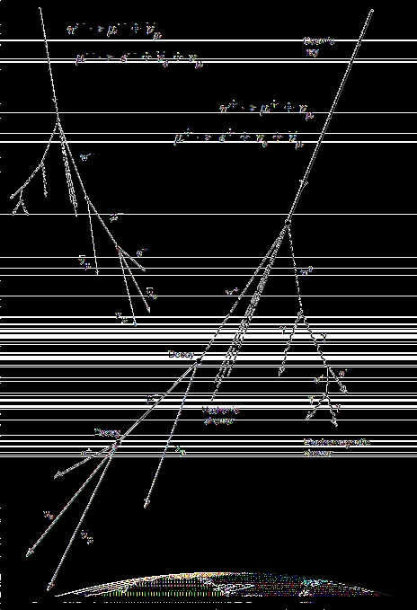
results in a cascade of particle production and decay. This chain leads to an extensive

air shower of electrons, positrons, pions, kaons, muons, and neutrinos. In quite an

analogous manner to the astrophysical production of neutrinos discussed in the last

chapter, atmospheric neutrinos are produced through the hadronic interactions of

cosmic ray primaries with the atmosphere generating charged pions and kaons, which

subsequently decay into muons and muon neutrinos:

! ?

(3.1)

! ?

+??

Figure 3.1: An extensive air shower leading to the production of atmospheric muons

and neutrinos. Taken from [26]

An example of an extensive air shower is shown schematically in ?g. 3.1. Some

of the muons produced in the shower would decay producing both electron and muon

neutrinos according to eq. 2.5 and eq. 2.6. The atmospheric neutrino ?ux due to the

decay of pions and kaons are commonly referred to as the conventional atmospheric

neutrino ?ux.

While the ?ux of the parent cosmic ray primaries is isotropic, the conventional

atmospheric neutrino ?ux has a complicated zenith angle dependence due to the kine-

matics of meson interaction and decay in the atmosphere. The kinematics of meson

interaction and decay also a?ects the energy spectrum of the atmospheric neutrino

?ux. An important parameter is the critical energy E

crit

which is de?ned as the

energy where the decay length and the interaction length are equal and is de?ned as:

crit

c˝

(3.2)

Table 3.1: Critical energies for various particles. Data from [27].

Particle Constituent Quarks mc

(GeV) E

crit

(GeV )

lepton

0:106

1:0

; ˇ

ud;? ud?

0.140

115

; K

us;? us?

1.116

850

were ˝ is the live-time of the particle and h

comes from the assumption of an

isothermal atmosphere [28]. A lepton or a meson with energies above the critical

energy will more likely interact than decay. Table 3.1 summarizes the critical energies

of the particle types that contribute to the conventional atmospheric neutrino ?ux.

We note that the muon has a critical energy of 1:0 GeV, which is well below the

energy threshold of the IceCube Neutrino Observatory and the sensitivity of this work.

Since the ?

component of the conventional atmospheric neutrino ?ux arises from the

decay of atmospheric muons, the atmospheric electron neutrino ?ux is an order of

magnitude smaller than the ?

?ux in the GeV ? TeV energy range [29]. For energies

below E

crit

, the atmospheric neutrino spectrum follows the primary cosmic ray energy

spectrum. Above the critical energy, the energy spectrum of neutrinos decreases by

one additional power of the energy [29]. Detailed three-dimensional calculations of the

energy spectrum and angular distribution of the conventional atmospheric neutrino

?ux are summarized in [30] and [31].

3.2 Prompt Atmospheric Neutrinos

Table 3.2: Summary of Charm Particles. Data from [27].

Particle Constituent Quarks mc

(GeV) E

crit

(GeV)

; D

cd;? cd?

1:87

3:8 ? 10

; D?

cu;? cu?

1:865

9:6 ? 10

cs;? cs?

1:969

8:5 ? 10

udc

2:285

2:4 ? 10

If the energy of the primary cosmic ray is high enough, the extensive air shower

will include the production and decay of charm baryons and mesons. Charm particles

typically have very short live-times, so the atmospheric neutrino ?ux arising from the

decay of charmed mesons is often called the prompt component of the atmospheric

neutrino ?ux. The charm particles thought to be produced in extensive air showers

are summarized in Table 3.2. The dominant contribution to the prompt ?ux is the

semi-leptonic decay modes of D mesons decaying to Kaons and leptons:

D ! K +l+?

(3.3)

The most common semi-leptonic decay channels are from D

which have a

branching ratio of 17:2% [32]:

! K?

(3.4)

! K

+??

! K?

(3.5)

! K

+??

Since the critical energies (Table 3.2) of charm particles are so high, they will

decay before interacting and subsequently follow the primary cosmic ray energy spec-

trum and have an isotropic angular distribution. We note that the prompt component

of the atmospheric neutrino ?ux has an equal contribution from ?

and ?

. Full cal-

culations of the prompt component of the atmospheric neutrino ?ux are given in [33],

[34], and [35].

3.3 A Comment on Neutrino Oscillations

If neutrinos have a nonzero mass, their mass eigenstates do not correspond to the

?avor eigenstates. This implies that neutrinos can change ?avor as they propagate. A

produced in the atmosphere may appear in the detector as another ?avor. For the

case of two-?avor oscillations (?

and ?

), the survival probability of a muon neutrino

in the atmosphere for the two-?avor oscillation case is [27]:

! ?

= 1 ? sin

(2?

atm

)sin

atm

(3.6)

where ?m

atm

is the squared mass di?erence between the two mass eigenstates

and the baseline L is in natural units of GeV

? 1

. For energies above 50 GeV, atmo-

spheric neutrino oscillations cease for baselines equal to the diameter of the Earth.

Atmospheric neutrino oscillations are therefore unimportant for the majority of anal-

yses done with the IceCube Neutrino Observatory and this work in particular.

Chapter 4

Principles of Neutrino Detection

The small interaction cross section of the neutrino presented a major challenge to

understanding their properties and to the development of neutrino astrophysics. Neu-

trino detectors in general and neutrino telescopes in particular must encompass an

enormous volume to compensate for such low interaction cross sections. The design

of a high energy neutrino telescope involves the use of natural bodies of water or

transparent ice as target material and a detection medium for neutrinos to interact

in. The medium is instrumented with photomultiplier tubes to detect the products of

the neutrino interaction occurring in or near the instrumented detector volume.

4.1 Neutrino-Nucleon Interactions

Neutrinos only interact via the weak interaction. They interact via charged-

current (CC) interactions which are mediated by W

bosons or neutral current (NC)

interactions which are mediated by Z

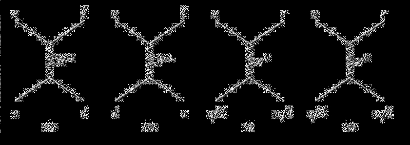
bosons. The Feynman diagrams depicting these

interactions are summarized in ?g. 4.1. A charged-current interaction of a neutrino

with nucleus in the ice produces a charged lepton:

Figure 4.1: Feynman diagrams for neutrino-quark Charged Current and Neutral Cur-

rent interactions

+q ! l+q

(4.1)

where q is a valence or sea quark in the nucleus and q

is a quark of a di?erent

?avor. (The ?avor of the quark is changed by the exchange of a W boson.) As an

example, a muon neutrino that undergoes a charged-current interaction with one of

the ice nuclei would result in a muon.

The deep-inelastic scattering cross sections are the most important for the energy

range relevant to an astrophysical neutrino observatory. The neutrino in the deep-

inelastic regime has enough energy to interact with the quarks or gluons as point

particles. The neutrino transfers enough energy to the parton (a quark or gluon

constituent of the nucleon) such that the interaction dissociates the parent nucleon.

The NC and CC neutrino-nucleon deep inelastic cross sections in ice are summarized

in ?g. 4.2.

Figure 4.2: Charged Current and Neutral Current cross sections for neutrino-nucleon

deep inelastic scattering. From [36], which uses the Parton Distribution Functions

parametrized in CTEQ5. [37]

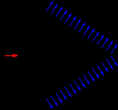
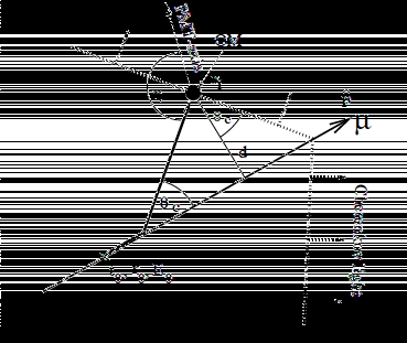
Figure 4.3: Cerenk?

ov cone geometry formed by a relativistic muon traveling through

a medium

4.2 Cerenk?

ov Radiation

Neutrinos can not be seen directly in a detector since they only interact via

the weak interaction. A relativistic muon from a charged-current neutrino-nucleon

interaction radiates light via the Cerenk?

ov e?ect if the muon travels faster than the

speed of light in the medium. The detection of Cerenk?

ov radiation in a transparent

medium arising from neutrino interactions is the primary operating principle of a

neutrino telescope. A coherent front of light analogous to a shock wave forms at a

characteristic angle ?

which depends on the index of refraction of the medium:

cos?

(4.2)

where ? = v=c is the velocity of the particle. The geometry of the Cerenk?

cone is depicted in ?g. 4.3. The Cerenk?

ov angle for ice is ?

c;ice

ˇ 41

for relativistic

particles (? ˇ 1) and an index of refraction n

ice

ˇ 1:33.

The number of Cerenk?

ov photons emitted per unit track length as a function of

wavelength of light ? is given by the Frank-Tamm formula [27]:

dxd?

2ˇ?

1 ?

(4.3)

where ? is the ?ne structure constant. High frequency radiation dominates the

Cerenk?

ov emission due to the 1=?

dependence of the Frank-Tamm formula. A cuto?

at the ultraviolet end of the spectrum is imposed (300 nm [38]) due to the absorption

of light by the glass of the photomultiplier-tube.

4.3 Muon Energy Loss

It is of critical importance to understand the physical processes involved in muon

propagation and energy loss since all information about the atmospheric ?

?ux and

a potential astrophysical ?

?ux is inferred from the secondary muons. Muons do not

lose much energy via Cerenk?

ov radiation, which is estimated to be 24 keV=cm for

> 1 GeV [40]. The muon energy loss rate as a function of distance, dE=dX, is

commonly expressed [27] as:

=a(E)+b(E)E

(4.4)

Where a(E) corresponds to continuous muon energy loss mechanisms and b(E)

corresponds to the sum of stochastic energy losses. An assumption is often made that

a and b are constant such that one can use the relation

ioniz

brems

photo

epair

decay

energy [ GeV ]

energy losses

[

GeV/(g/cm

)

]

-10

-9

-8

-7

-6

-5

-4

-3

-2

-1

1 10 10

Figure 4.4: Average muon energy loss in ice as a function of the energy of the muon.

From [39]

ˇ a+bE

(4.5)

to make an estimate of the energy loss for high energy muons. In ice:

a = 0:25958 GeV=mwe

(4.6)

b = 3:5709 ? 10

? 4

GeV=mwe

with a systematic error of 3:7% [ ? ]. An example of such a calculation is an

estimate of the muon range. The mean range R of a muon with initial energy E

given by integrating eq. 4.5:

R ˇ (1=b) ln

crit

(4.7)

Where E

crit

= a=b is an estimate of the critical energy where continuous and

stochastic energy losses are equal. In ice, E

crit

ˇ 727 GeV. A 1 TeV muon for example

would have a mean range in ice of R ˇ 2:6 km. This illustrates that a muon can have

a range larger than the instrumented volume of a neutrino telescope, so a CC ?

interaction does not need to be contained within the ?ducial volume of the detector.

The continuous and stochastic energy losses of the muon come from di?erent

physical processes. Continuous energy losses come from ionization and stochastic

energy loss mechanisms come from e

pair production, bremsstrahlung, and photo-

nuclear interactions. The energy losses from these various components are shown in

?g. 4.4.

Stochastic muon energy losses in ice come in the form of relativistic electromag-

netic and hadronic showers which also produce visible light due to Cerenk?

ov radiation.

The total light output of a stochastic shower can be estimated from the muon track

length subtended by the constituent particles of the shower. This e?ective track length

has been parameterized with shower energy in ice by C. Wiebusch [41]:

eff

(E) =0:894

( GeV )

? 4:889

For EM showers

(4.8)

eff

(E) =0:860

( GeV )

? 4:076

For Hadronic Showers

The amount of Cerenk?

ov light emitted by a stochastic shower is then calculated

by:

?;S

eff

(E) ? n

(4.9)

where l

eff

(E) is given by eq. 4.8 and n

is obtained by integrating the Frank-

Tamm formula (eq. 4.3) over the sensitivity range of the photomultiplier tube.

Chapter 5

The IceCube Neutrino Observatory

The IceCube Neutrino Observatory is the largest neutrino detector built to date. When

construction is completed in 2011, it will encompass a cubic-kilometer of instrumented

Antarctic ice. The large instrumented volume is necessary because of the low neutrino

interaction cross sections and the low predicted ?ux rates for astrophysical neutri-

nos. The IceCube detector is speci?cally designed to be a large tracking calorimeter,

measuring energy deposition in the form of Cerenk?

ov light contained within the in-

strumented volume.

Neutrino detection in the Antarctic ice was pioneered by AMANDA[42], the

prototype and proof-of-principle for the IceCube detector. Operational from 1996 to

2009, the AMANDA array consisted of 677 optical modules deployed on 19 strings at

a depth between 1900 m and 2000 m. IceCube will be over two orders of magnitude

larger than its predecessor and will use improved electronics.

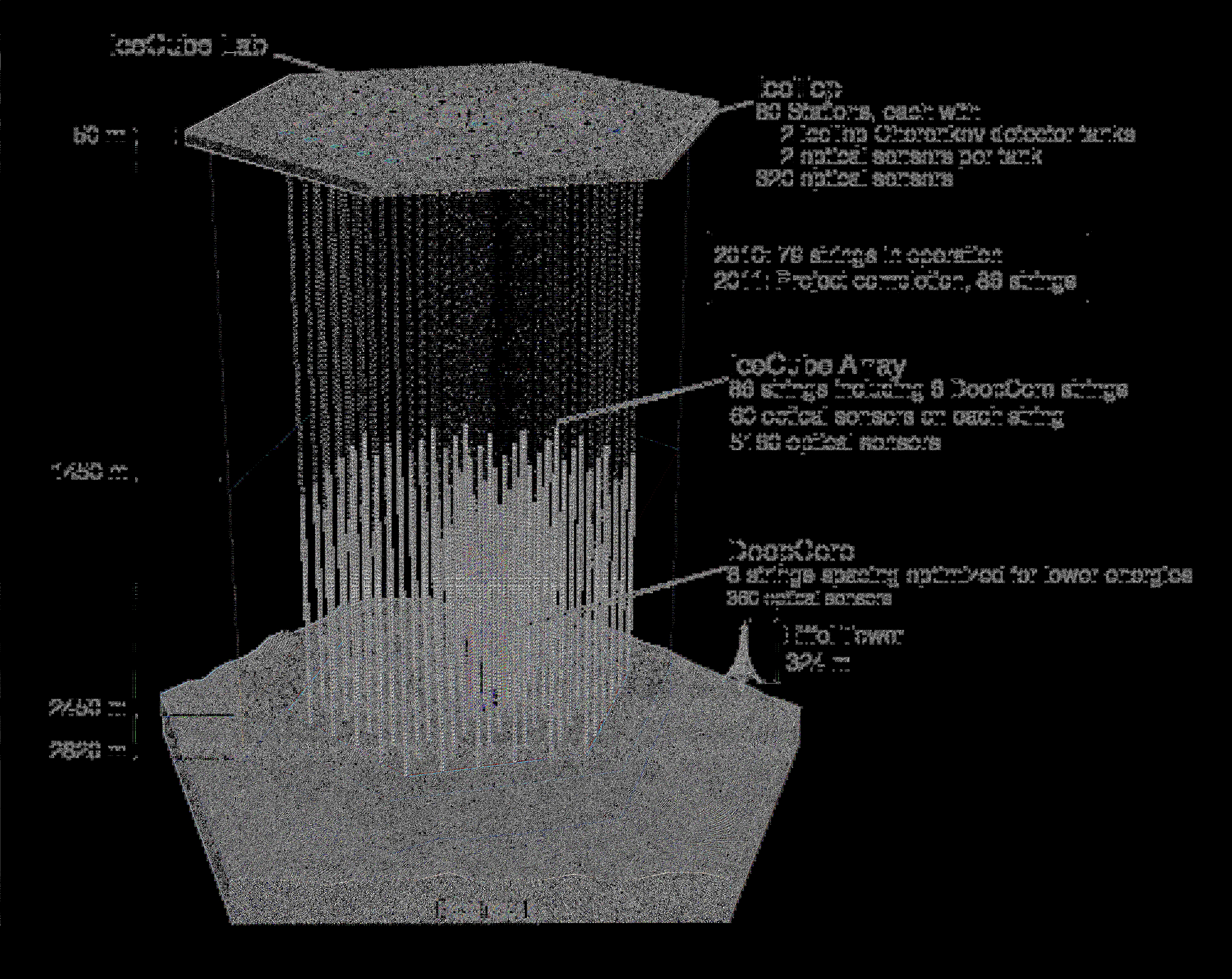
The IceCube design consists of three detectors operating in union, see ?g. 5.1.

The main in-ice array will be composed of 4800 photosensors arranged in 80 strings

which are deployed vertically with 60 photosensors per string. The detector is deployed

deep in the Antarctic ice between a depth of 1450 and 2450 meters. Each photosensor

Figure 5.1: The IceCube Neutrino Observatory

is vertically spaced 17 m from its neighbor and each string of photosensors has a

horizontal spacing of 125 m giving a total instrumented volume of 1 km

. The design

is optimized for the energy range of 100 GeV to 100 PeV [38] and for the event

reconstructions discussed in chap. 8.

The DeepCore extension is deployed within the main in-ice array and consists

of six specialized strings of photosensors with increased quantum e?ciency in order

to lower the energy reach to 10 GeV. Each DeepCore string also has 60 photosensors,

but the extension is more densely spaced than the main in-ice array with a horizontal

spacing of 72 m. Ten of the photosensors are deployed at shallow depths between

1750 m and 1850 m with a 10 m vertical spacing and the other 50 sensors are deployed

with a 7 m vertical spacing at a depth below 2100 m where the Antarctic ice is the

clearest. This extends the number of strings in the main in-ice array to 86 giving

a total of 5160 photosensors. The physics goals of DeepCore include indirect dark

matter searches and atmospheric neutrino oscillations studies [43].

The IceTop surface array [44] is an extensive air shower detector instrumenting

a 1 km

area at the surface of the South Pole directly above IceCube. It will consist

of 160 tanks deployed in pairs with two photosensors per tank. The primary physics

goals of IceTop include measurements of the cosmic ray energy spectrum & mass

composition near the region of the knee and studies of cosmic ray anisotropy.

79 of the total 86 strings are currently operational. The remaining seven strings

will be deployed during the 2010-2011 South Pole construction season. This work is

based on one year of data taken with the 40-string con?guration of IceCube which was

operational from April 2008 to May 2009.

5.1 Digital Optical Modules

Photosensors are critical to the design and construction of a neutrino telescope

since they are responsible for converting Cerenk?

ov light to electrical signals. In the

IceCube Neutrino Observatory, the fundamental photosensor component takes the

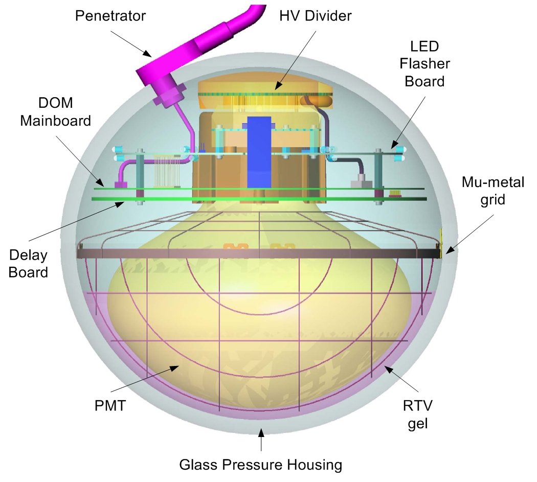
form of a Digital Optical Module (DOM) [45]. Each DOM consists of a 10-inch (25

cm) Hamamatsu photomultiplier tube (model R7081-02) and associated electronics.

These electronics include a 2kV high voltage power supply, a DOM main board, a

delay board, and a LED ?asher board. These components are responsible for the

operation and control of the PMT as well as ampli?cation, ?ltering, and calibration.

The PMT, associated electronics, and mu-metal magnetic shield are housed within

a 35.6 cm pressurized glass sphere. The photocathode glass of the PMT rests in a

silicone gel in order to provide optical coupling to the glass sphere. The DOM is

schematically shown in ?g. 5.2.

Figure 5.2: Schematic of the Digital Optical Module (DOM)

The PMT is sensitive in the wavelength range of 300 nm to 600 nm. The peak

quantum e?ciency of the PMT is 0.25 at around 400 nm and starts to plummet at

shorter wavelengths due to the absorption of UV light by the photocathode glass. It

has ten dynodes and operates in the voltage range between 1200 V and 1400 V with

a gain of 10

The ?asher boards contain twelve LEDs each pointing radially outward. Six of

the LEDs point in the horizontal direction and six point upward at a 48

angle. These

?ashers are useful for timing & geometry calibration, setting the energy scale for an

energy reconstruction, and measurement of the optical properties of the South Pole

Ice.

5.2 Data Acquisition System

Analog waveforms captured by the Hamamatsu PMTs are digitized in situ by the

DOM main board. The analog waveform is ?rst split between a trigger discriminator

and the 75 ns delay board. If the discriminator threshold (0.25 photoelectrons) is

surpassed, the raw waveform is then digitized in two ways.

An Analog Transient Waveform Digitizer (ATWD) digitizes the waveform into

128 bins at a sampling frequency of 300 MHz in order to capture the precise timing

information of the analog signal in a 422 ns long digitized waveform. The ATWD

has three channels operating at three di?erent gains (0.25x, 2x, and 16x) that cover

a dynamic range up to 400 PE/15 ns. A fourth ATWD channel is implemented for

a variety of uses including an internal clock, local coincidence trigger conditions, and

communications. In order to minimize dead time during a trigger readout, two ATWD

chips were designed into the DOM main board. The second method uses a fast Analog

to Digital Converter (fADC) to capture longer waveforms. The 256 bins in the fADC

are sampled at 40 MHz which gives a waveform that is up to 6.4 ?s wide.

A single cable from the surface connects the 60 DOMs in a string to a surface

junction box. (The junction box also receives input from two IceTop tanks.) The

surface junction box provides power ( ? 48 V DC) to the DOMs and relays the acquired

data to the central counting house in the IceCube Laboatory (ICL). Each string is

controlled by a specialized computer in the ICL called a DOMHub. Each DOMHub

contains eight DOM readout (DOR) cards. The DOR card controls the power, boot-

up, software, ?rmware updates, calibration, data transfer, and time calibration of the

DOMs.

The DOMs can operate in local coincidence (LC) mode in order to reduce the

dark noise trigger rate of 540 Hz. DOMs can transmit and receive LC tags to and

from the neighboring vertical DOMs. When a DOM triggers, it transmits a LC tag

to its immediate vertical neighbors and sets a time window of 1 ?s. A DOM satis?es

the LC condition If it receives a reciprocal tag from its vertical neighbor. Hard local

coincidence was implemented for the 40-string con?guration where only waveforms

from DOMs that pass the LC condition are digitized and sent to the surface. Soft

Local Coincidence is also possible where only limited timing information is sent for

waveforms that do not satisfy the LC condition. Soft Local Coincidence (SLC) was

?rst implemented for the 59-string con?guration. The hard local coincidence condition

reduces the false trigger rate to less than 1 Hz. For the 40-string data run, the event

is then sent to a bu?er for further ?ltering (ch. 9) if it passes a simple majority trigger

(SMT) of eight triggered DOMs within a 5 ?s time window.

Chapter 6

Optical Properties of the South Pole Ice

IceCube functions as a neutrino observatory by measuring the Cerenk?

ov light emitted

by relativistic muon tracks and showers. It is therefore extremely important to under-

stand the propagation of Cerenk?

ov photons through the detector medium, which for

IceCube means a thorough understanding of the optical properties of the South Pole

Ice. The ice at the South Pole has a complex depth structure consisting of horizontal

ice sheets with varying degrees of dust concentration [46]. The glacial ice under the

South Pole was created over a period of 165,000 years and currently has a thickness of

2820 m. The ice structure varies quite strongly with depth due to the accumulation

of dust particles due to varying atmospheric conditions and volcanic activity during

the glacial history of Antarctica. The largest concentration of dust in the South Pole

ice is in a layer at 2050 m.

The optical properties of the South Pole ice are described by the absorption

length and the scattering length as a function of depth. The absorption length ?

de?ned as the distance over which the photon survival probability drops by a factor of

e. The scattering length ?

is the average distance a photon travels before scattering

with an average angle denoted by h cos ? i . In Mie scattering, the photon wavelength is

comparable to the particle size and the scattering is peaked in the forward direction

h cos? i = 0:94 [47]. It is customary to use the e?ective scattering length, ?

, which is

the distance after which the direction of a photon is randomized. It is given by:

1 ?h cos? i

(6.1)

In general, the ice at the South Pole has short e?ective scattering lengths aver-

aging around 20 m but long absorption lengths averaging around 110m. (This is in

contrast to neutrino telescopes in water, where for example the Mediterranean site of

the ANTARES experiment has longer e?ective scattering lengths of 100 m but shorter

absorption lengths of 57 m [48].) At shallow depths above 1400 m, scattering is dom-

inated by air bubbles trapped in the ice. Below 1400 m, a phase transition occurs

such that air bubbles become a solid air hydrate phase with the gas within the ice

giving the same index of refraction as the ice [49]. The Scattering and absorption of

the ice instrumented by the IceCube detector are therefore dominated by the varying

concentration of dust.

The e?ective scattering length ?

and the absorption length ?

has been parametrized

in a six-parameter model [47]. The model is parametrized in scattering and absorption

coe?cients which are the reciprocal of the respective lengths:

(400) =1=?

(400)

(6.2)

a(400) =1=?

(400)

The model ?ts the scattering and absorption coe?cients at 400 nm, which the

peak of the IceCube PMT quantum e?ciency. The model is parametrized in terms of

the temperature of the ice ?T and six parameters denoted by ?;?, A, B, D, and E:

(?) = b

(400) ?

400

? ?

a(?) = a

(400) ? ?

? ?

+Ae

? B=?

? (1+0:01?T)

(6.3)

(400) = D ? a(400)+E

Where ? describes the wavelength dependence of the scattering coe?cient as

calculated by Mie theory. The parameter A describes absorption due to an Urbach

tail which is a steep exponential decrease in absorption for wavelengths longer than

the band gap energy of ice. The parameter B describes the absorption of light by the

ice itself and is independent of the dust concentration. Parameters D and E describe

absorption due to dust particles. The values of D and E vary with depth and are the

dominant parameters that determine the absorption length for the relevant wavelength

range of the IceCube PMTs.

The scattering and absorption coe?cients as a function of depth have been mea-

sured with a variety of in-situ light sources [47] which has led to the AHA ice model.

This model was originally derived for depths spanned by the the AMANDA detector

and subsequently the ice properties below the dust peak at 2050 m were not directly

measured. The AHA ice model was extrapolated to the clean ice region using ice core

measurements at Vostok Station and Dome Fuji in Antarctica to scale the scattering

and absorption coe?cients by using an age vs. depth relation [46]. The ice, however,

was found to be signi?cantly cleaner below the dust layer than was initially calculated.

Recent developments [50] have measured the ice properties over the full depth

range of the IceCube detector using the in-situ LEDs present in every DOM main

board resulting in what is called the South Pole Ice (SPICE) model. This new work

also implements a new, direct-?t approach to ?tting the optical properties of the

South Pole ice. A global maximum likelihood procedure is performed on the data

which ?ts all ?ashing LEDs in a single string that cover the entire depth range of

IceCube simultaneously. The scattering and absorption coe?cients as a function of

depth for SPICE is shown in ?g. 6.1.

(405)

[

-1

]

depth [ m ]

a(405)

[

-1

]

0.1

0.2

0.3

1400 1600 1800 2000 2200 2400 2600

0.01

0.02

0.03

0.04

1400 1600 1800 2000 2200 2400 2600

Figure 6.1: Scattering and absorption coe?cients as a function of depth as derived

by the South Pole Ice (SPICE) model [50]. The ?nal SPICE model is in black. The

previous AHA model is shown in red. The green area denotes the error range of the ?t.

The light blue lines show the iterative progress of the global likelihood ?t procedure.

Chapter 7

Simulation

An accurate Monte Carlo (MC) simulation of the down-going atmospheric muon back-

ground, the atmospheric neutrino ?ux and the subsequent detector response is abso-

lutely critical for this analaysis. A reliable MC simulation allows us to meaningfully

compare IceCube data with the expectation from these various components and de-

velop selection criteria to reject the signi?cant atmospheric muon background. Since

the atmospheric neutrino ?ux is the main background in the search for a di?use as-

trophysical neutrino ?ux, an inaccurate simulation of the atmospheric neutrino ?ux

and the subsequent detector response can lead to a false identi?cation or rejection

of a signal ?ux. An accurate simulation allows us to predict a physically meaningful

sensitivity of this analysis to an astrophysical neutrino ?ux and make a discovery or

set a convincing upper limit once the data is analyzed. An accurate simulation of

the down-going atmospheric muon background also enables us to reliably estimate

the contamination from this background in our ?nal event sample. (The procedure of

obtaining our ?nal event sample for this data set will be discussed in ch. 9. )

The simulation of IceCube data proceeds in three stages:

? The event generation stage. Event generators create primary particles from

input ?ux models and assign physics parameters to each particle such as energy,

direction, distance from the IceCube detector, and particle type.

? The propagation stage. Propagators transport these particles through di?erent

media such as the atmosphere, earth rock, and the Antarctic ice taking incor-

porating the various energy loss mechanisms and the production of secondary

particles. The propagation stage also tracks the Cherenk?

ov photons produced

by the primary and secondary particles in the Antarctic ice.

? The detector simulation stage. This stage simulates the response of the IceCube

detector.

These three stages are separately discussed in the following sections. All three

stages of the simulation chain are handled in a collective software framework called

IceSim [51]. The IceCube simulation chain is summarized in ?g. 7.1.

7.1 Event Generation

The trigger rate of the IceCube experiment is dominated by down-going atmo-

spheric muons, so an accurate simulation of this background is very important. The

generation of extensive air showers initiated by high energy cosmic ray particles and

the propagation of the subsequent muons through the atmosphere is handled by the

CORSIKA (COsmic Ray SImulations for KAscade) [52] event generator. The gener-

ation of the air showers can be done at the primary cosmic ray energy spectrum of

? 2 : 7

, or can be done with a higher power of E

? 1 : 7

in order to increase the amount of

event statistics at higher energies. The simulated events are therefore weighted to a

steeper spectrum in order to do meaningful comparisons with data.

Event Generation

(Neutrino / Air Shower)

Primary/Secondary

Propagation

Cherenkov Light

Propagation

Hit Construction

PMT Simulation

DOM Simulation

Trigger Simulation

Figure 7.1: Summary of the Monte Carlo simulation chain of the IceCube experiment.

The generation of neutrinos of all ?avors are handled by the Neutrino Generator

software package which is based on the ANIS (All Neutrino Interaction Simulation)

code [36] and uses the parton structure functions from CTEQ-5 [37]. Neutrinos are

generated on a random position on the Earth's surface and then propagated through

the Earth. ANIS takes into account the absorption due to charged current interactions

and energy losses due to neutral current interactions. Note that ANIS handles both

the generation and propagation of neutrino primaries. The structure of the Earth is

modeled by the PREM, or Preliminary Reference Earth Model [53].

In order to reduce computation time, neutrinos that reach IceCube are forced

to interact with the nearby Antarctic ice or bedrock to produce secondary particles

that would trigger the detector. Each event is assigned a weight that represents

the probability that this particular neutrino interaction has occurred. Neutrinos are

typically generated with a baseline energy spectrum of either E

? 1

or E

? 2

. Despite

the large number of atmospheric and astrophysical neutrino models described in ch.

3 and ch. 2, the event weights that are calculated can be used to weigh the baseline

spectra to one of the models considered in those chapters.

7.2 Propagation

A daughter muon from a neutrino charged current interaction or an atmospheric

muon passing from the atmosphere into earth rock is propagated using the Muon

Monte Carlo (MMC) [39] code. MMC incorporates the various continuous and stochas-

tic energy loss mechanisms described in ch. 4 to propagate the muon and the various

secondaries it produces. The Cerenk?

ov light produced by the muon and the various

secondaries are then propagated separately from the muon track through the detector

volume to the DOMs in the IceCube detector.

There are two methods used for photon propagation in the IceCube simulation.

Both methods can incorporate either ice model described in ch. 6. The ?rst method

is provided by the PHOTONICS [54] software package. PHOTONICS numerically

tabulates the photon distribution results of various simulation runs with di?erent

light sources. Predicted light distributions in the IceCube simulation chain are thus

drawn from these tabulated results. These PHOTONICS tables are computationally

e?cient and has the added bene?t of allowing the full ice description to be used in

the reconstruction of muon events as described in ch. 8.

The second method for propagating Cerenk?

ov photons through the Antarctic ice

uses direct photon tracking provided by the Photon Propagation Code (PPC) [50].

Although computationally intensive, direct photon tracking allows for a more com-

plete description of photon propagation in the Antarctic ice and avoids many of the

numerical approximations that are made with a numerically tabulated propagation

strategy provided by a software package such as PHOTONICS. A signi?cant improve-

ment in computation speed is provided by the latest version of PPC which incorporates

support for Graphics Processing Units (GPUs) with the CUDA architecture [55].

The choice of which photon propagation to incorporate into simulation produc-

tion depends on the needs of the analysis. This analysis uses PPC for the simulation

of neutrino Monte Carlo data and PHOTONICS for the simulation of the background

atmospheric muons.

7.3 Detector Simulation

Once the Cerenk?

ov photons have propagated to the DOMs, the detector re-

sponse to these photons is simulated. Since all event information is digitized in situ,

the detector simulation amounts to simulating the DOM response. The ?rst step of

this process is called hit construction. Hit construction uses the output of the photon

propagation to determine the number of photons that propagate from the pressur-

ized sphere that encases the DOM to the PMT photocathode. The PMT simulation

step simulates the resulting photo-electrons and the output pulse of the PMT. The

DOM simulation stage simulates the response of the DOM mainboard and electron-

ics, including the PMT base transformer, the mainboard input discriminator, and the

waveform capture from the ATWD and fADC. Finally, the trigger simulation applies

the trigger logic to build an IceCube event. It ?lls the trigger status and rejects events

that do not ful?ll the trigger requirement.

7.4 Simulation Sample

There should ideally be as much simulated background live-time as the live-

time of the IceCube 40-string data set of 375:15 days. Due to limited computational

resources, however, the simulated background live-time is signi?cantly less than the

live-time of the data set. Using the weighting scheme to generate air showers with

an E

? 1 : 7

spectrum allows the e?ective live-time at higher energies to be substantially

larger than the simulated live-time of the entire sample. Two classes of the atmospheric

muon background are generated. The ?rst class simulates down-going muons that

trigger IceCube detector which come from a single extensive air shower and the second

class simulates muons from two separate air showers that trigger the detector within

the trigger window. Table 7.1 summarizes the e?ective live-time in several energy

ranges for simulated atmospheric muons from single extensive air showers generated

with an E

? 1 : 7

spectrum. The coincident atmospheric muon simulation used in this

work does not employ the high-energy weighting scheme and has a total simulated

live-time of 6 hours.

Table 7.1: Summary of simulated live-times at di?erent energy ranges for atmospheric

muons originating from single extensive air showers simulated by CORSIKA

All Energies 10 TeV 100 TeV

11 days

56 days 240 days

Neutrinos are simulated with a baseline energy spectrum of E

? 1

or E

? 2

as dis-

cussed above and the simulated events are then reweighed to an atmospheric or as-

trophysical neutrino model. This work uses an ensemble of neutrino Monte Carlo

simulations to incorporate the various sources of systematic uncertainty discussed in

ch. 11 to the analysis. Table 7.2 summarizes three main neutrino spectra used which

includes the generation of ?

. Most of the systematic uncertainties discussed in ch.

11 have a corresponding Monte Carlo set of ?

generated with an E

? 2

spectrum with

the equivalent number of events shown in Table 7.2.

Table 7.2: Summary of simulated ? + ?? events used in this analysis. These events are

all generated in the energy range of 100 GeV to 10

GeV.

Spectrum Number of Generated ? + ??

? 2

2 ? 10

? 1

8 ? 10

? 2

2 ? 10

Chapter 8

Muon Track And Energy Reconstruction

Since the main science goal of the IceCube Neutrino Observatory is to detect high

energy astrophysical neutrinos, determining the arrival direction, arrival time, and the

energy of the daughter muons is of vital importance. The purpose of reconstruction

is to convert the electrical signals recorded by the IceCube detector to an estimate

of the muon trajectory and its energy. Reconstructing these physical quantities are

also fundamental to background rejection since atmospheric muons and atmospheric

neutrinos have di?erent angle and energy distributions than astrophysical neutrinos.

The reconstruction of an event in IceCube is a speci?c case of a more general

problem of estimating a set of unknown parameters f ~a g given a set of experimentally

measured values f ~x g [56]. The parameters, f ~a g , are determined by maximizing the

likelihood function L( f ~a gjf ~x g ) which for independent measured values x

becomes:

L( f ~a gjf ~x g ) =

p(x

jf ~a g )

(8.1)

where p(x

jf ~a g ) is the probability density function (PDF) of observing the measured

value x

for given values of the parameters f ~a g . The reconstruction is performed by

minimizing ? log L with respect to ~a seeded by a ?rst guess of the parameters ~a.

For the speci?c case of a muon traveling through the Antarctic ice, the geometry

of the muon track speci?es the parameters f ~a g as shown in ?g. 8.1. It is assumed that

the Cerenk?

ov radiation in this geometry is generated by a single muon track of in?nite

length (with ? = 1) and forms a cone. The muon track is most generally described by

the parameters

~a = (r~

; t

; p;^ E

)

(8.2)

where r~

is an arbitrary point along the muon track, t

is the time the track passes

through point r~

, E

is the energy of the muon at point r~

, and p^ is the direction of the

muon. The geometrical coordinates contain ?ve degrees of freedom, namely the vertex

position and the direction. The sixth degree of freedom is provided by the energy of

the muon, E

. One can reconstruct all six degrees of freedom together or reconstruct

the geometry and the energy of the muon separately.

The measured values ~x depend on how the data was processed. The IceCube

data acquisition system captures the full waveform f(t) from the ATWD and the

fADC digitizers as discussed in 5. This information is recorded as a series of volt-

ages within the trigger window of the ATWD and the fADC. The full amplitude and

timing information of the captured waveform can be directly used to reconstruct the

muon parameters ~a. It is common, however, to perform some initial processing of

the waveform. Included in the initial processing step is baseline subtraction, removal

of transformer droop and calculating the total charge of the waveform. In addition,

the single photo-electron (SPE) response function of the photomultiplier tubes is de-

convolved to obtain a series of Cerenk?

ov photo-electron arrival times. This process is

Figure 8.1: Geometry of the Cerenk?

ov light front created by an in?nitely long muon

track with ? = 1.

called feature extraction [57] and is a standard procedure performed on all IceCube

data and monte carlo simulation.

8.1 First Guess Algorithms

The likelihood reconstructions require an initial track hypothesis to start the

minimization. These initial hypotheses are provided by fast ?rst guess methods that

do not require an initial track geometry.

8.1.1 Line-Fit

The Line-Fit algorithm ignores the geometry of the Cerenk?

ov light front and the

optical properties of the medium and instead simpli?es the geometry by assuming the

light from the muon travels along a one dimensional line through the IceCube detector

with a velocity ~v. The location of each triggered OM ~r

which trigger at time t

can

be connected by a line:

= ~r + ~vt

(8.3)

The ?rst guess algorithm simpli?es to a ˜

minimization problem where the ˜

to be

minimized is:

t =1

(~r

? ~r ? ~vt

)

(8.4)

which has an analytic solution:

~r = h ~r

i ? ~v h t

(8.5)

~v =

h ~r

i ? h ~r

ih t

h t

i?h t

(8.6)

where h x

i =

i =1

denotes the mean of parameter x with respect to all

photo-electrons. The line-?t algorithm gives a ?rst guess for the more sophisticated

log-likelihood reconstructions in the form of a vertex point r and a direction e =

= j ~v

j .

8.1.2 Tensor of Inertia

The tensor of inertia algorithm models the light pattern that triggers the IceCube

detector in a mechanical way. A charge amplitude from a PMT at ~r

corresponds to

a virtual mass a

at r

. A tensor of inertia I~ can be de?ned for this virtual mass

distribution. The origin of I~ is the center of gravity (COG) of the mass distribution.

These quantities are de?ned as:

COG=

i =1

)

(8.7)

k;l

i =1

)

(r~

)

? r

]

(8.8)

The amplitude weight is chosen arbitrarily depending on how wants to weigh

the photo-electron charges. The tensor of inertia has three eigenvalues I

; I

and I

corresponding to its three main axes e

. The smallest eigenvalue corresponds to the

longest axis. For a track-like event, this eigenvalue is signi?cantly smaller than the

others and can be used to approximate the direction of the track. Cascade like events

have a more spherical geometry in the detector, resulting in the three eigenvalues that

are approximately equal to each other.

8.2 Likelihood Description

A likelihood function in the context of IceCube gives the an estimate of the

parameters of a muon track given the observed data f(t), which can be the captured

waveform or a series of feature extracted photo-electrons. The estimate of the muon

track is given by a maximum-likelihood estimation technique, which maximizes the

probability of observing a photo-electron distribution f(t) given an expected photo-

electron distribution ?(t). The expected photo-electron arrival distribution is given

by the PDF and depends on the hypothesis parameters ~a described in the last section.

With f(t) binned into K bins, the probability of observing n

photons in the ith bin

given an expectation of ?

photons in the ith bin is given by Poissonian statistics. The

overall probability for a single OM is given by the product over all bins:

L(~a j f (t)) =

i =1

? ?

(8.9)

Rearranging this equation gives:

L(~a j f (t)) =

i =1

tot

i =1

tot

i =1

? ?

(8.10)

L(~a j f (t)) = N

i =1

tot

? ?

tot

(8.11)

where N

is the total number of photo-electrons. In this form, one can see that

the likelihood function is a multinomial distribution giving the probability of arrang-

ing exactly N

photo-electrons into K bins multiplied by the Poisson probability of

observing these N

photo-electrons. Taking the log of the likelihood function gives

us:

logL(~a j f(t))=

i =1

log

tot

log?

tot

? ?

tot

i =1

log(n

(8.12)

The ?rst term is a sum over all bins. Each term in the sum n

log

tot

corresponds

to the log of the normalized timing probability of observing a photo-electron in the

ith bin weighted by the number of observed photo-electrons in the ith bin. This

timing probability is independent of the amplitude information present in f(t). For

the second and third terms, ?

tot

is the total number of expected photo-electrons (which

depends on the geometry and the energy of the muon), and N

is the total number

of observed photo-electrons in the OM. The second and third terms of the likelihood

function depend solely on the amplitude information present in f(t) and enable one

to reconstruct the energy of the muon. The fourth term is a constant combinatorial

term that does not depend on ~a.

We evaluate Eq. 8.12 for all DOMs in the ice and sum these values as our log-

likelihood function which we then maximize with respect to the free parameters of

the track. This amounts to ?tting the shape of the PDF to f(t). This allows the

reconstruction of not only the geometry of the muon, but also its energy. Every term

in Eq. 8.12 can be used to reconstruct the geometry and the energy of the muon

simultaneously. The geometry and energy of the muon can also be reconstructed sep-

arately by considering only the timing information for the geometry and the amplitude

information for reconstructing the energy of the muon.

8.2.1 Time Likelihood

Although the form of Eq. 8.12 is completely general, in practice one reconstructs

the geometry and the energy of the muon separately. For reconstructing the geometry

of the muon, the arrival times of the photo-electrons give the most relevant information

and the amplitude information in f(t) can be ignored. This simpli?es Eq. 8.12 to:

logL(~a j f(t))=

i =1

p(t

res

j ~a)

(8.13)

The likelihood is simply a sum over the arrival time probabilities of the observed

photo-electrons. The PDF of the arrival times are typically formulated as a function

of the time residual which is the di?erence in time between when a photo-electron is

recorded and when it is expected to arrive according to the geometry of ?g. 8.1:

res

? t

geo

(8.14)

geo

p^ ? (r~

? r~

) + d tan ?

vac

(8.15)

Here, t

geo

represents the expected arrival time of a direct Cerenk?

ov photon, a photon

that travels undelayed from the muon directly to the photomultiplier tube without

scattering. The shape of the probability density function should ideally be a delta

function. The dominant e?ect on the shape of the timing residual distribution is the

scattering of the antarctic ice [47]. The shape is also a?ected by PMT jitter, the dark

noise rate and stochastic energy losses along the muon track.

The simplest form of the likelihood function is constructed from a PDF describing

the arrival times of only the photons with the earliest arrival times at the location of

the triggered photomultiplier tubes:

log(L

time

) =

DOM

i =1

res;i

j ~a)

(8.16)

where only the earliest photo-electron in every DOM contributes to the overall like-

lihood function. This is known as the single photo-electron (SPE) likelihood recon-

struction. The ?rst photon is usually less scattered than the average single photon,

which modi?es the PDF of the detected photo-electron. The arrival time distribution

of the ?rst of N photons is given by:

= Np

res

)

res

(t)dt

N ? 1

= Np

res

)(1 ? P

res

))

N ? 1

(8.17)

is the cumulative distribution of the SPE PDF. This function is known as the

multi-photo-electron (MPE) PDF and de?nes L

MPE

[56].

8.2.2 Amplitude Likelihood

The second and third terms of Eq. 8.12 as discussed before allows one to recon-

struct the energy of the muon or both the geometry and the energy simultaneously.

This is made possible by modeling ?

tot

, the total number of expected photo-electrons,

as a function of the muon energy E

. The simplest models of ?

tot

describes the ex-

pected number of photo-electrons as scaling linearly with energy:

tot;i

ref

? ?

0 ;i

(8.18)

where ?

0 ;i

is the number of expected photo-electrons at the ith OM at some baseline

energy E

ref

. This baseline energy is normally determined from monte carlo studies.

Electromagnetic cascades are a classic example where the dependence of the amount

of Cerenk?

ov light on the cascade energy is a linear scaling factor [58]. Under such a

linear scaling case, the geometry parameters of ~a can be made constant and Eq. 8.12

has an analytic solution in the energy:

dlogL

=0=

i =1

j =1

log p(t

res

j ~a)) + N

pe;i

log(

ref

0 ;i

) ?

ref

? ?

0 ;i

i =1

pe;i

log(

ref

0 ;i

) ?

ref

? ?

0 ;i

i =1

pe;i

0 ;i

ref

i =1

pe;i

i =1

0 ;i

? E

ref

(8.19)

The sum in the numerator is over the observed number of photo-electrons in every

OM. The sum in the denominator is over the expected number of photo-electrons in

every OM at the baseline energy.

8.2.3 Bayesian Likelihood

The likelihood function 8.12 can be extended to incorporate prior information

of the atmospheric muon ?ux. Bayes' Theorem states for a track with parameters ~a

and a given set of observables ~x:

P (~a j ~x) =

P (~x j ~a)P (~a)

P (~x)

(8.20)

P(~x j ~a) is simply the likelihood function de?ned in Eq. 8.12 or one of its sim-

pli?ed forms. The current version of the Bayesian reconstruction that is used in the

IceCube data processing uses the SPE likelihood de?ned in Eq. 8.16. The P(~x) term

is independent of the track parameters ~a and is a constant factor. The denominator

therefore can be safely ignored. P (~a) is the prior probability distribution for the muon

Figure 8.2: The angular distribution of atmospheric muons. cos ? = 0 is the horizon,

while cos ? = 1 is vertically downgoing. Taken from [59].

track with parameters parametrized by ~a. The atmospheric muon distribution has

a strong and very well characterized zenith dependence which is shown in Fig. 8.2.

This provides the prior probability distribution P(~a). The atmospheric muon ?ux

becomes negligible near the horizon due to absorption by the Earth. By weighting the

likelihood reconstruction with this prior angular distribution, P (?), events that would

otherwise reconstruct as upward-going through the Earth will instead reconstruct as

downward-going. This Bayesian Likelihood is written as:

=L ? P(?)

(8.21)

The Bayesian likelihood forces the muon to reconstruct as down-going. In prac-

tice, the Bayesian likelihood value is used as a test statistic by forming a likelihood

ratio in order to compare the hypothesis of an upward going reconstructed muon with

an alternative hypothesis of a track that is forced to reconstruct downward. Low values

of the test statistic support atmospheric muons where as higher values of the likeli-

hood ratio support upward going muon tracks arising from neutrinos. The Bayesian

likelihood ratio test statistic is a powerful tool for reducing the mis-reconstructed

upward-going atmospheric muon contamination.

8.2.4 Split Reconstruction

Multiple down-going atmospheric muons from di?erent, uncorrelated extensive

air showers can trigger the IceCube detector during its trigger window. These coinci-

dent muons are di?cult to reject, and the reconstruction algorithms discussed in the

previous sections need to be extended to a two muon hypothesis. The strategy we use

is to perform a split reconstruction. This involves splitting the triggered DOMs to

two separate groups and using each group of DOMs to reconstruct a muon hypothesis

resulting in two reconstructed muon tracks.

The DOM splitting is performed one of two ways. The ?rst is to perform a ge-

ometry splitting which takes advantage of the fact that two muons triggering IceCube

during its trigger window would result in two groups of triggered DOMs that would be

spatially separated in the detector. The splitting of the triggered DOMs into these two

groups uses a plane which is de?ned to be perpendicular to the track and contain the

Center of Gravity (see eq. 8.7) of the captured charge. The second method involves

a splitting in time. This strategy uses the mean time of the captured waveforms to

divide the DOM responses to two groups.

This work uses the split reconstruction as a means to reject coincident atmo-

spheric muons that are mistakenly reconstructed as upward going muon tracks. The

Bayesian likelihood (eq. 8.21) formalism can be extended to reconstruct a multiple

down-going atmospheric muon hypothesis. A muon that is reconstructed as a single

upward going track can be compared to an alternative hypothesis of multiple down-

going muon tracks which provides a powerful tool for reducing the mis-reconstructed

upward-going coincident atmospheric muon contamination.

8.3 Probability Density Functions

A reliable reconstruction of the muon geometry relies upon on an accurate prob-

ability density function that correctly models the photon hit probabilities and the

photo-electron arrival times. A reliable reconstruction of the muon energy relies upon

an accurate description of the light yield ?

tot

in Eq. 8.12. The probability density

functions can be written as an analytic function or by numerically tabulating the

output of a photon propagation simulation.

8.3.1 The Pandel Function

The Pandel function is a PDF which parameterizes the arrival time distribution

of Cerenk?

ov photons as a gamma distribution. It assumes bulk ice (Antarctic ice

without dust layers) and has the same form for muons and electromagnetic cascades.

Its use is motivated by an analysis of laser light signals in the BAIKAL experiment

[56]. It is de?ned as:

p(t

res

) =

N(d)

? d=?

( d=? ? 1)

res

?( d=?)

(

res (

cmedium

)

(8.22)

N(d)=e

? d=?

˝ c

medium

? d=?

(8.23)

where ?

is the absorption length, d is the closest approach distance between the OM

location and the hypothesis, and ? and ˝ are two unspeci?ed parameters whose form

depends on whether the hypothesis is a muon or an electromagnetic cascade. The

Pandel function is normalized, does not require much computing resources, and can

be integrated analytically over the time. This makes the construction of the multi-

photo-electron (MPE) time PDF straightforward. A sample illustration of the Pandel

PDF as a function of the time residual is given in ?g. 8.3.

Figure 8.3: Illustration of the timing residual distribution of the Pandel function

(dashed curve) and its comparison with monte carlo simulation (black histogram) at

two distances from the muon track.

8.3.2 Photorec

The main disadvantage to using the Pandel function de?ned in eq. 8.22 for muon

reconstruction is that it assumes bulk ice which treats the scattering and absorption

coe?cients as constant as a function of depth in the detector. This assumption limits

how accurately eq. 8.22 can describe the arrival time distribution of Cerenk?

ov photons.

It would be ideal to incorporate the more detailed layered description of the ice used

in the simulation of IceCube data described in Ch. 7 into a likelihood reconstruction

of muon tracks. This is made possible by the PHOTONICS photon propagation code

since the results of the photon propagation are stored in the form of tables. An

interface for the purposes of reconstruction called Photorec [54] has been developed

that provides a numerical PDF describing the normalized arrival time probability

distribution of Cerenk?

ov photons and the expected amplitudes using the complete ice

description used in the IceCube simulation. Tables are available for electromagnetic

cascades and for bare muon tracks.

One of the major challenges in using Photorec for muon reconstruction is the

large system memory requirements imposed by the PHOTONICS tables. A possible

solution to this problem is the use of spline interpolation that parametrizes the tabu-

lated photon arrival time probabilities and amplitudes at various depths in the ice as

a spline function. This work is the subject of ongoing research and was ?rst applied

to the problem of cascade reconstruction [60].

The performance of the likelihood functions described in Ch. 8.2.1 and the

probability density functions described in this section are summarized in Fig. 8.4.

The waveform log-likelihood algorithm uses the captured waveform directly in Eq.

8.12 and the Photorec PDF. The Photorec log-likelihood algorithm uses the feature

extracted waveform in Eq. 8.12 and the Photorec PDF. The SPE Pandel algorithm

uses Eq. 8.16 and the Pandel PDF. The MPE Pandel algorithm uses Eq. 8.17 and

the Pandel PDF. The complete description of the ice provided by the Photorec PDF

Figure 8.4: The top plot shows the angular di?erence between the reconstructed muon

track direction and the Monte Carlo track direction as a measure of reconstruction

performance. The study used neutrino Monte Carlo simulation generated with an E

? 2

spectrum in the 40 string con?guration. The bottom plot shows the median angular

di?erence as a function of energy.

provides a better angular resolution than the Pandel function. The MPE likelihood

de?ned in eq. 8.17 gives the best angular resolution especially at higher energies. This

demonstrates that the earliest Cerenk?

ov photon arrival times are the most important

for reconstructing the muon track geometry. The MPE reconstruction is used when

the data from the 40 string con?guration is processed. A future improvement to the

MPE reconstruction algorithm would incorporate the Photorec PDF in the form of a

spline function such that eq. 8.17 could be properly integrated.

8.4 Energy Reconstruction

Since extra-terrestrial sources of neutrinos are expected to have harder energy

spectra than the atmospheric neutrino backgrounds, a reliable method for reconstruct-

ing the energy of the event is crucial. Here we summarize two algorithms that estimate

the muon energy.

8.4.1 N

The number of triggered PMTs (channels) in an event provides a simple energy

estimator that is called N

. Muons with higher energy deposit more light in the

detector subsequently triggering more DOMs. A problem with using N

as an energy

estimator is that the dust concentration in the Antarctic ice a?ects the absorption

of light, which a?ects the number of triggered DOMs in an event. This introduces

a systematic depth dependence in using N

as an energy estimator. Nevertheless,

represented a reliable and simple energy estimator for previous analyses done in

IceCube and AMANDA, its predecessor. The correlation of N

with the simulated

muon energy for the IceCube detector in the 40-string con?guration is shown in ?g.

8.5.

Figure 8.5: Scatter plot demonstrating the correlation between the number of triggered

optical modules, N

, and the simulated energy of the muon closest to the center of

gravity (COG) of the triggered DOMs for IceCube in the 40-string con?guration. The

COG is de?ned in eq. 8.7.

8.4.2 Photorec dE=dX Reconstruction

Estimating the energy of muon tracks is quite a challenge for non-accelerator

experiments such as IceCube. An estimate of the muon energy is obtained through

modeling ?

tot

which is the total light yield of the muon de?ned in the second and third

term of eq. 8.12. Although ?

tot

allows one to reconstruct the energy of the muon,

modeling the total light yield is di?cult for high energy muons due to the stochastic

[ns]

res

500

1000

1500

2000

2500

3000

3500

4000

[p.e.]

[ns]

res

500

1000

1500

2000

2500

3000

3500

4000

[p.e.]

Figure 8.6: Comparison of the expected photo-electron distribution ?

tot

(t) (thick line)

from photorec lightsaber tables with a sample of individual simulated waveforms taken

from a high energy muon MC sample (thin lines). Upper ?gure: 1 PeV muon at 53

meters from the track. Lower ?gure: 100 PeV muon at 147 meters from the track.

nature of muon energy loss. The stochastic muon energy loss mechanisms dominate

over continuous energy losses above & 1 TeV. The majority of Cerenk?

ov light comes

from the many secondaries produced by the various stochastic energy loss processes

discussed in Ch. 4. What one measures is not the energy of the muon E

, but the

energy loss of the muon dE=dX. The relationship is approximately linear in this

energy regime and is given by dE=dX = a + bE as also discussed in ch. 4.

The Photorec dE=dX reconstruction algorithm models the average energy loss

dE=dX of the muon as an in?nite chain of mono-energetic electromagnetic cascades

that are equally spaced by one meter. This approximation of the dE=dX pro?le of

the muon models ?

tot

as a continuous cylinder of light and is known as the lightsaber

model. The Photorec energy reconstruction algorithm takes advantage of the Photorec

interface to PHOTONICS and uses specialized muon tables called lightsaber tables for

the purpose of modeling ?

tot

in eq. 8.12 in order to reconstruct the dE=dX of the

muon.

Fig. 8.6 demonstrates example comparisons between the expected photo-electron

distribution as obtained with the photorec lightsaber tables and individual waveforms

as obtained in the full MC simulation. It should be noted that the lightsaber model

describes the average energy loss behavior of the muon track and therefore predicts

an average photo-electron arrival pro?le. In many events, the individual waveforms in

various DOMs will look quite di?erent as shown in ?g. 8.6. Individual stochastic en-

ergy losses near the DOMs may produce deviations beyond the statistical ?uctuations

from the Cerenk?

ov light pro?le modeled by the lightsaber approximation.

The performance of the Photorec dE=dX reconstruction is characterized by con-

Figure 8.7: Correlation between the reconstructed dE=dX and the energy of the muon

closest to the center of gravity (COG) of the triggered DOMs for IceCube in the 40-

string con?guration. The COG is de?ned in eq. 8.7. The Monte Carlo sample used

was generated with an E

? 1

energy spectrum.

Figure 8.8: Energy resolution plots comparing the results from the photorec dE=dX

reconstruction and the N

energy estimator for IceCube in the 40-string con?guration.

The energy resolution is calculated with respect to the simulated average muon energy

loss. Upper Plot: Photorec dE=dX. Lower Plot: N

. The Monte Carlo sample used

was generated with an E

? 1

energy spectrum.

Figure 8.9: Energy estimator resolution as a function of the muon energy closest to

the COG of the triggered DOMs for IceCube in the 40-string con?guration. Gaussian

functions are ?t to the energy resolution distributions in di?erent energy slices to get

a numerical estimate of the resolution. The Monte Carlo sample used was generated

with an E

? 1

energy spectrum.

sidering simulated high energy muons and neutrinos. Since IceCube measures the

energy loss of the muon in the form of Cerenk?

ov light produced by stochastic show-

ers, we ?rst derive the intrinsic resolution of the Photorec dE=dX reconstruction by

using a sample of simulated high energy muons with a ?at E

? 1

energy spectrum. We

then characterize the response of the energy estimator to neutrino ?uxes with di?erent

energy spectra.

The correlation between the Photorec dE=dX reconstruction and the muon en-

ergy for the IceCube detector in the 40-string con?guration is shown in ?g. 8.7. Only

moderate quality criteria are applied. A containment cut is applied that selects only

muons that traverse through the IceCube detector and whose direction are well re-

constructed with a paraboloid sigma error estimate (See ch. 9) of 3 degrees or less.

The dE=dX energy reconstruction is more linearly correlated with the muon energy

than the N

estimator. Fig. 8.8 and ?g. 8.9 compare the energy resolution of N

with the Photorec dE=dX reconstruction. The energy resolution is calculated by con-

sidering the average dE=dX of the simulated muon track. The average muon energy

loss is calculated from the total energy deposit of the simulated muon in the detector

divided by the total path length traversed by the muon through the detector. A nu-

merical estimate of the overall energy resolution can be obtained by ?tting Gaussian

distributions to the curves shown in ?g. 8.8. The standard deviation of these ?ts are

summarized in table 8.1.

Table 8.1: Energy Resolution for IceCube in the 40 String Con?guration

Energy Estimator ˙ of log(E

reco

)

0.43

Photorec

0.27

)

log

2.5

3.5

4.5

/dX)

reco

(dE

log

-2

-1.5

-1

-0.5

0.5

200

400

600

800

1000

1200

1400

)

log

/dX)

reco

(dE

log

-2

-1

100

Figure 8.10: Correlation between the reconstructed dE=dX and the energy of the pri-

mary neutrino for IceCube in the 40-string con?guration. The top plot demonstrates

the correlation for atmospheric neutrinos and the bottom plot for a hypothetical as-

trophysical E

? 2

?ux.

)

log

/dX)

reco

(dE

log

-1

Figure 8.11: Pro?le of the RMS in the reconstructed dE=dX for di?erent slices in the

energy of the primary neutrino for IceCube in the 40-string con?guration. We note

that the spread gets larger for higher neutrino energies due to the increased muon

range.

Table 8.2: dE

reco

=dX spread for di?erent values of E

for IceCube in the 40 String

Con?guration

log

(dE

reco

=dX) RMS

10 TeV

0.38

100 TeV

0.55

/dX)

reco

(dE

log

-2

-1.5

-1

-0.5

0.5

1.5

0.005

0.01

0.015

0.02

0.025

0.03

0.035

0.04

0.045

slice

10 TeV

/dX)

reco

(dE

log

-2

-1.5

-1

-0.5

0.5

1.5

0.01

0.02

0.03

0.04

0.05

10 TeV Upgoing Neutrinos 90-180 Degrees Zenith

10 TeV Upgoing Neutrinos 90-120 Degrees Zenith

10 TeV Upgoing Neutrinos 120-150 Degrees Zenith

10 TeV Upgoing Neutrinos 150-180 Degrees Zenith

Figure 8.12: Distribution of Reconstructed dE=dX for a primary neutrino energy of 10

TeV for IceCube in the 40-string con?guration. The top plot shows the distribution

for all up-going zenith angles. The bottom plot shows the reconstructed dE=dX

for di?erent zenith ranges. We note that the spread does not have a large zenith

dependence.

/dX)

reco

log10(dE

-1.5

-1

-0.5

0.5

1.5

0.005

0.01

0.015

0.02

0.025

0.03

0.035

0.04

Figure 8.13: Distribution of Reconstructed dE=dX for a primary neutrino energy of

100 TeV for IceCube in the 40-string con?guration.

With the muon energy resolution well characterized for many decades of the

muon energy, we then study the performance of the Photorec dE=dX algorithm for

di?erent neutrino energy spectra. The correlation between the Photorec dE=dX re-

construction and the parent neutrino energy for the IceCube detector in the 40-string

con?guration is shown in ?g. 8.10 for di?erent muon neutrino energy spectra. The

plots are shown with stringent quality criteria (see 9) that are eventually applied to

the data in order to get a pure neutrino sample. Fig. 8.14 shows a pro?le of the

RMS of the Photorec dE=dX reconstruction in di?erent bins of the parent neutrino

energy. We note that the RMS gets larger for higher neutrino energies due to the

increased muon range. Fig. 8.12 shows the Photorec dE=dX distribution for 10 TeV

neutrinos and for di?erent zenith bands. We note that the spread does not have a

large dependence on the zenith angle. Fig. 8.13 shows the dE

reco

=dX distribution for

/dX) (GeV/m)

reco

(dE

log

-2

-1

) (GeV)

log

Atmospheric

-2

Figure 8.14: Pro?le of the RMS in the energy of the primary neutrino for di?erent

bands in reconstructed dE=dX for IceCube in the 40-string con?guration. Shown are

spectra for atmospheric neutrinos and a hypothetical E

? 2

astrophysical ?

?ux.

)

log

2.5

3.5

4.5

arbitrary units

0.02

0.04

0.06

0.08

0.1

0.12

Conventional Atmospheric

Prompt Atmospheric

E^-2 Astrophysical

/dX = -0.6

reco

)

log

3.5

4.5

5.5

6.5

Arbitrary Units

0.02

0.03

0.04

0.05

0.06

0.07

0.08

0.09

Conventional Atmospheric

Prompt Atmospheric

E^-2 Astrophysical

/dX = 0.8

reco

Figure 8.15: Distribution of the primary neutrino energy for di?erent ?

spectra in two

slices of dE

reco

=dX for IceCube in the 40-string con?guration. The top plot is for a

reco

=dX of 0:252 GeV =m (the peak of the atmospheric neutrino energy response) and

the bottom plot is for a dE

reco

=dX of 6:31 GeV=m where the dE

reco

=dX distribution

is expected to turnover to an astrophysical E

? 2

spectrum with a normalization of

= 1:0

? 7

GeVcm

s sr. The large bin to bin variations in the bottom plot is due to

the lack of statistics in the simulation at higher energies.

100 TeV neutrinos, which is considerably wider than for 10 TeV ?

. We summarize

the spread in dE

reco

=dX for 10 TeV and 100 TeV neutrinos in Table 8.2.

A prior assumption of the neutrino energy spectrum must be made in mak-

ing an estimate of the neutrino energy from a measured value of the reconstructed

dE=dX. Fig. ?? shows a pro?le of the RMS of the simulated neutrino energy in dif-

ferent bins of dE

reco

=dX. The pro?le is shown for conventional atmospheric neutrinos

and astrophysical neutrinos. Fig. 8.15 demonstrates the distribution in the parent

neutrino energy for two di?erent values of Photorec dE=dX. The distributions are

shown for conventional atmospheric neutrinos, prompt atmospheric neutrinos, and

a hypothetical astrophysical neutrino ?ux. The signi?cance of these two values of

reco

=dX is that 0:252 GeV=m is the peak of the dE

reco

=dX distribution for con-

ventional atmospheric neutrinos and 6:31 GeV=m is the value of Photorec dE=dX for

which the distribution is expected to turnover to an astrophysical E

? 2

spectrum

with a normalization of N

= 1:0

? 7

GeV cm

s sr. Table 8.3 characterizes the spread

in primary neutrino energy for di?erent spectral shapes for these two important values

of dE

reco

=dX.

Table 8.3: log

) RMS for two values of dE

reco

=dX for IceCube in the 40 String

Con?guration

reco

=dX Atmospheric ?

RMS Prompt ?

RMS Astrophysical ?

RMS

0:252 GeV/m

0.43

0.5

0.52

6:31 GeV/m

0.52

0.49

0.51

The energy scale of the Photorec dE=dX reconstruction depends on the light

yield for stochastic electromagnetic cascades. The reconstruction algorithm incorpo-

rates the e?ective muon track length parameterization derived by C. Wiebusch (eq.

4.8) from which the total amount of Cerenk?

ov light from stochastic electromagnetic

cascades can be calculated. Another parameterization of the e?ective muon track

length has been derived by M. Kowalksi [61], but this parameterization has a neg-

ligible a?ect on the energy scale of the Photorec dE=dX reconstruction. One can

approximate a larger change in the muon light yield by varying the stochastic energy

loss cross sections in the muon propagation stage in the simulation. This is discussed

in ch. 11. We note here that such an increase or decrease in the muon energy loss cross

sections do not largely a?ect the energy scale of the reconstructed dE=dX distribution.

8.5 Iterative Reconstruction

The log-likelihood reconstructions described in this chapter need to be seeded

with a vertex and a direction which is normally provided by the ?rst guess algorithms

described in this chapter. It is possible for the log-likelihood reconstruction to ?t a

vertex and direction from a local minimum in the likelihood space. This undesirable

behavior can be mitigated by performing multiple iterations of the same log-likelihood

reconstruction, but with a variety of seed values for the geometry and the direction.

This increases the chances that the global minimum is indeed found and the most

accurate track is returned. There is a trade o? between the number of iterations

performed and the total computing time required. 16 ? 64 iterations are commonly

performed.

Chapter 9

Event Selection

The data used for this analysis were taken using IceCube in the 40 string con?guration

which operated between April 2008 and May 2009 giving a total live time of 375:5 days.

Since the goal of this analysis is to look for evidence of astrophysical muon neutrinos

in the atmospheric muon neutrino energy spectrum, the data must ?rst be processed

in order to obtain a pure sample of muon neutrinos. This involves rejecting the

large amount of down-going atmospheric muon background. The background rejection

strategy was developed using simulation in several stages. First, the triggered event

rate at the South Pole was reduced using a level 1 software ?lter before the data was

transmitted via satellite to the northern hemisphere. The level 2 ?ltering stage sees

CPU intensive reconstructions performed o?ine in the northern hemisphere. Finally,

analysis level cuts were applied to reject the atmospheric muon background and obtain

a pure muon neutrino sample.

9.1 Filtering

The data rate from the IceCube DAQ far exceeds the bandwidth capability of

the satellite (35 GB/day) that transmits data from the South Pole to the northern

hemisphere. A signi?cant reduction of the trigger-level data rate is required before the

data is transmitted to the northern hemisphere. The Processing and Filtering (PnF)

system runs on a cluster of computers at the South Pole which takes events from

the DAQ and performs a variety of fast ?rst guess reconstruction algorithms (see ch.

8). The PnF system sends an event to the South Pole Archival and Data Exchange

(SPADE) system for transmission to the northern hemisphere if it passes one or more

of the software ?lters set up at the South Pole. Although there are a variety of ?lters in

use, only events passing the muon and the extremely high energy (EHE) ?lter are used

in this analysis. The EHE ?lter simply tags high energy events with log(N

) = 3:5 or

greater photoelectrons. The muon ?lter, however is the primary ?lter in this analysis

for rejecting down-going atmospheric muons and retaining candidate muon neutrino

events near and below the horizon. It is also a common ?lter shared by other analyses

such as the point source analysis and the atmospheric neutrino analysis.

The level 1 muon ?lter consists of two cut branches and a NChannel threshold of

10. Two reconstructions using the simpli?ed SPE likelihood (eq. 8.16) are performed

as inputs to the level 1 ?lter. The ?rst reconstruction is seeded with the result of a

LineFit ?rst guess reconstruction. The second is seeded with the opposite direction of

the ?rst guess result with the intention of reducing the number of mis-reconstructed

events that might otherwise pass the ?lter. Branch 1 of the ?lter tags whether both log

likelihood reconstructions pass a speci?ed zenith cut. Branch 2 determines if one of

the reconstructed tracks passes a speci?ed zenith cut. The ?lter branches are de?ned

in table 9.1. An event passes the level 1 muon ?lter if it passes either the branch 1 or

branch 2 criteria.

LineFit

SPE 1

SPE 32

Split

Bayesian

Paraboloid

MPE

Photorec

Energy

Level 2 IC40 Muon Processing

Split SPE

Figure 9.1: Summary of the Level 2 muon ?lter data processing chain used for this

analysis.

Table 9.1: Summary of the level 1 muon ?lter for IceCube in the 40 string con?guration

Branch

Selection Criteria

Branch 1

SPE 1

AND ?

SPE 2

? 80 AND N

? 10) OR

SPE 1

AND ?

SPE 2

? 70 AND N

? 16)

Branch 2 N

? 5 AND (?

SPE 1

OR ?

SPE 2

? 50 AND N

? 20) OR

SPE 1

OR ?

SPE 2

? 70 AND N

? 10)

The more CPU intensive level 2 processing of the muon ?lter is done in the

northern hemisphere. The processing is summarized in ?g .9.1. The level 2 processing

chain has the following steps performed o?ine on events that pass either the muon

?lter or the EHE ?lter:

? Feature Extraction: The waveform is ?rst reprocessed with a more complete

feature extraction (see ch. 8).

? First Guess Reconstruction: The LineFit ?rst guess algorithm is run on the data.

? SPE reconstruction: The SPE log-likelihood reconstruction is performed.

? SPE32 reconstruction: The previous SPE log-likelihood reconstruction seeds a

subsequent SPE log-likelihood reconstruction run with 32 iterations.

? Bayesian Reconstruction: The Bayesian reconstruction (eq. 8.21) is performed

using the SPE likelihood and seeded with the result of the SPE 32 iteration

reconstruction.

? Split Bayesian Reconstruction: The Bayesian reconstruction is ran on a two-

muon hypothesis. Each muon hypothesis is reconstructed using the SPE likeli-

hood with 16 iterations. (See sec. 8.2.4 for a discussion on split reconstruction.)

? MPE Reconstruction: The MPE log-likelihood reconstruction (eq. 8.17) is per-

formed using the result of the SPE 32 likelihood reconstruction as a seed.

? Paraboloid: The paraboloid error estimate (see discussion in the next section)

of the MPE log-likelihood reconstruction is calculated.

? Photorec Energy Reconstruction: The Photorec Energy Reconstruction is run

using the result of the MPE likelihood reconstruction as a seed.

The zenith and dE

reco

=dX distributions at ?lter level comparing data and Monte

Carlo for one day of IceCube 40-string data is shown in ?g. 9.2.

9.2 Analysis Level Cut Variables

In order to prevent any inadvertent tuning of the event selection criteria that

would bias the ?nal event sample, a blindness procedure was followed. The blindness

criteria for the IceCube 40-string dataset allowed thirty days of data taken during the

month of June 2008 (called the \Burn Sample") to be used to develop an analysis. The

burn sample and simulation were used to establish the ?nal analysis level cuts for this

analysis. The observables used to separate neutrino like events from the down-going

muon background events are derived from the reconstructed track and are summarized

below:

? ?

MPE

: The zenith angle of the muon track reconstructed with the MPE likeli-

hood is used as a cut parameter. As discussed in section 8.2.3, the atmospheric

muon ?ux has a well characterized zenith dependence that quickly drops to zero

at the horizon.

/dX) (GeV/m)

reco

(dE

log

-2

-1

Data : 1786692 Events

Total Downgoing Muons : 1503440 Events

Coincident Downgoing Muons : 499677 Events

332 Events

Atm

: 5.4

E^-2

Cos(Zenith)

-1

-0.5

0.5

-1

Data : 1786692 Events

Total Downgoing Muons : 1503740 Events

Coincident Downgoing Muons : 499909 Events

332 Events

Atm

: 5.4

E^-2

Figure 9.2: Distributions comparing data to simulation for one day of IceCube data at

?lter level. Top plot is the dE

reco

=dX distribution and the bottom plot is the zenith

distribution. Shown is the total sum of Corsika atmospheric muon simulation from sin-

gle and coincident atmospheric muons, simulated atmospheric ?

, and a hypothetical

astrophysical E

? 2

?ux.

? Reduced log-likelihood of the MPE reconstruction,

log( L

MPE

)

? 5

: The re-

duced log-likelihood value is the log-likelihood value of the reconstructed track

divided by the number of degrees of freedom of the ?t. The number of degrees

of freedom is taken to be the number of triggered DOMs minus ?ve, which is

the number of free parameters in the reconstruction. A smaller value of the

reduced log-likelihood indicates that the Cerenk?

ov photons arrived at the indi-

vidual DOMs as predicted by the Pandel function. It is an e?cient observable

for separating higher energy atmospheric neutrinos from mis-reconstructed at-

mospheric muons.

? Rede?ned reduced log-likelihood of the MPE reconstruction,

log( L

MPE

)

? 2 : 5

The reduced log-likelihood de?ned above should be independent of the energy of

the muon track. In practice, the reduced log-likelihood is not energy dependent

for lower values of N

. Rede?ning the e?ective degrees of freedom to N

? 2:5

makes the reduced log-likelihood energy dependent at low N

making this an ef-

?cient observable for separating medium and lower energy atmospheric neutrinos

from mis-reconstructed atmospheric muons.

? Paraboloid sigma error estimate of the MPE reconstruction ˙

MPE

A technique for estimating the 1˙ error of a log-likelihood reconstruction was

developed [62] that calculates an error ellipse in the likelihood function space

of the reconstruction. The 1˙ error is given from the major and minor axis of

the event error ellipse: ˙ =

(˙

+˙

)=2. This parameter provides an event by

event uncertainty in the likelihood function used in the reconstruction of muon

tracks.

? Log-likelihood ratio of the Bayesian reconstruction to the SPE-32 re-

construction log(L

bayesian

) ? log(L

SPE 32

): The Bayesian likelihood ratio com-

pares the hypothesis of an up-going muon track with the alternative hypothesis

of a down-going muon track reconstructed with the Bayesian prior de?ned in eq.

8.21. The likelihood ratio of the two reconstructions provides a powerful observ-

able to reject mis-reconstructed atmospheric muons. Low values of the likelihood

ratio supports the alternative hypothesis of a down-going muon, where as higher

values indicate an up-going muon track.

? Log-likelihood ratio of the split Bayesian reconstruction to the SPE-32

reconstruction log(L

bayesian 1

)+log(L

bayesian 2

) ? log(L

SPE 32

): The split Bayesian

likelihood ratio compares the hypothesis of a single up-going muon track with

the alternative hypothesis of two down-going muon tracks reconstructed with

the Bayesian prior de?ned in eq. 8.21. The two muons were reconstructed either

by splitting the DOMs by their geometry or their trigger time as discussed in

section 8.2.4. This observable is constructed to reject mis-reconstructed coinci-

dent atmospheric muons. As in the single muon case, low values support the

alternative hypothesis of two down-going atmospheric muons where as higher

values indicate an up-going muon track.

? minimum zenith angle of a split two muon reconstruction using a ge-

ometry splitting ?

splitgeo

: Two muons are reconstructed by using the geometry

of the triggered DOMs in the event to split them into two groups as discussed

in section 8.2.4. The SPE PDF with 16 iterations is used in reconstructing

the two muon tracks. This observable requires both reconstructions to pass a

reconstructed zenith angle threshold.

? minimum zenith angle of a split two muon reconstruction using a time

splitting ?

splittime

: Two muons are reconstructed by using the trigger time of

the DOMs in the event to split them into two groups as discussed in section 8.2.4.

The SPE PDF with 16 iterations is used in the reconstruction. This observable

requires both reconstructions to pass a reconstructed zenith angle threshold.

? Number of DOMs with direct photoelectrons, NDir: The number of

Cerenk?

ov photons arriving between ? 15 and +75 ns of their expected un-scattered

photon arrival times from a reconstructed track is known as the number of di-

rect photons, or NDir. More direct photons would decrease the chance of a

mis-reconstructed track. NDir is calculated with respect to the MPE likelihood

reconstruction.

? Direct length of the MPE reconstructed track, LDir: The number of

direct photons, NDir, are projected back on to the reconstructed track. The

direct length, LDir, is the maximum separation distance between these projected

photons.

? Smoothness of the MPE reconstructed track, SDir: The number of di-

rect photons, NDir, are projected back on to the reconstructed track. The

smoothness, SDir, is a measurement of how uniformly distributed these pro-

jected photons are along the reconstructed track. Smoothness runs between ? 1

and 1. Positive values of smoothness indicate that the projected photons cluster

at the beginning of the track, where as negative values of smoothness indicate

there are more at the end of the track. A smoothness that is close to 0 indicates

a uniformly distributed distribution of pro jected Cerenk?

ov photons.

9.3 Final Event Sample

Observable and Selection Criteria

MPE

>90

log( L

MPE

)

( N

? 5)

<8 OR

log( L

MPE

)

( N

? 2 : 5)

< 7:1

MPE

log(L

Bayesian

SPE 32

) > 25 for cos(?

MPE

) < ? 0:2

log(L

Bayesian

SPE 32

) > (75cos(?

MPE

) + 40) for cos(?

MPE

) > ? 0:2

log(

Bayesian 1

+ L

Bayesian 2

SPE 32

)>35

splittime

> 80

splitgeo

> 80

NDir>5

LDir > 240

j SDir j < 0:52

Table 9.2: Summary of the analysis level cuts applied to the IceCube data to derive

the ?nal event sample for the analysis.

A summary of the analysis level cuts applied to the IceCube data in order to

obtain the ?nal neutrino sample is given in table 9.2. The passing rates after suc-

cessive purity cuts for data and monte carlo for the down-going atmospheric muon

background, atmospheric neutrinos, and a hypothetical astrophysical E

? 2

?ux are

given in Table 9.3. Although these cuts are designed to reject the down-going atmo-

spheric muon background, a subset of these quality criteria are observables dealing

with track quality and can be used to select well-reconstructed atmospheric muons.

An example dE

reco

=dX distribution of such high quality atmospheric muons for one

day of 40-string data is shown in ?g. 9.3.

Figure 9.3: Distributions comparing data to simulation for one day of IceCube data

for well-reconstructed atmospheric muons. From Table 9.2, the quality cuts on ˙

MPE

, NDir, LDir, and SDir are appied. Mis-reconstructed down-going muons

are removed from these plots. Shown is the total sum of Corsika atmospheric muon

simulation from single and coincident atmospheric muons, simulated atmospheric ?

and a hypothetical astrophysical E

? 2

?ux.

/dX)

reco

(dE

log

-2.5

-2

-1.5

-1

-0.5

0.5

1.5

Data RLogL Cuts

RLogL Cuts

Atm

RLogL Cuts

Total Atm

RLogL Cuts

Coincident Atm

Data RLogl,Bayes,SplitFit Cuts

RLogl,Bayes,SplitFit Cuts

atm

RLogl,Bayes,SplitFit Cuts

Atm

Data Neutrino Level

Neutrino Level

Atm

Cos(Zenith)

-1

-0.8

-0.6

-0.4

-0.2

Data RLogL Cuts

RLogL Cuts

Atm

RLogL Cuts

Total Atm

RLogL Cuts

Coincident Atm

Data RLogl,Bayes,SplitFit Cuts

RLogl,Bayes,SplitFit Cuts

atm

RLogl,Bayes,SplitFit Cuts

Atm

Data Neutrino Level

Neutrino Level

Atm

Figure 9.4: dE

reco

=dX and cos(?) for data, atmospheric muon simulation, and atmo-

spheric neutrino simulation demonstrating the progression from ?lter level to analysis

level. Each set of curves show the dE

reco

=dX and cos(?) distributions after several

stages of quality cuts.

Quality Parameter

Data

Total Atm. ? Coincident ? Atm. ?

? 2

MPE

> 90

19211340

24557460

14318580

7290

100.0%

log(L

MPE

)

675820

365570

89283

3473

69%

MPE

114305

83913

32615

2985

50%

log(L

Bayes

SP E 32

)

22981

21842

18920

2195

48.7%

log(

Bayes 1

+ L

Bayes 2

SPE 32

)

3550

1925

1436

1490

46.0%

splittime

1794

253

188

1284

41.1%

splitgeo

1425

1229

39.3%

NDir

1273

1195

38.7%

LDir

1099

1153

36.9%

SDir

1001

1111

35.1%

Table 9.3: Summary of the passing rates for data, atmospheric muon monte carlo,

atmospheric neutrino monte carlo, and a hypothetical astrophysical E

? 2

?ux after

successive applications of purity cuts. The quality parameter for the purity cut is

shown; the cut for each quality parameter is de?ned in Table 9.2. The passing rate

for E

? 2

is quoted as a percentage. Adhering to the blindness procedure, the cuts

were derived from the 30 day burn sample as discussed in the text.

We are left with 12877 candidate neutrino events below the horizon for the Ice-

Cube 40 string data set after all analysis level cuts have been applied. The selection

criteria is designed to reject the large amounts of down-going atmospheric muons while

keeping as many neutrino events as possible resulting in an essentially pure (99:9%)

event sample. These cuts were designed in particular to maximize the retention ef-

?ciency of the simulated E

? 2

astrophysical neutrino ?ux, which is 35:1% for this

analysis. Appendix A contains a discussion on the cut progression for this analysis. A

summary of the event selection progression in the dE

reco

=dX and cos(?) distributions

are shown in Fig. 9.4. Event displays for the four highest reconstructed dE=dX events

are contained in Appendix B. The distributions of our primary observables and track

quality variables at the ?nal analysis level for the full year of the IceCube 40-string

data set are shown in ?gs. 9.5 - 9.9. We note an 8% de?cit of atmospheric neutrino

Monte Carlo below data at the horizontal region between 90 and 97 degrees in zenith

angle.

9.4 Neutrino E?ective Area

The e?ective area of a neutrino telescope such as IceCube is the area A

eff

(E; ?; ˚)

of a detector that would have a 100% neutrino detection e?ciency. The low interaction

cross section of the neutrino makes this e?ective area much smaller than the physical

cross section of the detector. The total number of detected events is given by:

events

d? dt ?

;?;˚)A

eff

(E;?;˚)

(9.1)

This quantity summarizes the e?ciency of a particular analysis, which includes

the e?ciency of the analysis level cuts and physical e?ects like the absorption due to

the Earth. For a detailed discussion of the calculation of the neutrino e?ective area,

see Appendix B of [63]. Fig. 9.11 shows the e?ective area as a function of energy for

this analysis in di?erent zenith angle ranges. Tables of the neutrino e?ective area for

the energies and zenith angle ranges shown in Fig. 9.11 are tabulated in Appendix C

for easy reference.

/dX) (GeV/m)

reco

(dE

log

-1.5

-1

-0.5

0.5

1.5

Data : 12877 Events

Downgoing Muons : 4 Events

Honda 2006 13466 Events

Atm

375.5 Days IC40

cos(Zenith)

-1

-0.8

-0.6

-0.4

-0.2

Data : 12877 Events

Downgoing Muons : 4 Events

Honda 2006 13466 Events

Atm

375.5 days IC40

Figure 9.5: dE

reco

=dX and cos(?) for data and atmospheric neutrino simulation after

all quality cuts have been applied.

/dX) (GeV/m)

reco

(dE

log

-1.5

-1

-0.5

0.5

1.5

Data : 12877 Events

Downgoing Muons : 4 Events

Honda 2006 13466 Events

Atm

375.5 Days IC40

/dX) (GeV/m)

reco

(dE

log

-1.5

-1

-0.5

0.5

1.5

0.5

1.5

2.5

Data/Simulation = 0.96

Ratio Data/MC

cos(Zenith)

-1

-0.8

-0.6

-0.4

-0.2

Data : 12877 Events

Downgoing Muons : 4 Events

Honda 2006 13466 Events

Atm

375.5 days IC40

cos(Zenith)

-1

-0.8

-0.6

-0.4

-0.2

0.2

0.4

0.6

0.8

1.2

1.4

1.6

Data/Simulation = 0.96

Ratio: Data / MC

NCh

100

120

140

160

-1

Data : 12877 Events

Downgoing Muons : 4 Events

Honda 2006 13466 Events

Atm

375.5 Days IC40

NCh

100

120

140

0.5

1.5

2.5

Data/Simulation = 0.96

Ratio Data/MC

Figure 9.6: Physics observables for data and atmospheric neutrino simulation after all

quality cuts have been applied.

LDir (m)

200

400

600

800

1000

1200

1400

Data : 12877 Events

Downgoing Muons : 4 Events

Honda 2006 13466 Events

Atm

375.5 days IC40

LDir (m)

200

400

600

800

1000

1200

1400

0.5

1.5

2.5

Data/Simulation = 0.96

Ratio: Data / MC

NDir

-2

-1

Data : 12877 Events

Downgoing Honda

Muons 2006

: 4 Events13466 Events

Atm

375.5 days IC40

NDir

0.5

1.5

2.5

Data/Simulation = 0.96

Ratio: Data / MC

SDir

-0.6

-0.4

-0.2

0.2

0.4

0.6

Data : 12877 Events

Downgoing Muons : 4 Events

Honda 2006 13466 Events

Atm

375.5 days IC40

SDir

-0.4

-0.2

0.2

0.4

0.5

1.5

2.5

Data/Simulation = 0.96

Ratio: Data / MC

Figure 9.7: Direct hit track quality variables for data and atmospheric neutrino sim-

ulation after all quality cuts have been applied.

)/(NCh-5)

MPE

log(L

Data : 12877 Events

Downgoing Muons : 4 Events

Honda 2006 13466 Events

Atm

375.5 days IC40

)/(NCh-5)

MPE

log(L

0.5

1.5

Data/Simulation = 0.96

Ratio: Data / MC

)/(NCh-2.5)

MPE

log(L

4.5

5.5

6.5

7.5

-1

Data : 12877 Events

Downgoing Muons : 4 Events

Honda 2006 13466 Events

Atm

375.5 days IC40

)/(NCh-2.5)

MPE

log(L

4.5

5.5

6.5

7.5

0.5

1.5

2.5

3.5

Data/Simulation = 0.96

Ratio: Data / MC

paraboiloid

0.5

1.5

2.5

Data : 12877 Events

Downgoing Muons : 4 Events

Honda 2006 13466 Events

Atm

375.5 Days IC40

paraboiloid

0.5

1.5

2.5

0.2

0.4

0.6

0.8

1.2

1.4

1.6

1.8

Data/Simulation = 0.96

Ratio Data/MC

Figure 9.8: Log-likelihood track quality variables for data and atmospheric neutrino

simulation after all quality cuts have been applied.

100

)

SPE32

Bayesian

log(L

20 40 60 80 100 120 140 160 180 200 220

-1

Data : 12877 Events

Downgoing Muons : 4 Events

Honda 2006 13466 Events

Atm

375.5 days IC40

)

SPE32

Bayesian

log(L

100

120

140

160

180

0.2

0.4

0.6

0.8

1.2

1.4

1.6

1.8

2.2

Data/Simulation = 0.96

Ratio: Data / MC

)

SPE32

Bayes2

Bayes1

log(L

100

120

140

160

-1

Data : 12877 Events

Downgoing Muons : 4 Events

Honda 2006 13466 Events

Atm

375.5 days IC40

)

SPE32

Bayes2

Bayes1

log(L

100

120

0.5

1.5

2.5

Data/Simulation = 0.96

Ratio: Data / MC

COGZ (m)

-400

-200

200

400

Data : 12877 Events

Downgoing Muons : 4 Events

Honda 2006 13466 Events

Atm

375.5 Days IC40

COGZ (m)

-400

-200

200

400

0.2

0.4

0.6

0.8

1.2

1.4

1.6

1.8

2.2

2.4

Data/Simulation = 0.96

Ratio Data/MC

Figure 9.9: likelihood-ratio track quality variables and the Z coordinate of the Center

of Gravity of the captured charge for data and atmospheric neutrino simulation after

all quality cuts have been applied.

101

splitgeo

100

120

140

160

180

Data : 12877 Events

Downgoing Muons : 4 Events

Honda 2006 13466 Events

Atm

375.5 days IC40

splitgeo

100

120

140

160

180

0.4

0.6

0.8

1.2

1.4

1.6

1.8

Data/Simulation = 0.96

Ratio: Data / MC

splittime

100

120

140

160

180

Data : 12877 Events

Downgoing Muons : 4 Events

Honda 2006 13466 Events

Atm

375.5 days IC40

splittime

100

120

140

160

180

0.5

1.5

2.5

Data/Simulation = 0.96

Ratio: Data / MC

Figure 9.10: Minimum zenith angles of the split ?ts for data and atmospheric neutrino

simulation after all quality cuts have been applied.

102

/ GeV

log

-5

-4

-3

-2

-1

)

, 180

zenith range (90

)

, 120

zenith range (90

)

, 150

zenith range (120

)

, 180

zenith range (150

)

, 180

zenith range (90

)

, 120

zenith range (90

)

, 150

zenith range (120

)

, 180

zenith range (150

Effective Area IC40 Neutrino Level

Figure 9.11: E?ective area for ?

as a function of the true neutrino energy in intervals

of the true zenith angle of the neutrino. The angle averaged area is represented by

the solid black line.

103

Chapter 10

Analysis Method

As discussed in chap. 2, evidence for a di?use astrophysical ?

?ux would manifest as a

hardening of the atmospheric neutrino spectrum in the high energy tail of the energy

distribution. The energy of the primary neutrino is not measured in the detector,

however, since IceCube only measures the energy loss of the through-going muon. We

use the Photorec muon dE=dX reconstruction described in sec. 8.4 for the energy

observable in the ?nal analysis.

The simulated energy response of the IceCube 40-string detector to the Honda et

al. conventional atmospheric neutrino ?ux [31], the Sarcevic et al. prompt atmospheric

neutrino ?ux [33], and a hypothetical astrophysical E

? 2

?ux is shown in ?g. 10.1. The

simulated energy response is shown for the true simulated neutrino energy of events

that pass the analysis level purity cuts. The simulated dE

reco

=dX distribution of this

same event sample is shown in ?g. 10.2.

10.1 Maximum Likelihood Technique

The goal of this analysis is to quantify how the observed energy distribution of

the data is described by the di?erent hypotheses of conventional atmospheric neutri-

104

) (GeV)

log

-1

Conventional Atmospheric

13466 Events

: 118.1 Events

Prompt Atmospheric

: 452.9 Events

E^-2 Astrophysical

13466 Events

Conventional Atmospheric

: 118.1 Events

Prompt Atmospheric

: 452.9 Events

E^-2 Astrophysical

Figure 10.1: Simulated ?

+ ??

energy distribution of the ?nal event sample assuming

the Honda input spectrum for conventional atmospheric ?

, the Sarcevic Standard

model for prompt atmospheric ?

, and an astrophysical E

? 2

?ux with a normalization

of N = 1:0

? 7

GeV

s sr

105

/dX) (GeV/m)

reco

(dE

log

-2

-1

Atmospheric

background : 4 Events

13466 Events

Conventional Atmospheric

: 118.1 Events

Prompt Atmospheric

: 452.9 Events

E^-2 Astrophysical

background : 4 Events

Atmospheric

13466 Events

Conventional Atmospheric

: 118.1 Events

Prompt Atmospheric

: 452.9 Events

E^-2 Astrophysical

Figure 10.2: Simulated Reconstructed muon energy loss distribution of the ?nal event

sample assuming the Honda input spectrum for conventional atmospheric ?

, the

Sarcevic Standard model for prompt atmospheric ?

, and an astrophysical E

? 2

?ux

with a normalization of N = 1:0

? 7

GeV

s sr

106

nos, prompt atmospheric neutrinos, and astrophysical neutrinos. A reliable analysis

method is needed to determine the contributions from these respective components

while incorporating the various sources of systematic uncertainty described in the next

chapter. This method should also allow us to construct con?dence intervals to deter-

mine if a background only hypothesis of atmospheric neutrinos is favored or if the data

demonstrates evidence of astrophysical neutrinos.

This chapter describes a frequentist method of using a likelihood function to

de?ne central con?dence intervals that incorporates systematic errors. This method is

an extension of the frequentist approach described by G. Feldman and R. Cousins in

[64] and is currently being applied to a wide variety of physics analyses, an example

of which is the study of neutrino oscillations [65].

10.1.1 Likelihood Function

A test statistic is needed in order to compare the observed dE=dX distribution

for di?erent combinations of the various hypotheses discussed above which are de-

scribed by physics parameters ?

: The two physics parameters in this analysis are the

absolute normalization of the prompt atmospheric ?

?ux (since the prompt ?ux has

yet to be measured) and the normalization of a hypothetical astrophysical E

? 2

?ux.

With the dE=dX distribution binned in N bins, we ?rst de?ne a Poisson likelihood

function analogous to eq. 8.9:

L( f n

gjf ?

) g ) =

i =1

? ?

(10.1)

where n

is the observed event count in the ith bin and ?

is the expected

107

event count in the ith bin. The expectation ?

is the sum of the contributions from

conventional atmospheric neutrinos, prompt atmospheric neutrinos, and astrophysical

neutrinos. Neglecting sources of systematic uncertainty for the moment, ?

is de?ned

as:

= ?

c;i

p;i

a;i

(10.2)

= ?

c;i

+ ?

p;i

+ ?

a;i

where the subscripts c, p, and a stand for conventional atmospheric neutrinos, prompt

atmospheric neutrinos, and astrophysical neutrinos respectively. The expected event

count in the ith bin for the atmospheric and astrophysical neutrinos is a multiplication

of the total expected event count by the PDF of the physics parameter in question.

As an example, the term ?

a;i

multiplies the total expected number of astrophysical

neutrino events by the PDF in the ith bin giving ?

a;i

. Taking the negative logarithm

of eq. 10.1 gives:

? 2 log L( f n

gjf ?

g ) = 2

i =1

? n

log?

+logn

(10.3)

The likelihood ratio of two hypotheses H

and H

is a test statistic that compares

the probability that the two hypotheses would give rise to the observed data. Using

eq. 10.3 to take the likelihood ratio of hypothesis H

to hypothesis H

gives:

? 2 log

i =1

0 ;i

? ?

1 ;i

log

1 ;i

0 ;i

(10.4)

where ?

1 ;i

is the expected event count from the hypothesis H

in the ith bin and

108

0 ;i

is the expected event count from the hypothesis H

in the ith bin. The additional

factor of 2 in eq. 10.3 arises because Wilks's theorem states that, in the asymptotic

regime, a likelihood ratio approaches a ˜

distribution with the number of degrees of

freedom equal to the number of parameters described by ?

[66].

The likelihood ratio in our analysis is constructed to compare an alternative

hypothesis at some physics point ?

to the hypothesis that best describes the data. The

hypothesis that best describes the data is the value of ?

that minimizes the negative

log-likelihood (thereby maximizing the probability) and is denoted by ? 2log L^ =

? 2 log L(?^

). Our test statistic is the likelihood ratio of a point in physics space ?

the likelihood of the best ?t value:

R = ? 2log

L(?

)

(10.5)

This test statistic allows us to construct con?dence intervals for our physics

parameters ?

10.1.2 Con?dence Intervals

When an observable is reconstructed from the data, one wants to determine the

physically allowed hypotheses and construct con?dence intervals for the physics pa-

rameters ?

. In this analysis, we wish to construct con?dence intervals for the prompt

atmospheric neutrino normalization and the astrophysical E

? 2

normalization from the

observed dE=dX distribution. Wilks's theorem is often used to de?ne con?dence in-

tervals with a ˜

distribution. The likelihood ratio for the data R

data

) (eq. 10.5) is

calculated at every point ?

. The point is physically allowed if R

data

) is less than

109

some critical likelihood ratio value R

crit

which is given by the ˜

distribution. The

physically allowed region for a given con?dence level ? is the set:

f ?

= f ?

j R(?

) < R

crit

(10.6)

crit

= ˜

(?;k)

The chi-square distribution is a function of the con?dence level ? and the number

degrees of freedom k. For two physics parameters and a 90% con?dence level, R

crit

4:61. The physically allowed region for ?

is the region where R

data

) < 4:61. This

method of constructing con?dence intervals is known as the global scan method.

The ˜

approximation has several disadvantages as discussed in [64]. R(?

) can

deviate from the ˜

distribution by a signi?cant amount if there is a region in the

physics parameter space ?

that has little a?ect on the observable or if there are large

statistical ?uctuations in the observable. This reduces the e?ective degrees of freedom

of ?

and con?dence intervals constructed from the ˜

distribution do not give proper

coverage. This is especially true in this analysis since a search for an astrophysical

?ux is dominated by the high energy tail of the atmospheric neutrino distribution

which undergo large statistical ?uctuations. One is therefore not in the asymptotic

regime and the use of the ˜

approximation is not appropriate. The approach outlined

in [64] solves this problem and takes other issues into account in order to achieve proper

frequentist coverage. The method entails calculating R

crit

exactly using the following

steps:

? Each point in the physics parameter space ?

is scanned in order to calculate

110

the critical value of the likelihood ratio at con?dence level ?. (R

crit

is now a

function of the physics parameters, R

crit

).)

? For each point in ?

, a number of Monte Carlo experiments are performed by

sampling from the parent distribution f x j ?

g to generate the experimental trial.

The sampling can be achieved by selecting the total number of events N from

a Poisson distribution with ? equal to the integral of the parent distribution

and then sampling N times from the parent observable distribution to ?nd the

observables for the trial.

? The likelihood ratio R is calculated for each experimental trial. This gives a

distribution of likelihood ratios that undergo only statistical variations.

? Once all experimental trials are performed at point ?

, a con?dence interval at

con?dence level ? can be constructed. The critical value of the likelihood ratio

crit

of the point ?

at con?dence level ? is given by:

crit

( ?

)

(10.7)

? The likelihood ratio from the data R

data

) is compared to R

crit

). The point

is physically allowed if R

data

) < R

crit

). The physically allowed region for a

given con?dence level ? is the set of ?

de?ned in eq. 10.6 using R

crit

) de?ned

in eq. 10.7 instead of the ˜

distribution.

111

10.2 Pro?le Likelihood

The method originally outlined in [64] does not take into account any source of

systematic uncertainty. Statistically, a systematic error can be treated as a nuisance

parameter which is a parameter not of immediate interest but must be accounted for

in the analysis of the physics parameters. The classic example of a nuisance parameter

is the variance ˙

of a normal distribution when the mean ? is of primary interest.

This changes the formulation of the likelihood function 10.3, which now becomes a

function of not only the physics parameters ?

, but also of the nuisance parameters ?

In determining the physically allowed hypotheses in the ?nal analysis, one needs

to construct con?dence regions in the physics parameter space described by ?

while

incorporating systematic errors parametrized by ?

and maintaining proper frequentist

coverage. This requires a modi?cation to the Feldman-Cousins procedure used to

calculate R

crit

(eq. 10.7) outlined in the last section.

The incorporation of systematic errors into the construction of con?dence in-

tervals is an active area of research, and there is no general solution to the problem.

The most general frequentist solution involves a Neyman construction of con?dence

intervals with the goal of covering the physics parameter of interest for every value of

the nuisance parameters [67]. This method is computationally prohibitive, and there

is not a general consensus on an ordering principle. The nuisance parameters could

also be averaged over using a hybrid Bayesian-frequentist method for constructing

con?dence intervals which is summarized in [68].

The procedure used in this analysis uses the pro?le likelihood [69] as a test statis-

tic in constructing con?dence intervals. The pro?le likelihood is a an approximation

112

to the likelihood ratio that uses values for the nuisance parameters ?

that ?t the

data the best at some physics point ?

. This provides a worst case scenario for the

values of ?

while maintaining proper frequentist coverage for the values of the physics

parameters. The pro?le likelihood is de?ned as:

= ? 2log

L(?

;

?^^

)

L(?^

; ?^

)

(10.8)

where the denominator is the global minimum to the likelihood function and

the numerator is a conditional minimum of the likelihood function. The conditional

minimum is found by ?xing ?

, but varying the nusiance parameters to ?nd the values

that minimize the likelihood function. The physics and nuisance parameters are

both varied to ?nd the global minimum of the likelihood with values (?^

; ?^

The pro?le likelihood is widely used in physics analyses in combination with the

approximation in the MINOS method in the MINUIT suite [70]. This analysis uses

the suggestions of Feldman [71] to extend the Feldman-Cousins procedure described in

the last section in order to use the pro?le likelihood to incorporate systematic errors

in the non asymptotic regime. This method is often called the pro?le construction

method. The key to the method is ?xing the values of the nuisance parameters to

the best ?t value from the data, which makes R

crit;p

a function only of the physics

parameters ?

and not ?

. The pro?le construction method is summarized below:

? The test statistic is the pro?le likelihood R

de?ned in eq. 10.8.

? The pro?le likelihood for the data R

p;data

is calculated at each point ?

. The

numerator is a conditional minimum at (?

; ?^

) and the denominator is the global

113

minimum at (?^

;

?^^

? R

p;crit

is calculated at the point ?

by ?rst performing a number of Monte Carlo

experiments. Each Monte Carlo experiment is sampled from the parent distri-

bution f x j ?

;

?^^

g to generate the experimental trial. Note that

?^^

is ?xed from

the ?t to the data.

? The pro?le likelihood R

is calculated for each experimental trial, giving a dis-

tribution of pro?le likelihood values.

? Once all experimental trials are performed at point ?

, R

p;crit

at con?dence level

? can be calculated using eq. 10.7.

? The pro?le likelihood from the data R

p:data

) is compared to R

p;crit

). The

hypothesis is physically allowed if R

p;data

) < R

p;crit

) for a given con?dence

level ?.

? The above procedure is repeated for every value of ?

? The set of all allowed hypotheses gives the physically allowed region at con?dence

level ?.

The pro?le construction method described in this chapter allows us to reliably

search for a di?use astrophysical ?

?ux while taking into account the various sources

of systematic uncertainty described in the next chapter. The same methodology is

also used to search for evidence of an atmospheric prompt ?

?ux and to reconstruct

the conventional atmospheric ?

spectrum.

114

Chapter 11

Systematic Errors

Systematic errors represent uncertainties in fundamental quantities that lead to un-

known variations in the observables x that do not randomly vary from measurement

to measurement. These quantities can describe uncertainties in the underlying physics

such as the absolute normalization of the ?ux of conventional atmospheric neutrinos

or detector e?ects such as the absolute sensitivity of the DOMs. It is important to

accurately model the sources of systematic uncertainty in order to determine how they

a?ect the measured result. A proper treatment of systematic errors is critical for this

analysis since the observed energy distribution is quite sensitive to various sources of

systematic uncertainty. Reliable modeling of the systematic errors allows their incor-

poration into the ?nal analysis as nuisance parameters. This enables the use of the

pro?le construction method discussed in sec. 10.2, which results in con?dence inter-

vals that approximately have proper frequentist coverage for the physics parameters

of interest as discussed in [71].

115

11.1 Conventional Atmospheric Neutrino Flux

One of the largest sources of systematic uncertainty is the overall normalization

of the conventional atmospheric neutrino ?ux. The baseline model for conventional

atmospheric neutrinos used in this analysis is the model derived by Honda et al. [31].

The uncertainty in the absolute normalization of the atmospheric neutrino ?ux from

this model is ? 25%. Fig 11.1 compares the conventional atmospheric ?ux prediction

from Honda et al. to another atmospheric neutrino prediction from Barr et al. [30].

) (GeV)

log

1.5

2.5

3.5

4.5

)

-1

-2

dN/dE (GeV

0.05

0.1

0.15

0.2

0.25

0.3

0.35

0.4

) (GeV)

log

1.5

2.5

3.5

4.5

)

-1

-2

dN/dE (GeV

0.05

0.1

0.15

0.2

0.25

0.3

0.35

0.4

Bartol 2004

Honda 2006

Figure 11.1: Predicted conventional atmospheric neutrino ?uxes averaged over zenith

angle and multiplied by E

to enhance features.

A major source of systematic uncertainty a?ecting only the conventional atmo-

spheric neutrino ?ux is the relative contribution from pions and kaons to the total

?ux. The general dependence of the ˇ=K ratio is shown in ?g. 11.2. This source

116

of systematic uncertainty mainly a?ects the zenith angle distribution of atmospheric

neutrinos and therefore is not incorporated into this analysis.

0.2

0.4

0.6

0.8

Fraction

(GeV)

+ !

and !

+ !

flux from pions and kaons

# !

K !

# !

K !

Figure 11.2: Relative contribution from pions and kaons to atmospheric muons and

muon neutrinos. Solid is vertical, dashed is 60

. Taken from [72].

11.2 Prompt Atmospheric Neutrino Flux

The Honda et al. conventional atmospheric neutrino model only considers neu-

trinos produced from charged pion and kaon decay. At high energies, charmed mesons

such as D

, D

and others can be produced. These charmed mesons decay almost

immediately, which is why the atmospheric neutrino ?ux from the decay of charmed

mesons is often called the prompt atmospheric neutrino ?ux. The prompt component

is a critical source of systematic uncertainty since it is predicted to contribute to the

atmospheric neutrino ?ux at high energies, which is also the signal region for this

analysis.

117

This particular source of systematic uncertainty is also a challenge since the

prompt component of the atmospheric neutrino ?ux has yet to be measured and the

theoretical uncertainties in the normalization are large. Fig. 11.3 shows the range

of predictions from a variety of models. The Naumov RQPM (Recombination Quark

Parton Model) [34] is a non-pertubative calculation of the atmospheric neutrino ?ux

from charmed decay and provides a conservative prediction for the prompt component.

The Sarcevic et al. model [33] uses a perturbative QCD approach that incorporates

results from HERA data in the calculation to predict a range of possible prompt at-

mospheric neutrino ?uxes. The Martin et al. model [35] is another perturbative QCD

model that predicts a normalization lower than the other models. The baseline model

used in this analysis is the standard prediction from Sarcevic et al.. The uncertainty

in the model is shown in Fig 11.3, where the higher prediction is 25% higher than

the standard calculation and the lower prediction is 44% lower than the standard

calculation.

11.3 Primary Cosmic Ray Slope

The uncertainty in the spectral slope of the primary cosmic ray spectrum leads

to an uncertainty in the spectral slope of the atmospheric neutrino ?ux. Although

the spectral shapes of the conventional and prompt components of the atmospheric

neutrino ?ux are predicted to be di?erent, a change in the primary cosmic ray spectral

slope would change both components by the same amount. The uncertainty in the

primary cosmic ray spectrum can be estimated by considering the uncertainty in the

spectral slopes of cosmic ray protons (which comprise 79% of the ?ux) and of helium

nuclei (15% of the ?ux). Gaisser et al. [73] estimates the spectral slope uncertainty for

118

) (GeV)

log

)

-1

-2

dN/dE (GeV

-5

-4

-3

-2

) (GeV)

log

)

-1

-2

dN/dE (GeV

-5

-4

-3

-2

Honda 2006 (conv.)

Sarcevic (max)

Sarcevic (std)

Sarcevic (min)

Martin MRS

Naumov RQPM

Figure 11.3: Predicted prompt atmospheric neutrino ?uxes averaged over zenith an-

gle and multiplied by E

to enhance features. The Honda 2006 model is shown for

comparison.

119

protons to be ? 0:01 and for helium nuclei to be ? 0:07. Scaling the individual spectral

index uncertainties by the fraction of the total ?ux for the respective component gives

an uncertainty in the primary cosmic ray spectral slope of ? 0:03. The e?ect of this

uncertainty on the reconstructed dE=dX distribution is shown in ?g. 11.4.

/dX) GeV/m

reco

(dE

log

-2

-1.5

-1

-0.5

0.5

1.5

-1

= 0.0

= +0.03

= -0.03

Figure 11.4: The simulated e?ect of the cosmic ray slope uncertainty ?? on the

observed dE=dX distribution for atmospheric neutrinos.

11.4 Digital Optical Module Sensitivity

One of the main sources of systematic uncertainty in the response of the IceCube

detector is the uncertainty in the absolute sensitivity of the digital optical module.

This uncertainty has a large e?ect on the overall event rate; a change in the absolute

120

sensitivity of 1% for example leads to a corresponding 2% change in the event rate.

The uncertainty is quanti?ed in [74], which is measured to be ? 7:7%. The absolute

sensitivity is further reduced by a shadowing e?ect from the main cable and the mag-

netic shield in the DOM [75], which reduces the sensitivity by 6:96%. The simulated

e?ect of the uncertainty in the absolute DOM sensitivity is shown in ?g. 11.5.

/dX) (GeV/m)

reco

log10(dE

-2

-1

-2

-1

+ 0.0)

∈

DOM Sensitivity = 0.93 (

+ 0.07)

∈

DOM Sensitivity = 1.0 (

- 0.08)

∈

DOM Sensitivity = 0.85 (

Figure 11.5: The simulated e?ect of the uncertainty in the DOM sensitivity ? on

the observed dE=dX distribution for atmospheric neutrinos. The DOM sensitivity is

reduced by 6:96% due to the shadowing e?ects described above, giving a central value

for the absolute sensitivity of 0:93.

11.5 Ice Properties

The other main source of systematic uncertainty due to the response of the

IceCube detector is the uncertainty in the measured properties of the glacial ice at the

South Pole. The uncertainty in the measured scattering and absorption coe?cients

121

a?ects not only the overall event rate, but also the shape of the reconstructed energy

distribution. This analysis incorporates the latest developments in the South Pole Ice

Model (or SPICE model) described in [50]. The measured uncertainty in the scattering

and absorption coe?cients of the south pole ice is measured to be ? 10% at a ?asher

LED wavelength of 405 nm. The simulated e?ect of the uncertainty in the scattering

and absorption is shown in ?g. 11.6.

/dX) GeV/m

reco

(dE

log

-2

-1

-3

-2

-1

Baseline Scattering/Absorption

Scattering/Absorption + 10%

Scattering/Absorption - 10%

Figure 11.6: The simulated e?ect of the uncertainty in the ice properties on the

observed dE=dX distribution for atmospheric neutrinos. The uncertainty in the ice

properties are described by the e?ective scattering coe?cient b

and the absorption

coe?cient a measured at a LED wavelength of 405 nm.

122

11.6 Other Sources of Systematic Uncertainty

There are other sources of systematic uncertainties in the underlying physics and

detector response that are relatively minor compared to the sources discussed above,

but are summarized here.

11.6.1 Neutrino Interaction Cross Section and Muon Energy Loss

At the TeV energy scale, the uncertainties in the deep inelastic neutrino cross

section and the muon energy loss cross sections are quite small. The uncertainty in the

charged current, deep-inelastic neutrino-nucleon cross section was calculated in [76]

to be ? 3% using the parton distribution function error tables from [37] and the error

calculation prescription in [77]. The 3% uncertainty in the cross section corresponds

to a 3% uncertainty in the overall neutrino event rate since the e?ective area (eq. 9.1)

is a linear function of the neutrino cross section. The uncertainty in the muon energy

loss cross sections is estimated from [39] to be 1%. This has a negligible e?ect on the

total event rate and the observed dE

reco

=dX distribution as shown in ?g. 11.7.

11.6.2 Tau neutrino-induced Muons

For the atmospheric neutrino background, ?

-induced muons are negligible since

mass-induced oscillations are unimportant above the energy threshold of the IceCube

detector which is about 100 GeV. For astrophysical neutrinos, however, the models

considered in ch. 2 predict a ?avor ratio at the source of ?

: ?

= 2 : 1 : 0, which

oscillates to a ?avor ratio of ?

: ?

= 1 : 1 : 1 at Earth. The ?

?ux can interact,

generating a ˝ daughter lepton which subsequently decays to a muon. The branching

ratio of ˝ ! ??

is 17% [27] and these muons need to be taken into account when

123

/dX) (GeV/m)

reco

log10(dE

-2

-1

Nominal Muon dE/dX Cross Sections

Muon dE/dX Cross Sections +3%

Figure 11.7: The simulated e?ect of the uncertainty in the muon energy loss cross sec-

tions on the observed dE=dX distribution for atmospheric neutrinos. The ionization,

photo-nuclear, bremsstrahlung, and pair-production cross sections were varied in the

simulation.

124

quoting an all-?avor limit for astrophysical neutrinos.

To estimate the ?ux, we generate a sample of tau neutrinos with the neutrino

generator package and weight them to an E

? 2

spectrum with an astrophysical normal-

ization of N = 1:0

? 7

GeVcm

? 2

? 1

. The simulated energy distribution of the ?

contribution is shown in ?g. 11.8. The number of ?

induced muons at our ?nal purity

level is 59 events compared with the expectation from ?

of 452 events at this nor-

malization. The simulated zenith and dE

reco

=dX distributions of the ?

contribution

is shown in Fig. 11.8.

11.6.3 Rock Density

The uncertainty in the density of the bedrock under the polar ice is 10% [78].

This provides a negligible di?erence in the atmospheric neutrino event rates of < 0:1%,

since the increase in the neutrino interaction probability is o?set by a corresponding

decrease in the range of the muon.

11.6.4 Background Contamination

The background contamination in the ?nal event sample is estimated to be

less than 1% , and is therefore a negligible source of systematic uncertainty in the

analysis. This is estimated from the mis-reconstructed atmospheric muon background

that survive the analysis level cuts.

11.7 Summary and Final Analysis Parameters

With the previously discussed sources of systematic uncertainty parameterized as

nuisance parameters, the pro?le likelihood construction method discussed in ch. 10.2

125

) (GeV)

log

-1

13466 Events

Conventional Atmospheric

: 118.1 Events

Prompt Atmospheric

: 452.9 Events

E^-2 Astrophysical

: 59.3 Events

E^-2 Astrophysical

/dX) (GeV/m)

reco

(dE

log

-2

-1

13466 Events

Conventional Atmospheric

: 118.1 Events

Prompt Atmospheric

: 452.9 Events

E^-2 Astrophysical

: 59.3 Events

E^-2 Astrophysical

Figure 11.8: Simulated contribution of the ?

+ ??

contribution to the energy dis-

tribution of the ?nal muon event sample assuming an astrophysical E

? 2

?ux with a

normalization of N = 1:0

? 7

GeVcm

? 1

. The top plot shows the MC neutrino

energy, and the bottom plot shows the simulated dE

reco

=dX distribution of the muon.

126

can be used. The sources of systematic uncertainty and their corresponding nuisance

parameters are summarized in Table 11.1.

Table 11.1: Summary of Nuisance Parameters

Systematic Uncertainty

Nuisance Parameter

Magnitude

Conventional Atmospheric ?

Normalization

1+?

? 25%

Prompt Atmospheric ?

Normalization

1+?

? 44%;+25%

Cosmic Ray Spectral Slope

? 0:03

Detector E?ciency

? 8:3%

Scattering Coe?cient

b(405)

? 10%

Absorption Coe?cient

a(405)

? 10%

The conventional and prompt atmospheric neutrino ?uxes are parametrized as:

=(1+?

)

median

? ?

Honda

(11.1)

=(1+?

)

median

? ?

Sarcevic

(11.2)

1 + ?

and 1 + ?

describe the deviation in the absolute normalization of the

conventional and prompt atmospheric neutrino ?uxes respectively from the reference

atmospheric neutrino models. The models from Honda et al and Sarcevic et al are

used as the reference models for the conventional and prompt atmospheric neutrino

?uxes. The uncertainty in the primary cosmic ray slope, ??, changes the shape of

the predicted atmospheric neutrino ?ux. This is modeled by introducing an energy

dependent weight (E=E

median

)

? ?

where E

median

is the median neutrino energy at ?nal

cut level. The median energy is 1:17 TeV for the conventional atmospheric neutrino

prediction and 7:24 TeV for the prompt atmospheric neutrino prediction.

127

The detector e?ciency, ?, a?ects the overall event rate in the IceCube detector.

The magnitude of this systematic error combines in quadrature the systematic uncer-

tainties in the absolute DOM sensitivity, the neutrino interaction cross section, and

the muon energy loss cross sections giving an allowed range of ? 8:3%.

The scattering and absorption coe?cients b(405) and a(405) are implemented

as discrete nuisance parameters in the analysis. This is facilitated by generating a

set of neutrino MC simulations for a range of allowed values for the scattering and

absorption coe?cients, which are summarized in Table 11.2.

Table 11.2: Simulated range of scattering and absorption coe?cients

(405) a(405)

baseline baseline

+10%

? 10% ? 10%

+10% ? 10%

? 10%

+10%

The primary goal of the analysis is the search for evidence of di?use astrophysical

muon neutrinos. The main physics parameter in this search is the normalization of a

hypothetical E

? 2

spectrum:

= N

? 2

(11.3)

Where N

has units of GeV

? 1

? 2

? 1

. Other astrophysical models are also

considered in the analysis and are tested in the next chapter. The primary analysis

also includes the absolute normalization of the prompt atmospheric neutrino ?ux as a

physics parameter. The likelihood function therefore has two physics parameters and

128

?ve nuisance parameters:

L(?

; ?

) = L (N

; 1 + ?

; ??; ?; b

(405); a(405))

(11.4)

The pro?le likelihood construction can also be used to determine the conventional

atmospheric neutrino ?ux. This analysis promotes the deviation in the conventional

atmospheric ?ux and the uncertainty in the primary cosmic ray spectral slope to

physics parameters, giving a likelihood with two main physics parameters and four

nuisance parameters:

L(?

; ?

) = L (1 + ?

; ??; 1 + ?

; ?;b

(405); a(405))

(11.5)

The likelihood function depends on the total expected number events de?ned in

eq. 10.2. The total expected number of events from atmospheric and astrophysical

neutrinos is a convolution of the neutrino ?uxes with the e?ective area de?ned in eq.

9.1:

d? dt A

eff

(E;?;˚) (1+?

)

1:17 TeV

? ?

Honda

;?;˚)

d? dt A

eff

(E;?;˚) (1+?

)

7:24 TeV

? ?

Sarcevic

; ?; ˚) (11.6)

d? dt A

eff

(E;?;˚) N

? 2

These components are scaled by the uncertainty in the detector e?ciency, ?,

which linearly changes the event expectation. During the minimization, the physics

129

and nuisance parameters are allowed to vary, with each nuisance parameter constrained

within the range de?ned in Table 11.1. Nuisance parameters that have gaussian con-

straints to restrict their range requires a modi?cation to eq. 10.3:

? 2 log L( f n

gjf ?

g ) = 2

i =1

? n

log?

+logn

!)+

j =1

s;j

? ?

s 0 ;j

)

s;j

(11.7)

where N

denotes the number of nuisance parameters. The scattering and ab-

sorption coe?cients are discrete nuisance parameters in the analysis, so they are al-

lowed to vary by incorporating the generated neutrino MC simulation sets de?ned in

Table 11.2. The minimization terminates when the point is found in the likelihood

space that minimizes eq. 11.7, thereby providing the best ?t values of all the physics

and nuisance parameters to the data. Con?dence regions for the physics parameters

of interest are de?ned using the pro?le construction method in ch. 10.2.

The sensitivity of the pro?le construction analysis to a di?use ?ux of astrophys-

ical muon neutrinos is calculated by considering the median 90% upper limit obtained

over an ensemble of simulated experiments with no true signal. The sensitivity of the

analysis to a di?use astrophysical ?

?ux is 1:22 ? 10

? 8

GeV

s sr

. The discovery potential

of the analysis is de?ned by ?nding the strength a hypothetical astrophysical ?

?ux

required to obtain a 5˙ discovery in 90% of simulated experiments in the ensemble.

The E

? 2

astrophysical normalization required for such a discovery is 6:1 ? 10

? 8

GeV

s sr

Further information about the calculation of the sensitivity and discovery potential of

this analysis is given in Appendix D.

130

Chapter 12

Results

12.1 Final dE

reco

=dX Distribution and Fit Results

The ?nal data sample was analyzed with the pro?le likelihood construction

method described in ch. 10. We ?nd no evidence for an astrophysical neutrino ?ux or

a prompt component of the atmospheric neutrino ?ux. The ?tted dE

reco

=dX distri-

bution is shown in ?g. 12.1 and the best ?t values of the analysis parameters to the

data are summarized in Table 12.1.

Table 12.1: Fit Results

Parameter

Best Fit Value

Error Range

1+?

0:96

? 0:096

1+?

0:73 (90% U.L.)

? 0:026

? 0:012

+2%

? 0:09

(405); a(405) Baseline Ice Model

? 10%

8:9 ? 10

? 9

GeV

s sr

(90% U.L.)

131

/dX) GeV/m

reco

(dE

log

-2

-1.5

-1

-0.5

0.5

1.5

Data

=0.96)

12877 Events (1+

Conventional Atmospheric

=0.0)

0 Events (1+

Prompt Atmospheric

)

-8

= 0.0*10

astro

0 Events (N

Astrophysical

Figure 12.1: The ?tted muon energy loss distribution of the ?nal event sample is

shown. The best ?t to the data consists only of conventional atmospheric ?

, and no

evidence is found for a prompt atmospheric ?

?ux or an astrophysical E

? 2

?ux.

132

12.2 Upper Limits on Astrophysical Neutrino Fluxes

12.2.1 ?

? 2

There is no evidence in the IceCube 40-string data set for astrophysical neutrinos

with a E

? 2

spectrum, nor is there any evidence for prompt atmospheric neutrinos

predicted by the standard theoretical calculation from Sarcevic et al [33]. The allowed

regions for the astrophysical normalization N

corresponding to an E

? 2

?ux and

prompt atmospheric neutrinos are shown in ?g. 12.2. The most conservative upper

limit for N

at 90% con?dence level is obtained from ?g. 12.2 by ?nding the point on

the 90% C:L: boundary along the null hypothesis of no prompt atmospheric neutrinos.

The 90% upper limit on a hypothetical astrophysical ?

= N

? 2

?ux at Earth with

systematic uncertainties included is N

90%

= 8:9 ? 10

? 9

GeVcm

? 2

? 1

. The result

is valid from the energy range 34:7 TeV to 6:9 PeV. We note that the observed

upper limit is quite below the expected analysis sensitivity of the analysis of 1:22 ?

? 8

GeVcm

? 2

? 1

. This 90% upper limit on an astrophysical ?

?ux is compared

to other ?

limits and ?ux models in ?g. 12.3.

The energy range is determined from MC simulation studies of the analysis sen-

sitivity, which was calculated to be 1:22 ? 10

? 8

GeVcm

? 2

? 1

. A high energy cuto?

on the neutrino energy was introduced until the sensitivity of the analysis decreased

by ?ve percent, providing the high energy end of the energy range. The same pro-

cedure was done by introducing a lower energy cut on the neutrino energy until the

sensitivity of the analysis also changed by ?ve percent. This provides the lower end

of the energy range.

Since astrophysical neutrinos are predicted to have a ?avor ratio at Earth of

133

)

-1

-2

-1

(GeV

-8

0.5

1.5

)

Fraction of Expected Prompt Flux (1+

0.2

0.4

0.6

0.8

1.2

1.4

1.6

1.8

2.2

90% CL

Figure 12.2: Allowed regions for astrophysical muon neutrinos with an E

? 2

spectrum

and prompt atmospheric neutrinos at 90%, 2˙, and 3˙ con?dence level. The lines

indicate the boundary of the allowed region at the stated con?dence level. The area

to the left of the boundary is allowed while the area to the right of the boundary

is excluded. The best ?t point is shown as the black dot at the origin. Systematic

uncertainties are included in the calculation of these exclusion regions.

134

[GeV]

log

-1

-2

GeV cm

/dE

-9

-8

-7

-6

-5

-4

-3

1387 d

AMANDA-II Atmospheric

Bartol + Naumov RQPM

unfolding (2000-2003)

AMANDA-II

Honda + Sarcevic Min

807 d

AMANDA-II

Razzaque GRB Progenitor 2003

07-09

ANTARES

Waxman Bahcall Prompt GRB

IC40 Atmospheric

Blazars Stecker 2005

Unfolding

IC40 Atmo.

Waxman Bahcall 1998 x 1/2

375.5 d Prelim.

IC40

Becker AGN Jet-Disk Correlation 2005

BL LACs Mucke et al 2003

Mannheim AGNs 1995

Figure 12.3: Upper limits on an astrophysical ?

?ux with an E

? 2

spectrum are shown

along with theoretical model predictions of di?use astrophysical muon neutrinos from

di?erent sources. Measurements of the atmospheric neutrino spectrum are also shown

along with theoretical atmospheric neutrino ?ux models. The astrophysical E

? 2

upper limits shown are the 3 year AMANDA-II limit [79], the ANTARES 3 year

limit [80], and the current work. The atmospheric ?

measurements shown are the

AMANDA-II Atmospheric ?

forward folding measurement [81], the AMANDA-II

unfolding measurement [82], the IceCube 40-string unfolding measurement [83] and

the current work.

135

(GeV)

log

-1

-2

GeV cm

/dE

-9

-8

-7

-6

-5

-4

-3

Baikal 1038 d (all flavor)

Razzaque GRB Progenitor 2003

AMANDA-II cascades (all flavor) 1001 d Prelim.

Waxman Bahcall Prompt GRB

AMANDA-II UHE (all flavor) 457 d

Blazars Stecker 2005

x 3 807 d

AMANDA-II

BL LACs Mucke et al 2003

x3 07-09 Neutrino 2010

ANTARES

Waxman Bahcall 1998 x 3/2

IC22 cascades (all flavor) 257 d Prelim.

ESS

, 2001

x3 375.5 d Prelim.

IC40

IC22 UHE (all flavor) 200 d Sensitivity

IC40 EHE (all flavor) 375.5 d Prelim.

RICE (all flavors),(2006) 854 d

x 3/2, (2008)

HiRes

PAO

x 3, 2 yr

ANITA-2010 (all flavors), 35 d

Figure 12.4: Upper limits on an all-?avor astrophysical neutrino ?ux are shown along

with various predictions for a di?use astrophysical neutrinos from di?erent sources.

The integral upper limits on an astrophysical E

? 2

?ux shown are the 5 year AMANDA-

II cascade search, [84], the AMANDA-II upper limit on ultra high energy astrophysical

neutrinos, [85], the 3-year AMANDA-II ?

limit multiplied by 3 [79], the ANTARES

3-year limit on ?

multiplied by 3 [80], the IceCube 22-string cascade search [86],

the IceCube 22-string ultra high energy sensitivity [87], and the current work. The

di?erential 90% upper limits on an astrophysical neutrino ?ux have all been normalized

to one entry per energy decade. The di?erential upper limits shown are from the Radio

Ice Cherenkov Experiment (RICE) [88], the Pierre Auger Observatory's upper limit on

multiplied by 3[89], the HiRes experiment [90], the Antarctic Impulsive Transient

Antenna (ANITA) [91], and the IceCube 40-string extremely high energy result [92].

136

: ?

= 1 : 1 : 1, we take into account the contribution of astrophysical ?

to the

muon ?ux at the IceCube detector discussed in ch. 11 when deriving an all-?avor 90%

upper limit on astrophysical neutrinos. This results in a 90% upper limit on all ?avors

of astrophysical neutrinos of 2:53 ? 10

? 8

GeVcm

? 2

? 1

, which is 5:5% lower than

multiplying the single ?avor limit by a factor of 3. The all-?avor 90% upper limit on

astrophysical neutrinos from this analysis is compared to other all-?avor limits and

?ux models in ?g. 12.4.

12.2.2 Other Models of Astrophysical Neutrino Fluxes

Astrophysical neutrino models that do not predict an E

? 2

spectrum were tested

in the analysis. The models are shown in ?g. 12.3 and were discussed in ch. 2. Of the

models considered, this analysis is sensitive to the blazar model derived by Stecker [93],

the AGN neutrino model derived by Mannheim [20], and the radio galaxy neutrino

model from Becker, Biermann, and Rhode [94]. The simulated energy distributions

of these models for the 40-string con?guration of IceCube are shown in ?gs. 12.5

- 12.7. These models are all rejected at the 5˙ con?dence level. The analysis also

rules out the Waxmann-Bahcall upper bound [22] at a 3˙ con?dence level. The upper

limits on astrophysical ?

for the di?erent models are summarized in table 12.2. The

upper limits for the models are expressed in terms of the model rejection factor [95],

which in the context of this analysis is the fraction of the model rejected at the stated

con?dence level. As in the E

? 2

case discussed above, the contribution of ?

to the

muon ?ux changes the all ?avor astrophysical neutrino limits. The all-?avor upper

limits on astrophysical neutrinos are summarized in table 12.3.

137

) (GeV)

log

-1

13466 Events

Conventional Atmospheric

: 118.1 Events

Prompt Atmospheric

Stecker Blazar Model: 132.2 Events

/dX) (GeV/m)

reco

(dE

log

-2

-1

Conventional Atmospheric

13466 Events

: 118.1 Events

Prompt Atmospheric

Stecker Blazar Model: 132.2 Events

Figure 12.5: Simulated contribution of astrophysical ?

from the blazar model derived

by Stecker to the energy distribution of the ?nal muon event sample. The top plot

shows the MC neutrino energy, and the bottom plot shows the simulated dE

reco

=dX

distribution of the muon.

138

) (GeV)

log

-1

13466 Events

Conventional Atmospheric

: 118.1 Events

Prompt Atmospheric

Becker-Biermann-Rohde FSRQ Model: 627.7 Events

/dX) (GeV/m)

reco

(dE

log

-2

-1

13466 Events

CPBecker-Biermann-Rohde

roonmvepnt tAiotmnaol sApthmeorisc p

e: r1iFSRQ

c 18.1 EModel:

vents

627.7 Events

Figure 12.6: Simulated contribution of astrophysical ?

from the radio galaxy model

derived by Becker, Biermann, and Rohde to the energy distribution of the ?nal muon

event sample. The top plot shows the MC neutrino energy, and the bottom plot shows

the simulated dE

reco

=dX distribution of the muon.

139

) (GeV)

log

-1

13466 Events

Conventional Atmospheric

: 118.1 Events

Prompt Atmospheric

Mannheim AGN Model: 533.9 Events

/dX) (GeV/m)

reco

(dE

log

-2

-1

13466 Events

CPMroaonnmvnephnt

etAiim

otmnAaoGl sAN

pthmMeooridsc pe

5r13i1c 38.9

EEvveennts

Figure 12.7: Simulated contribution of astrophysical ?

from the AGN model derived

by Mannheim to the energy distribution of the ?nal muon event sample. The top plot

shows the MC neutrino energy, and the bottom plot shows the simulated dE

reco

=dX

distribution of the muon.

140

Table 12.2: Upper Limits for Astrophysical ?

for di?erent Astrophysical Models

Model

90%

95%

3˙

5˙

? 2

GeV

s sr

0:89 ? 10

? 8

1:2 ? 10

? 8

2:2 ? 10

? 8

4:0 ? 10

? 8

W-B Upper Bound

0:4

0:53

0:97

1:78

Stecker Blazar Model

0:1

0:14

0:32

0:42

BBR FSRQ neutrino model

0:02

0:04

0:09

0:12

Mannheim AGN model

0:02

0:03

0:14

0:2

Table 12.3: All-?avor (?

+ ?

) Upper Limits for Astrophysical Neutrinos for

di?erent Astrophysical Models

Model

90%

95%

3˙

5˙

? 2

GeV

s sr

2:53 ? 10

? 8

3:41 ? 10

? 8

4:25 ? 10

? 8

11:36 ? 10

? 8

W-B Upper Bound

0:38

0:50

0:92

1:69

Stecker Blazar Model

0:09

0:13

0:29

0:38

BBR FSRQ neutrino model

0:019

0:038

0:086

0:11

Mannheim AGN model

0:019

0:029

0:135

0:18

12.3 Measurement of the Atmospheric Neutrino Flux

There is no evidence for astrophysical neutrinos in our ?nal event sample, and

therefore the ?nal neutrino distribution is interpreted as a ?ux of atmospheric muon

neutrinos in the context of the standard model. The pro?le construction method is

used to perform a forward-folding ?t of the atmospheric neutrino ?ux as described in

ch. 11.7 to determine the normalization and any change in shape from the reference

atmospheric neutrino ?ux model considered. We test the hypothesis with the reference

?ux from Honda et al for the conventional ?ux and Sarcevic et al for the prompt ?ux:

(E;?;˚) = (1+?

)

median

? ?

Honda

(E; ?; ˚)

(12.1)

141

(E;?;˚) = (1+?

)

median

? ?

Sarcevic

(E; ?; ˚)

(12.2)

There is no evidence for prompt atmospheric neutrinos in the data. The best ?t

result of the atmospheric neutrino ?ux is of the form:

bestfit

(E; ?; ˚) = (0:96)

1:17 TeV

? 0 : 027

Honda

(E; ?; ˚)

(12.3)

The allowed regions of (1 + ?

) and ?? are shown in ?g. 12.8. These allowed

regions can be translated into a range of ?uxes that can be compared to the reference

?ux model and other measurements of the atmospheric neutrino ?ux. Every point on

the 90% boundary in ?g. 12.8 corresponds to a di?erent allowed atmospheric neutrino

?ux. The envelope formed from this set of ?uxes provides the 90% error band of the

measured atmospheric neutrino ?ux. The measured atmospheric neutrino ?ux along

with this 90% error envelope are compared to the calculation from Honda et al and

other measurements of the atmospheric neutrino ?ux in ?g. 12.9. Also shown in ?g.

12.9 is the atmospheric neutrino unfolding analysis discussed in [83]. The unfolding

analysis makes no prior assumption regarding the shape of the atmospheric neutrino

spectrum, where as this work ?ts the deviation in the normalization and spectral

index of the model calculated by Honda et al. [31]. The e?ect of this di?ering prior

assumption of the ?ux in the two analyses is a di?erent allowed error band in the

measurement of the atmospheric neutrino spectrum.

The energy range of the atmospheric neutrino ?ux measurement is valid from

332:4 GeV to 83:7 TeV. This energy range is derived from the lowest and highest

values of the reconstructed muon energy loss in the data. The median neutrino energy

142

-0.035

-0.03

-0.025

-0.02

-0.015

)

Fraction of Expected Conventional Flux (1+

0.8

0.85

0.9

0.95

1.05

1.1

1.15

1.2

90% CL

Figure 12.8: 1˙, 90%, and 95% allowed regions for the normalization (1 + ?

) and the

change in spectral index (??) of the conventional atmospheric neutrino ?ux relative

to Honda et al [31]. The lines indicate the allowed boundaries at the stated con?dence

level. The region enclosed by the boundary are allowed and the region outside the

boundary is excluded.

143

(GeV)

log

2.5

3.5

4.5

5.5

-1

-2

GeV

/dE

-3

-2

-1

AMANDA-II (2000-2006)

Honda 2006

IC-40 Diffuse Analysis Forward Folding

IC-40 Atmospheric Unfolding

Figure 12.9: Angle-averaged ?

+ ??

measurements of the atmospheric neutrino ?ux

and the model prediction from Honda et al [31]. The ?uxes are multiplied by E

enhance features. The black set of curves is this work, the blue triangles are from the

atmospheric unfolding analysis discussed in [83], and the brown band is the forward

folding result discussed in [81].

144

for the reference atmospheric neutrino ?ux for the lowest dE

reco

=dX value in the data

provides the lower end of the energy range, and the median neutrino energy for the

highest dE

reco

=dX value in the data provides the higher end of the energy range.

12.4 Upper Limits on Prompt Atmospheric Neutrinos

The result of this analysis shows no evidence for a prompt component to the

atmospheric neutrino ?ux. Hypotheses other than the reference model from Sarcevic

et al are shown in ?g. 11.3 and were tested in this analysis. The results of the prompt

model tests are summarized in table 12.4. Like the astrophysical model tests described

above, the upper limits on prompt atmospheric neutrinos are expressed in terms of

the model rejection factor. The standard calculation from Sarcevic et al which is used

as the reference ?ux in this analysis is rejected at 90% con?dence level.

Table 12.4: Upper Limits on Prompt Atmospheric Neutrinos for di?erent Models

Model

90% 95% 3˙

Sarcevic (Minimum) 1:25 1:8

3:6

Sarcevic (Standard) 0:73 1:1

2:2

Sarcevic (Maximum) 0:53 0:85 1:89

Naumov RQPM

0:2 0:41 0:87

145

Chapter 13

Conclusions and Outlook

13.1 Summary of Results

We have set the ?eld's most stringent limit on astrophysical muon neutrinos

from unresolved sources. The 90% upper limit on an astrophysical ?ux with an E

? 2

spectrum is 8:9 ? 10

? 9

GeVcm

? 2

? 1

, valid from the energy range of 34:7 TeV to

6:9 PeV. Several optimistic astrophysical neutrino production models are rejected at

a 5˙ con?dence level. We have also set stringent limits on the prompt component of

the atmospheric neutrino ?ux, constraining the models to the predictions calculated

with perturbative quantum chromodynamics and rejecting the standard prediction

from Sarcevic et al. [33] at a 90% con?dence level. Finally, we have measured the

atmospheric muon neutrino ?ux from 332:4 GeV to 83:7 TeV and ?nd a ?t result

that is slightly lower than the calculation from the Honda et al. [31]. The result is

consistent with other measurements made of the atmospheric neutrino ?ux with the

IceCube detector and its predecessor, AMANDA.

146

13.2 Discussion and Outlook

The stringent 90% upper limit on a di?use astrophysical ?ux of muon neu-

trinos reported by this analysis along with the rejection of the models from Stecker,

Mannheim, Waxmann-Bachall, and Becker-Biermann-Rhode implies that the partially

completed IceCube detector is not yet sensitive enough to discover astrophysical neu-

trinos from unresolved sources and the actual astrophysical neutrino ?ux is not close

to the upper bound reported by the optimistic models ruled out by this work. The full

86-string array will be completed during the 2010-2011 summer construction season

at the South Pole. An astrophysical E

? 2

?ux at the 90% limit derived by this work

will take three years of the full IceCube array for a 5˙ discovery.

This time scale for discovery can be made shorter by an improved understand-

ing of the various sources of systematic uncertainty and considering new analysis

techniques. It is particularly di?cult to disentangle a potential di?use astrophysi-

cal neutrino signal from a possible prompt component to the atmospheric neutrino

?ux. With a proper measurement of the prompt component of the atmospheric neu-

trino ?ux, the time scale for discovery becomes more tractable. Analyses dedicated

to the study of leptons from the decay of charmed mesons would also yield a better

understanding of the physics of air showers and atmospheric neutrinos. Other strate-

gies other than using atmospheric ?

to search for the prompt component involve a

thorough investigation of the down-going muon ?ux and a measurement of the atmo-

spheric neutrino spectrum from ?

. The former analysis takes advantage of the large

statistics of the down-going atmospheric muon ?ux to analyze di?erences in the zenith

angle and energy observable dependence between muons from the decay of charmed

147

mesons and the decay of pions and kaons. Pioneering analysis work was done with

the AMANDA detector [96], and IceCube provides improved statistics of high energy

atmospheric muons. The measurement of the atmospheric ?

?ux has an advantage

that the transition energy from conventional ?

to prompt ?

occurs at an order of

magnitude lower in energy than in ?

. (See ?g. 13.1)

) (GeV)

log

)

-1

-2

dN/dE (GeV

-5

-4

-3

-2

-1

) (GeV)

log

)

-1

-2

dN/dE (GeV

-5

-4

-3

-2

-1

Honda 2006

Sarcevic (max)

Sarcevic (std)

Sarcevic (min)

Martin MRS

Figure 13.1: Predicted prompt atmospheric neutrino ?uxes averaged over zenith angle

and multiplied by E

to enhance features. The Honda 2006 model expectations for ?

and ?

are shown for comparison. The calculations of the prompt component of the

atmospheric neutrino ?ux predict the same contribution from ?

and ?

, where as the

conventional atmospheric ?ux from ?

is an order of magnitude below the ?ux from

The event selection in this analysis used the Earth as a ?lter to remove the large

down-going atmospheric muon background. An improved simulation of atmospheric

muons would allow a di?use astrophysical ?

search to incorporate the down-going

region in the analysis. In particular, the horizontal region is particularly sensitive to

148

the primary cosmic ray composition. We note that our ?nal zenith distribution in Fig.

9.5 shows an eight percent de?cit of atmospheric neutrino Monte Carlo below data

at the horizontal region between 90 and 97 degrees in zenith angle. Although this

discrepancy does not a?ect our limit on astrophysical ?

or our reconstructed atmo-

spheric neutrino spectrum, understanding the origin of the discrepancy is important

for future work. In order to explain the de?cit, a possible physics scenario has been

suggested [83] which involves high ?

oscillations of ??

which would lead to a de?cit

of up-going muon anti-neutrinos.

Although this analysis focuses on ?

, IceCube is sensitive to all ?avors of neutri-

nos. As the detector grows, reconstruction methods mature, and the understanding of

the various sources of systematic uncertainty improve, it would be possible to combine

event topologies from di?erent neutrino ?avors in a multi-?avor analysis. A simultane-

ous search for neutrinos of all ?avors from unresolved astrophysical sources would be

signi?cantly more sensitive than an analysis focusing exclusively on a single neutrino

?avor.

As the IceCube neutrino observatory explores new territory in neutrino astron-

omy with a completed detector and improved analysis techniques, the experiment has

a high potential for discovery. IceCube is in position to usher in a new era of particle

astrophysics and contribute to multi-messenger astronomy with a new window into

the universe.

149

Bibliography

[1] E. Clements, \New tools forge new frontiers," Symmetry Magazine August

(2008) .

[2] Y. Fukuda et al., \Measurements of the solar neutrino ?ux from

super-kamiokande's ?rst 300 days," Phys. Rev. Lett 81 (1998) 1158.

[3] J. Yang et al., \Constraints on cosmology and neutrino physics from big bang

nucleosynthesis," Astrophys. J 227 (1979) 697.

[4] K. Hirata et al., \Observation of a neutrino burst from the supernova sn 1987a,"

Phys. Rev. Lett 58 (1987) 1490.

[5] P. Krastev and A. Smirnov, \Global analysis with sno: Torward the solution of

the solar neutrino probem," Phys. Rev. D 65 (2002) 073022.

[6] W. Pauli in Rapports du Septieme Conseil de Physique Solvay. Gauthier-Villars,

Paris, 1934.

[7] F. Reines and C. Cowan, \Detection of the free neutrino," Phys. Rev. 92 (1953)

830.

150

[8] V. Hess, \The cosmic-ray spectrum: from the knee to the ankle," Phys Z. 13

(1912) 1804.

[9] T. K. Gaisser, Particle Physics and Cosmic Rays. Cambridge University Press,

U.K., 1991.

[10] T. Gaisser, \The cosmic-ray spectrum: from the knee to the ankle," J. Phys.

Conf Ser. 47 (2006) 15.

[11] J. Hoerandel, \Models of the knee in the energy spectrum of cosmic rays.,"

Astropart. Phys.. 21 (2004) 241.

[12] P. Sokolsky, \Observation of the gzk cuto? by the hires experiment and the

pierre auger observatory," Mod. Phys. Lett. A23 (2008) 1290.

[13] J. Learned and K. Mannheim, \High energy neutrino astrophysics," Ann. Rev.

Nucl. Part. Science 50 (2000) 679.

[14] M. Longair, High Energy Astrophysics Vol. 2. Cambridge University Press, 1981.

[15] J. P. Raachen in American Institute of Physics Conference Series, p. 41. 2000.

[16] H. Athar et al., \E?ects of neutrino mixing on high-energy cosmic neutrino

?ux," Phys. Rev. D 62 (2000) 103007.

[17] F. Stecker, \Note on high-energy neutrinos from active galactic nuclei cores,"

Phys. Rev. D 72 (2005) 107301.

[18] A. Mucke, \Bl lac objects in the synchrotron proton blazar model," Astropart.

Phys. 18 (2003) 593.

151

[19] J. Becker et al., \The di?use neutrino ?ux from fr-ii radio galaxies and blazars:

A source property based estimate," Astropart. Phys. 23 (2005) 355.

[20] K. Mannheim Astropart. Phys 3 (1995) 295.

[21] S. Razzaque and P. Meszaros, \Neutrino tomography of gamma ray bursts and

massive stellar collapses," Phys. Rev. D 68 (2003) 083001.

[22] E. Waxman and J. Bahcall, \High energy neutrinos from astrophysical sources:

An upper bound," Phys. Rev. D. 59 (1998) 023002.

[23] R. Engel et al., \Neutrinos from propagation of ultrahigh energy protons,"

Phys. Rev. D 64 (2001) 093010.

[24] R. Alosio, \Ultra high energy neutrino signatures in top-down scenarios," in

Workshop on Exotic Physics with Neutrino Telescopes. 2006.

[25] V. Barger et al., \Indirect search for neutralino dark matter with high-energy

neutrinos," Phys. Rev. D 65 (2002) 0705022.

[26] B. Louis et al., \The evidence for oscillations," Los Alamos Science 25 (1997)

16.

[27] P. D. Group, Particle Physics Booklet. AIP, 2008.

[28] G. Thunman et al. Astroparticle Phys. 5 (1996) 309.

[29] T. K. Gaisser and M. Honda Annu. Rev. Nucl. Part. Sci. 52 (2002) 153.

[30] G. Barr et al., \Three-dimensional calculation of atmospheric neutrinos," Phys.

Rev. D 70 (2004) 023006.

152

[31] M. Honda et al., \Calculation of the atmospheric neutrino ?ux using the

interaction model calibrated with atmospheric muon data," Phys. Rev. D 75

(2007) 043006.

[32] C. Costa, \The prompt lepton cookbook," Astropart. Phys. 16 (2001) 193.

[33] I. Sarcevic et al., \Prompt neutrino ?uxes from atmospheric charm," Phys. Rev.

D 78 (2008) 043005.

[34] G. F. A. Naumov and F. Villante Phys. Lett. B 510 (1989) 173.

[35] A. M. M. Ryskin and A. Stasto Acta Phys. Polon. B 34 (2003) 3273.

[36] A. Gazizov and M. Kowalski, \Anis: High energy neutrino generator for

neutrino telescopes," Comp. Phys. Comm 172 (2005) 203. astro-ph/0406439.

[37] H. Lai et al., \Global qcd analysis of parton structure of the nucleon: Cteq-5

parton distributions," Eur. Phys. J C12 (2000) 375. hep-ph/9903282.

[38] A. Achterberg et al., \First year performance of the icecube neutrino telescope,"

Astropart. Physics 26 (2006) 155.

[39] D. Chirkin and W. Rhode, \Propagating leptons through matter with muon

monte carlo (mmc)," Preprint (2004) . hep-ph/0407075v2.

[40] P. Miocinovic, Muon Energy Reconstruction in the Antarctic Muon and

Neutrino Detector Array (AMANDA). PhD thesis, University of California at

Berkeley, 2001.

153

[41] C. H. Wiebusch, The Detection of Faint Light in Deep Underwater Neutrino

Telescopes. PhD thesis, Physikalische Institute, RWTH Aachen, 1995.

[42] R. Wischnewski, \The amanda-ii neutrino-telescope," in Proceedings from

TAUP2001, LNGS/Italy. 2001. arXiv:astro-ph/0204268v1.

[43] C. Wiebusch, \Physics capabilities of the deepcore detector," in Proceedings of

the 31st International Cosmic Ray Conference, Lodz, Poland. 2009.

arXiv:0907.2263v1.

[44] T. Stanev, \Status, performance, and ?rst results of the icetop array," Nucl.

Phys. Proc. Suppl 196 (2008) 159. arXiv:0903.0576v1.

[45] R. Abbasi et al., \The icecube data acquisition system: Signal capture,

digitization, and timestamping.," Nucl. Inst. Meth. A 601 (2009) 294.

[46]

[47] M. Ackerman et al., \Optical properties of deep glacial ice at the south pole," J.

Geophys. Res. D13203 (2006) 111.

[48] H. Yepes-Ramirez et al., \Water absorption length measurement with the

antares optical beacon system," Nucl. Inst. Meth. A (2010) . Article in Press,

Corrected Proof.

[49] S. L. Miller, \Clathrate hydrates of air in antarctic ice," Science 165 (1969) 489.

[50] D. Chirkin, \Study of south pole ice transparency with icecube ?ashers."

Icecube internal report, 2009.

154

[51] A. Olivas and others., \Icecube simulation documentation."

http://wiki.icecube.wisc.edu/index.php/Simulation

Documentation Wiki.

[52] D. Heck et al., \Corsika: A monte carlo code to simulate extensive air showers,"

tech. rep., FZKA, 1998.

[53] Dziewonski and Anderson, \Preliminary reference earth model," Phys. Earth

Planet. Int. 25 (1981) 297{356.

[54] J. Lundberg et al., \Light tracking through ice and water - scattering and

absorption in heterogenous media with photonics," Nuclear Instrumentation and

Methods A581 (2007) 619.

[55] NVIDIA, OpenCL Programming Guide for the CUDA Architecture, 2010. Tech.

Manual.

[56] J. Ahrens et al., \Muon track reconstruction and data selection techniques in

amanda," Nuclear Instrumentation and Methods A524 (2004) 169.

[57] D. Chirkin, \Feature extraction of icecube waveforms." Icecube internal report,

2007.

[58] J. Ahrens et al., \Search for neutrino-induced cascades with the amanda

detector," Physical Review D 67 (2003) 012003.

[59] P. Desiati, \Response of amanda-ii to cosmic ray muons," in Proceedings of the

28th International Cosmic Ray Conference, Tsukuba, Japan, p. 1373. 2003.

[60] J. V. Santen, \Markov-chain monte-carlo reconstruction for cascade-like events

in icecube," Master's thesis, Humboldt University, 2010.

155

[61] M. Kowalksi, Search for Neutrino Induced Cascades with the AMANDA-II

detector. PhD thesis, Universitat Bonn, 2004.

[62] T. Neunho?er, \Estimating the angular resolution of tracks in neutrino

telescopes based on a likelihood analysis," Astroparticle Physics 25 (2006)

220{225. astro-ph/0403367v1.

[63] J. Kelley, Searching for Quantum Gravity with High-Energy Atmospheric

Neutrinos and AMANDA-II. PhD thesis, University of Wisconsin - Madison,

2008.

[64] G. Felman and R. Cousins, \Uni?ed approach to the classical statistical analysis

of small signals," Phys. Rev. D. 57 (1998) 3873{3889. arXiv:physics/9711021v2.

[65] M. Sanchez et al., \Measurement of the l/e distributions of atmospheric

neutrinos in soudan 2 and their interpretation as neutrino oscillations," Phys.

Rev. D. 68 (2003) 113004. hep-ex/0307069.

[66] R. J. Barlow, A Guide to the Use of Statistical Methods in the Physical

Sciences. Wiley, 1989.

[67] K. Cranmer, \Frequentist hypothesis testing with background uncertainty," in

Proceedings from PHYSTAT 2003. 2003. arXiv:physics/0310108.

[68] R. Cousins and V. Highland, \Incorporating systematic uncertainties into an

upper limit," Nuclear Instrumentation and Methods 320 (1992) 331.

[69] A. S. K. Ord and S. Arnold, Kendall's Advanced Theory of Statistics, vol. 2A.

Arnold, 6th ed., 1999.

156

[70] F. James and M. Roos, \Minuit, a system for function minimization and.

analysis of the parameter errors and correlations," Comp. Phys. Comm. 10

(1975) 343.

[71] G. J. Feldman, \Multiple measurements and parameters in the uni?ed

approach," in Workshop on Con?dence Intervals, Fermilab. 2000.

http://www.hepl.harvard.edu/ feldman/Journeys.pdf.

[72] T. Gaisser, \Atmospheric neutrino ?uxes," in XXth International Conference on

Neutrino Physics and Astrophysics. Munich, Germany. 2002.

hep-ph/0209195v1.

[73] T. Gaisser et al. in Proceedings of the 27th International Cosmic Ray

Conference, Hamburg Germany. 2001.

[74] R. Abbasi et al., \Calibration and characterization of the icecube

photomultiplier tube," Nuclear Instrumentation and Methods 618 (2010) 139.

[75] A. Karle and T. Makuluni, \Optical transmission and sensitivity data of icecube

digital optical modules." Icecube internal report, 2007.

[76] A. Achterberg et al., \Five years of searches for point sources of astrophysical

neutrinos with the amanda-ii neutrino telescope," Phys. Rev. D 75 (2007)

102001.

[77] J. Pumplin et al., \New generation of parton distributions with uncertainties

from global qcd analysis," Journal Of High Energy Physics 07 (2002) .

[78] W. Lowry, Fundamentals of Geophysics. Cambridge University Press, 1997.

157

[79] A. Achterberg et al., \Multiyear search for a di?use ?ux of muon neutrinos with

amanda-ii," Phys. Rev. D 76 (2007) 042008.

[80] S. Biagi, \Search for a di?use ?ux of muon neutrinos with the antares

telescope." Seminar at neutrino 2010 athens, greece, 2010.

[81] R. Abbasi et al., \Determination of the atmospheric neutrino ?ux and searches

for new physics with amanda-ii," Phys. Rev. D 79 (2009) 102005.

[82] R. Abbasi et al., \The energy spectrum of atmospheric neutrinos between 2 and

200 tev with the amanda-ii detector," Astropart. Phys. 34 (2010) 48.

[83] W. Huelsnitz, Search for Quantum Gravity with IceCube and High-Energy

Atmospheric Neutrinos. PhD thesis, University of Maryland, 2010.

[84] R. Abbasi et al., \Search for neutrino-induced cascades with ?ve years of

amanda data." In Preparation, 2010.

[85] M. Ackermann et al., \Search for ultra high energy neutrinos with amanda-iir,"

Astrophysical Journal. 675 (2008) 1014.

[86] R. Abbasi et al., \First search for atmospheric and extraterrestrial

neutrino-induced cascades with the icecube detector." In Preparation. To be

submitted to Phys. Rev. D, 2010.

[87] S. Grullon, \Searching for high energy di?use astrophysical muon neutrinos with

icecube," in Proceedings from the Lake Louise Winter Institute. 2010.

arXiv:physics/1005.4962v4.

158

[88] I. Kravchenko et al., \Rice limits on the di?use ultrahigh energy neutrino ?ux,"

Phys. Rev. D. 73 (2006) 082002.

[89] J. Abraham et al., \Limit on the di?use ?ux of ultrahigh energy tau neutrinos

with the surface detector of the pierre auger observatory," Phys. Rev. D. 79

(2009) 102001.

[90] R. Abbasi et al., \An upper limit on the electron-neutrino ?ux from the hires

detector," Astrophysical Journal 684 (2008) 790.

[91] P. Gorham et al., \Observational constraints on the ultra-high energy cosmic

neutrino ?ux from the second ?ight of the anita experiment," Phys. Rev. D. 82

(2010) 022004.

[92] R. Abbasi et al., \Search for cosmogenic neutrinos with the icecube neutrino

observatory." In Preparation. To be submitted to Phys. Rev. D, 2010.

[93] F. W. Stecker, \Note on high-energy neutrinos from active galactic nuclei,"

Phys. Rev. D. 72 (2005) 107301.

[94] J. B. P. Biermann and W. Rhode, \The di?use neutrino ?ux from fr-ii radio

galaxies and blazars: A source property based estimate," Astropart. Phys 23

(2005) 355.

[95] G. Hill and K. Rawlins, \Unbiased cut selection for optimal upper limits in

neutrino detectors: the model rejection potential technique.," Astropart. Phys

19 (2003) 393.

159

[96] R. Ganugapati, Measurements of Atmospheric Muons Using AMANDA with

emphasis on the Prompt Component. PhD thesis, University of Wisconsin -

Madison, 2008.

160

Appendix A

Event Selection Progression

As discussed in ch. 9, this work followed a blindness procedure which used the burn

sample (data taken during June 2008) to establish the ?nal analysis level cuts. The

observables used to separate neutrino like events from the down-going muon back-

ground events were summarized in ch. 9. A summary of the event selection criteria

used to obtain a pure sample of candidate muon neutrino events was given in Table 9.2

and is shown again in Table A.1 for easy reference. The selection cuts were designed

to reject the large amounts of down-going atmospheric muons while maximizing the

retention e?ciency of the simulated E

? 2

astrophysical neutrino ?ux, which is 35:1%

at ?nal purity level. This appendix summarizes the progression of the analysis cuts

used to process the data from ?lter level to the ?nal analysis level. The passing rates

after successive purity cuts for data and monte carlo for the down-going atmospheric

muon background, atmospheric neutrinos, and a hypothetical astrophysical E

? 2

?ux

were given in Table 9.3 and are summarized again in Table A.2 for easy reference.

Distributions that show the agreement between data and Monte Carlo during each

step of the event selection progression are shown in Fig. A.1 to Fig. A.10.

161

Observable and Selection Criteria

MPE

>90

log( L

MPE

)

( N

? 5)

<8 OR

log( L

MPE

)

( N

? 2 : 5)

< 7:1

MPE

log(L

Bayesian

SPE 32

) > 25 for cos(?

MPE

) < ? 0:2

log(L

Bayesian

SPE 32

) > (75cos(?

MPE

) + 40) for cos(?

MPE

) > ? 0:2

log(

Bayesian 1

+ L

Bayesian 2

SPE 32

)>35

splittime

> 80

splitgeo

> 80

NDir>5

LDir > 240

j SDir j < 0:52

Table A.1: Summary of the analysis level cuts applied to the IceCube data to derive

the ?nal event sample for the analysis.

Quality Parameter

Data

Total Atm. ? Coincident ? Atm. ?

? 2

MPE

> 90

19211340

24557460

14318580

7290

100.0%

log(L

MPE

)

675820

365570

89283

3473

69%

MPE

114305

83913

32615

2985

50%

log(L

Bayes

SP E 32

)

22981

21842

18920

2195

48.7%

log(

Bayes 1

+ L

Bayes 2

SPE 32

)

3550

1925

1436

1490

46.0%

splittime

1794

253

188

1284

41.1%

splitgeo

1425

1229

39.3%

NDir

1273

1195

38.7%

LDir

1099

1153

36.9%

SDir

1001

1111

35.1%

Table A.2: Summary of the passing rates for data, atmospheric muon monte carlo,

atmospheric neutrino monte carlo, and a hypothetical astrophysical E

? 2

?ux after

successive applications of purity cuts. The quality parameter for the purity cut is

shown; the cut for each quality parameter is de?ned in Table 9.2. The passing rate

for E

? 2

is quoted as a percentage. Adhering to the blindness procedure, the cuts

were derived from the 30 day burn sample as discussed in the text.

162

Cos(Zenith)

-1

-0.5

0.5

-1

Data : 1786692 Events

Total Downgoing Muons : 1503740 Events

Coincident Downgoing Muons : 499909 Events

332 Events

Atm

: 5.4

E^-2

Figure A.1: cos(?

MPE

) distribution comparing data to simulation for one day of Ice-

Cube data at ?lter level. Shown is the total sum of Corsika atmospheric muon simu-

lation from single and coincident atmospheric muons, simulated atmospheric ?

, and

a hypothetical astrophysical E

? 2

?ux. A selection of ?

MPE

> 90

is made.

163

Figure A.2: A two-dimensional cut is made on two di?erent de?nitions of the reduced

log likelihood value of the MPE reconstruction for the IceCube burn sample, which is

thirty days of data taken during June 2008. The y-axis shows the rede?ned reduced

log likelihood and the x-axis shows the standard reduced log-likelihood. The selection

shown is

log( L

MPE

)

( N

? 5)

<8 OR

log( L

MPE

)

( N

? 2 : 5)

< 7:1

164

MPE

Data : 675820 Events

Total Downgoing Muons : 365570 Events

Coincident Downgoing Muons : 89283 Events

3473 Events

Atm

: 0.690

E^-2

Figure A.3: A cut is made on the paraboloid sigma error estimate of the MPE recon-

struction to select well-reconstructed muon tracks. The cut chosen is ˙

MPE

< 3

165

Figure A.4: A two-dimensional cut is made on the Bayesian likelihood ratio test statis-

tic and the zenith angle. A tighter cut on the Bayesian likelihood ratio is needed

to reject mis-reconstructed down-going muons near the horizon. The cut chosen

is log(L

Bayesian

SPE 32

) > 25 for cos(?

MPE

) < ? 0:2 and log(L

Bayesian

SPE 32

) >

(75cos(?

MPE

) + 40) for cos(?

MPE

) > ? 0:2

166

)

SPE32

)-log(L

Bayes2

)+log(L

Bayes1

log(L

100

Data : 22981 Events

Total Downgoing Muons : 21842 Events

Coincident Downgoing Muons : 18920 Events

2195 Events

Atm

: 0.5

E^-2

Figure A.5: A cut is made on the split Bayesian likelihood ratio test statistic. This cut

is necessary to reject the mis-reconstructed coincident down-going muon background.

The cut chosen is log(

Bayesian 1

+ L

Bayesian 2

SPE 32

)>35

167

tZenMinDeg

100

120

140

160

180

-1

Data : 3550 Events

Total Downgoing Muons : 1925 Events

Coincident Downgoing Muons : 1436 Events

1460 Events

Atm

: 0.46

E^-2

Figure A.6: A cut is made on ?

splittime

, the minimum zenith angle of a split two muon

reconstruction using time splitting . The cut chosen is ?

splittime

> 80

168

splitgeo

100

120

140

160

180

-1

Data : 1794 Events

Total Downgoing Muons : 253 Events

Coincident Downgoing Muons : 188 Events

1284 Events

Atm

: 0.41

E^-2

Figure A.7: A cut is made on ?

splitgeo

, the minimum zenith angle of a split two muon

reconstruction using geometry splitting . The cut chosen is ?

splitgeo

> 80

169

NDir

Data : 1425 Events

Total Downgoing Muons : 94 Events

Coincident Downgoing Muons : 80 Events

1229 Events

Atm

: 0.393

E^-2

Figure A.8: A cut is made on NDir, the number of direct hits. The cut chosen is

NDir>5

170

LDir

200

400

600

800

1000

-2

-1

Data : 1273 Events

Total Downgoing Muons : 61 Events

Coincident Downgoing Muons : 48 Events

1195 Events

Atm

: 0.387

E^-2

Figure A.9: A cut is made on LDir, the direct length. The cut chosen is LDir > 240

meters.

171

SDir

-0.8

-0.6

-0.4

-0.2

0.2

0.4

0.6

0.8

-1

Data : 1099 Events

Total Downgoing Muons : 43 Events

Coincident Downgoing Muons : 38 Events

1153 Events

Atm

: 0.369

E^-2

Figure A.10: A cut is made on SDir, the smoothness parameter. The cut chosen is

j SDir j < 0:52

172

Appendix B

Candidate Neutrino Event Displays

Table B.1: The four highest energy events in the ?nal analysis sample for the IceCube

40-string data set

reco

=dX

NCh

17.78 GeV/m 88.7 TeV

158

21.41 GeV/m 103.2 TeV 125

22.39 GeV/m 107.1 TeV 206

42.65 GeV/m 185.7 TeV 109

The results of this analysis for the unblinded IceCube 40-string data set is consis-

tent with a background only hypothesis of conventional atmospheric neutrinos. This

appendix documents the four highest reconstructed energy events in the ?nal analysis

sample for the 40-string data set along with the corresponding event displays demon-

strating the topology of these events. Table B.1 lists the four highest dE

reco

=dX

events, the corresponding muon energy, and the number of triggered DOMs. The

event displays for these events are shown in Fig. B.1 through Fig. B.4. The timing of

the arrival photons in the IceCube event display are represented by a color spectrum

with red corresponding to earlier hit times and blue corresponding to later hit times.

The MPE (ch. 8) reconstructed muon track is indicated by the red line.

173

Figure B.1: Event display for a candidate neutrino event in the ?nal IceCube 40-string

event sample. The dE

reco

=dX for this event is 17.78 GeV/m, which corresponds to a

muon energy of 88.7 TeV.

174

Figure B.2: Event display for a candidate neutrino event in the ?nal IceCube 40-string

event sample. The dE

reco

=dX for this event is 21.4 GeV/m, which corresponds to a

muon energy of 103 TeV.

175

Figure B.3: Event display for a candidate neutrino event in the ?nal IceCube 40-string

event sample. The dE

reco

=dX for this event is 22.39 GeV/m, which corresponds to a

muon energy of 107 TeV.

176

Figure B.4: Event display for a candidate neutrino event in the ?nal IceCube 40-string

event sample. The dE

reco

=dX for this event is 42.65 GeV/m, which corresponds to a

muon energy of 185.7 TeV.

177

Appendix C

Neutrino E?ective Area Tables

This appendix has summary tables of the neutrino e?ective area discussed in Ch. 9

and shown in Fig. 9.11. Table C.1 lists the neutrino e?ective area in di?erent zenith

bands as a function of energy. Table C.2 lists the neutrino e?ective area over all

up-going zenith bands as a function of energy.

178

Table C.1: Neutrino e?ective area for ?

+ ??

in di?erent zenith ranges

Energy

(cm

)

(cm

)

(cm

)

log

)(GeV) 90

<?<120

120

<?<150

150

<?<180

1.87

0.00786

0.0175

0.0316483

2.12

0.651

1.11

1.50653

2.37

8.68

13.9

18.8

2.62

53.2

93.6

125

2.87

227

430

497

3.12

871

1521

1535

3.37

3036

4440

4107

3.62

8967

11343

9990

3.87

23583

27610

19680

4.12

55937

60781

41273

4.37

116966

108570

74411

4.62

233420

188563

98948

4.87

386720

289126

169012

5.12

602700

479723

95173

5.37

1.04 ? 10

525077

94141

5.62

1.59 ? 10

539513

187518

5.87

2.23 ? 10

756785

115723

6.12

2.33 ? 10

889516

6.37

3.22 ? 10

203947

6.62

1.68 ? 10

415063

6.87

3.55 ? 10

41212

7.12

1.02 ? 10

7.37

8.64 ? 10

7.62

7.87

3.71 ? 10

179

Table C.2: Neutrino e?ective area for ?

+ ??

over all zenith ranges

log

) (GeV) A

(cm

)

1.87

0.0145

2.12

0.935

2.37

11.9

2.62

77.6

2.87

338

3.12

1198

3.37

3693

3.62

9974

3.87

24534

4.12

55745

4.37

108192

4.62

198985

4.87

321831

5.12

489692

5.37

722931

5.62

1.02 ? 10

5.87

1.41 ? 10

6.12

1.49 ? 10

6.37

1.68 ? 10

6.62

996327

6.87

1.79 ? 10

7.12

509358

7.37

4.32 ? 10

7.62

7.87

1.85 ? 10

180

Appendix D

Analysis Sensitivity and Astrophysical ?

Discovery Potential

Table D.1: Analysis Sensitivity and Astrophysical ?

Discovery Potential

Sensitivity

Discovery Potential for E

? 2

1:22 ? 10

? 8

GeV

s sr

6:1 ? 10

? 8

GeV

s sr

As discussed in ch. 9, a blindness procedure was followed in order to prevent

any inadvertent tuning of the purity cuts that would bias the analysis. The blindness

criteria for the IceCube 40-string dataset allowed the use of the burn sample (data

taken during June 2008) for the development the analysis level purity cuts. Two

important considerations for an analysis to quantify before unblinding the relevant

data set is how sensitive the analysis is to the signal ?ux in question and what the

threshold is for a 5˙ discovery. This establishes a context for the unblinded results of

the analysis.

The sensitivity is de?ned as the median 90% upper limit obtained over an en-

semble of simulated experiments with no true signal. The ability of the analysis to

establish a 5˙ discovery claim, also known as the discovery potential, is de?ned in this

181

work to be the strength a hypothetical astrophysical ?

?ux required to obtain a 5˙

discovery in 90% of simulated experiments in the ensemble. As quoted in Ch. 11, the

sensitivity of this analysis to a di?use ?ux of astrophysical ?

with an E

? 2

spectrum

is 1:22 ? 10

? 8

GeV

s sr

and the E

? 2

discovery potential is 6:1 ? 10

? 8

GeV

s sr

. These

numbers are tabulated in Table D.1 for easy reference.

The procedure used to calculate the sensitivity of this analysis to an astrophysical

? 2

spectrum is outlined below:

? An ensemble of 1000 simulated experiments is performed with no true astro-

physical ?

signal.

? For each Monte Carlo experiment, a simulated dE

reco

=dX distribution is recon-

structed.

? The pro?le construction method outlined in ch. 10 is performed on every Monte

Carlo experiment in the ensemble.

? The analysis sensitivity is the median 90% upper limit obtained from the en-

semble of Monte Carlo experiments.

The discovery potential of the analysis is calculated using a procedure similar

to the de?nition of sensitivity . An ensemble of 1000 simulated experiments is also

performed, but instead with an injected ?ux of astrophysical ?

. The discovery po-

tential is the injected ?ux required for the pro?le construction method to report a 5˙

discovery in at least 900 of the 1000 simulated experiments. The allowed regions for

one of these simulated experiments along with the simulated dE

reco

=dX distribution

for the experimental trial are shown in Fig. D.1.

182

Figure D.1: IceCube 40-string E

? 2

discovery potential. The top plot shows an

example acceptance region from one of the simulated experiments in a MC ensemble

used to calculate the discovery potential ?ux, which has a normalization of N =

6:1 ? 10

? 8

GeV

s sr

. The bottom plot shows the dE

reco

=dX distribution for the simulated

experimental trial