2704 BATSE Gamma-Ray Bursts

Searches for Neutrinos from Gamma Ray Bursts with the

AMANDA-II and IceCube Detectors

Erik Albert Strahler

A dissertation submitted in partial fulfillment of the

requirements for the degree of

Doctor of Philosophy

(Physics)

at the

University of Wisconsin – Madison

2009

Searches for Neutrinos from Gamma Ray Bursts with the

AMANDA-II and IceCube Detectors

Erik Albert Strahler

Under the supervision of Professor Albrecht Karle

At the University of Wisconsin — Madison

Gamma-ray bursts (GRBs) are the most energetic phenomenon in the universe, releasing

isotropic equivalent energies of O(10

) ergs over short time scales. While it is possible to wholly

explain the keV-GeV observed photons by purely electromagnetic processes, it is natural to consider

the implications of concurrent hadronic (proton) acceleration in these sources. Such processes make

GRBs one of the leading candidates for the sources of the ultra high-energy cosmic rays as well as

sources of associated high energy (TeV-PeV) neutrinos. We have performed searches for such neutri-

nos from 85 northern sky GRBs with the AMANDA-II neutrino detector. No signal is observed and

upper limits are set on the emission from these sources. Additionally, we have performed a search for

41 northern sky GRBs using the 22-string configuration of the IceCube neutrino telescope, employing

an unbinned maximum-likelihood method and individual modeling of the predicted emission from

each burst. This search is consistent with the background-only hypothesis and we set upper limits

on the emission.

Albrecht Karle (Adviser)

High energy experimental physics has largely become a field of collaborations, and neutrino

astronomy in particular involves the combined efforts of many scientists from diverse institutions. I

would like to acknowledge the hard work of the many physicists in the IceCube collaboration, without

whom these analyses would have been impossible.

I owe thanks to Albrecht Karle, for first interesting me in gamma-ray bursts and for advice

over the years. I am grateful for the opportunity he gave me to join IceCube and contribute.

Francis Halzen provided much useful insight on matters theoretical, and Gary Hill was of great

help with many questions regarding statistics and event selection methods. Chad Finley helped me

to (finally) figure out the log-likelihood analysis, and was a great sounding board for working out

problems with signal weighting. Jon Dumm contributed invaluable advice on scripts and IceCube

software.

The members of the GRB working group deserve special thanks, especially Ignacio Taboada.

He was ever ready with suggestions, feedback, and advice. In analyzing IceCube data, I have been

very fortunate to collaborate with Alexander Kappes and Phil Roth. Working with them has been

more productive (and much more enjoyable) than it would have been alone.

Thanks of a different sort goes to Kael Hanson and Hagar Landsman. Kael involved me with

DOM testing when I first joined the collaboration and Hagar helped me learn the intricacies of the

testing framework. Without them I never would have had the opportunity to visit the south pole,

one of the most unique experiences of my life.

Finally, I would like to thank my family and friends, both for encouraging me in my pursuit of

physics, and probably more importantly, for providing me with so many great experiences through

my years in Madison.

Contents

List of Tables

viii

List of Figures

1 Introduction

1.1 The Cosmic Ray Connection . . . . . . . . . . . . . . . . . . . . . . . . . . . . . . . .

1.1.1 Fermi Acceleration of Particles . . . . . . . . . . . . . . . . . . . . . . . . . . .

1.2 Previous Work . . . . . . . . . . . . . . . . . . . . . . . . . . . . . . . . . . . . . . . . 10

1.3 Organization of the Thesis . . . . . . . . . . . . . . . . . . . . . . . . . . . . . . . . . . 10

2 Gamma-ray Bursts

2.1 History . . . . . . . . . . . . . . . . . . . . . . . . . . . . . . . . . . . . . . . . . . . . 12

2.2 Fireball Model . . . . . . . . . . . . . . . . . . . . . . . . . . . . . . . . . . . . . . . . 16

2.2.1 Energy Spectra . . . . . . . . . . . . . . . . . . . . . . . . . . . . . . . . . . . . 16

2.2.2 Compactness . . . . . . . . . . . . . . . . . . . . . . . . . . . . . . . . . . . . . 18

2.2.3 Emission Mechanism . . . . . . . . . . . . . . . . . . . . . . . . . . . . . . . . . 20

2.2.4 Collimated Emission - Reducing the Energy Budget . . . . . . . . . . . . . . . 21

2.3 Neutrino Production . . . . . . . . . . . . . . . . . . . . . . . . . . . . . . . . . . . . . 24

2.3.1 Prompt Neutrinos . . . . . . . . . . . . . . . . . . . . . . . . . . . . . . . . . . 24

2.3.2 Precursor Neutrinos . . . . . . . . . . . . . . . . . . . . . . . . . . . . . . . . . 29

2.3.3 Afterglow Neutrinos . . . . . . . . . . . . . . . . . . . . . . . . . . . . . . . . . 30

2.4 Neutrino Oscillation . . . . . . . . . . . . . . . . . . . . . . . . . . . . . . . . . . . . . 31

iii

3 Neutrino Detection and Reconstruction

3.1 Interaction . . . . . . . . . . . . . . . . . . . . . . . . . . . . . . . . . . . . . . . . . . 33

3.2

Ceˇ renkov Radiation . . . . . . . . . . . . . . . . . . . . . . . . . . . . . . . . . . . . . 35

3.3 Muon Energy Losses . . . . . . . . . . . . . . . . . . . . . . . . . . . . . . . . . . . . . 36

3.4 Backgrounds . . . . . . . . . . . . . . . . . . . . . . . . . . . . . . . . . . . . . . . . . 37

3.5 Ice Properties . . . . . . . . . . . . . . . . . . . . . . . . . . . . . . . . . . . . . . . . . 40

3.6 Reconstruction . . . . . . . . . . . . . . . . . . . . . . . . . . . . . . . . . . . . . . . . 40

3.6.1 Line-Fit . . . . . . . . . . . . . . . . . . . . . . . . . . . . . . . . . . . . . . . 43

3.6.2 Direct Walk . . . . . . . . . . . . . . . . . . . . . . . . . . . . . . . . . . . . 44

3.6.3 JAMS . . . . . . . . . . . . . . . . . . . . . . . . . . . . . . . . . . . . . . . . . 45

3.6.4 Pandel Likelihood . . . . . . . . . . . . . . . . . . . . . . . . . . . . . . . . . . 45

3.6.5 Bayesian Likelihood . . . . . . . . . . . . . . . . . . . . . . . . . . . . . . . . . 47

3.6.6 Iterative Reconstruction . . . . . . . . . . . . . . . . . . . . . . . . . . . . . . . 48

3.6.7 Energy Reconstruction . . . . . . . . . . . . . . . . . . . . . . . . . . . . . . . . 48

3.6.7.1 N

. . . . . . . . . . . . . . . . . . . . . . . . . . . . . . . . . . . . . 48

3.6.7.2 Mue . . . . . . . . . . . . . . . . . . . . . . . . . . . . . . . . . . . . 49

4 Detectors

4.1 Satellites . . . . . . . . . . . . . . . . . . . . . . . . . . . . . . . . . . . . . . . . . . . . 53

4.1.1 Swift . . . . . . . . . . . . . . . . . . . . . . . . . . . . . . . . . . . . . . . . . . 54

4.1.2 HETE-II . . . . . . . . . . . . . . . . . . . . . . . . . . . . . . . . . . . . . . . 55

4.1.3 INTEGRAL . . . . . . . . . . . . . . . . . . . . . . . . . . . . . . . . . . . . . . 55

4.1.4 IPN3 . . . . . . . . . . . . . . . . . . . . . . . . . . . . . . . . . . . . . . . . . . 55

4.1.5 Suzaku . . . . . . . . . . . . . . . . . . . . . . . . . . . . . . . . . . . . . . . . 56

4.1.6 AGILE . . . . . . . . . . . . . . . . . . . . . . . . . . . . . . . . . . . . . . . . 56

4.2 AMANDA-II . . . . . . . . . . . . . . . . . . . . . . . . . . . . . . . . . . . . . . . . . 57

4.2.1 The Optical Module and µDAQ . . . . . . . . . . . . . . . . . . . . . . . . . . 57

4.2.2 Calibration . . . . . . . . . . . . . . . . . . . . . . . . . . . . . . . . . . . . . . 58

4.3 IceCube . . . . . . . . . . . . . . . . . . . . . . . . . . . . . . . . . . . . . . . . . . . . 59

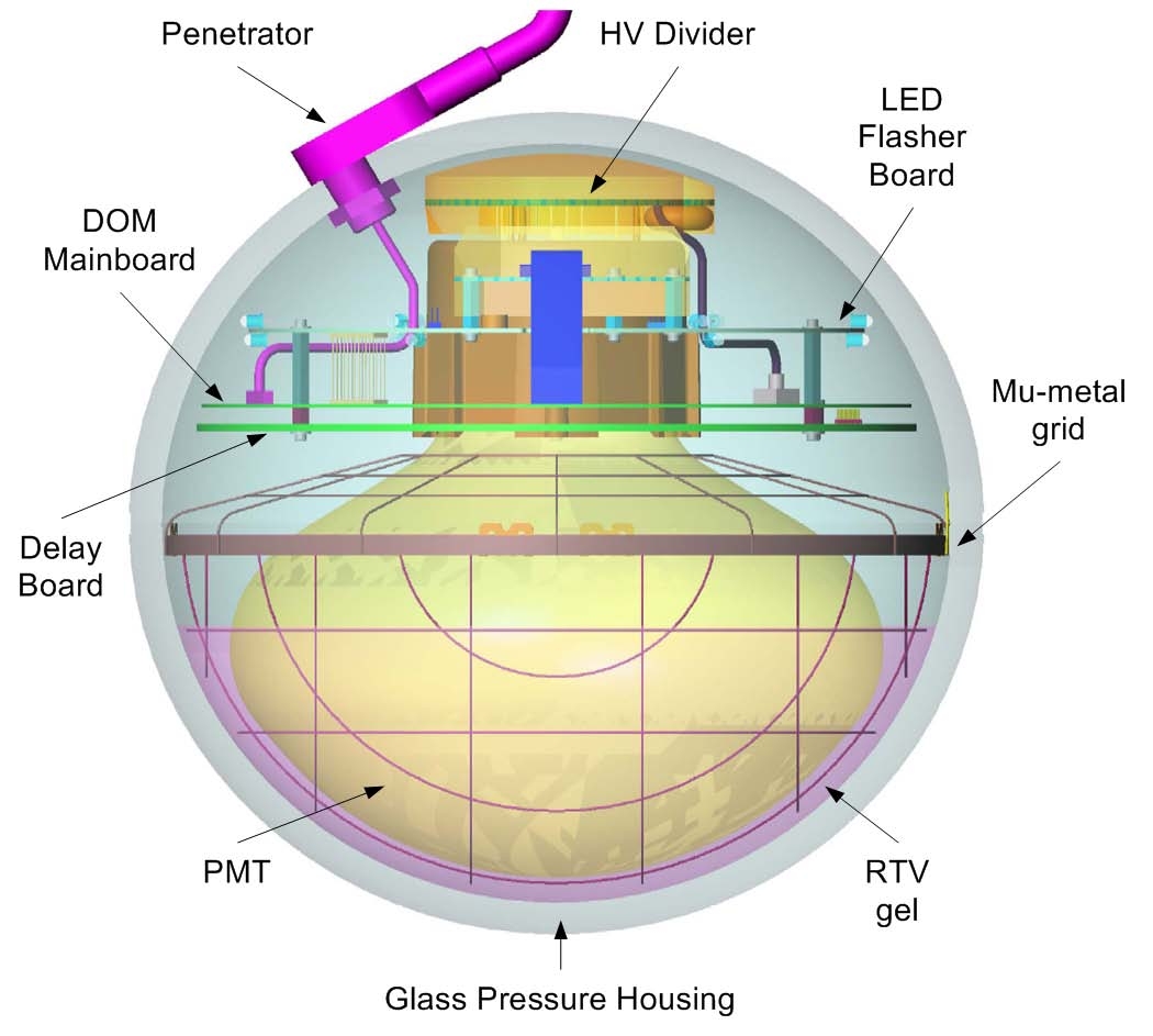
4.3.1 The Digital Optical Module . . . . . . . . . . . . . . . . . . . . . . . . . . . . . 59

4.3.2 IceCube DAQ . . . . . . . . . . . . . . . . . . . . . . . . . . . . . . . . . . . . . 60

4.3.2.1 Local Coincidence . . . . . . . . . . . . . . . . . . . . . . . . . . . . . 61

5 Gamma-Ray Burst Selection

5.1 Satellites . . . . . . . . . . . . . . . . . . . . . . . . . . . . . . . . . . . . . . . . . . . . 66

5.2 Blindness . . . . . . . . . . . . . . . . . . . . . . . . . . . . . . . . . . . . . . . . . . . 67

5.3 AMANDA-II . . . . . . . . . . . . . . . . . . . . . . . . . . . . . . . . . . . . . . . . . 67

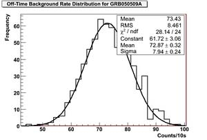
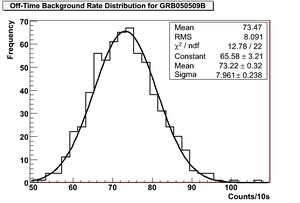
5.3.1 Detector Stability Criteria . . . . . . . . . . . . . . . . . . . . . . . . . . . . . . 68

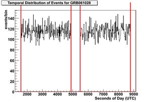
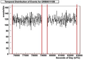
5.3.2 Burst Duration Determination . . . . . . . . . . . . . . . . . . . . . . . . . . . 70

5.4 IceCube . . . . . . . . . . . . . . . . . . . . . . . . . . . . . . . . . . . . . . . . . . . . 74

5.4.1 Detector Stability Criteria . . . . . . . . . . . . . . . . . . . . . . . . . . . . . . 75

5.4.2 Burst Duration Determination . . . . . . . . . . . . . . . . . . . . . . . . . . . 75

6 Simulation

6.1 Generators . . . . . . . . . . . . . . . . . . . . . . . . . . . . . . . . . . . . . . . . . . 78

6.2 Propagators . . . . . . . . . . . . . . . . . . . . . . . . . . . . . . . . . . . . . . . . . . 79

6.3 Detector Simulation . . . . . . . . . . . . . . . . . . . . . . . . . . . . . . . . . . . . . 79

6.3.1 AMANDA . . . . . . . . . . . . . . . . . . . . . . . . . . . . . . . . . . . . . . . 80

6.3.2 IceCube . . . . . . . . . . . . . . . . . . . . . . . . . . . . . . . . . . . . . . . . 80

7 AMANDA-II Analysis

7.1 Filtering . . . . . . . . . . . . . . . . . . . . . . . . . . . . . . . . . . . . . . . . . . . . 81

7.1.1 Level 1 Filter . . . . . . . . . . . . . . . . . . . . . . . . . . . . . . . . . . . . . 81

7.1.2 Level 2 Filter . . . . . . . . . . . . . . . . . . . . . . . . . . . . . . . . . . . . . 83

7.1.3 Level 3 Filter . . . . . . . . . . . . . . . . . . . . . . . . . . . . . . . . . . . . . 83

7.1.4 Flare Checking . . . . . . . . . . . . . . . . . . . . . . . . . . . . . . . . . . . . 83

7.1.5 Starting Dataset . . . . . . . . . . . . . . . . . . . . . . . . . . . . . . . . . . . 84

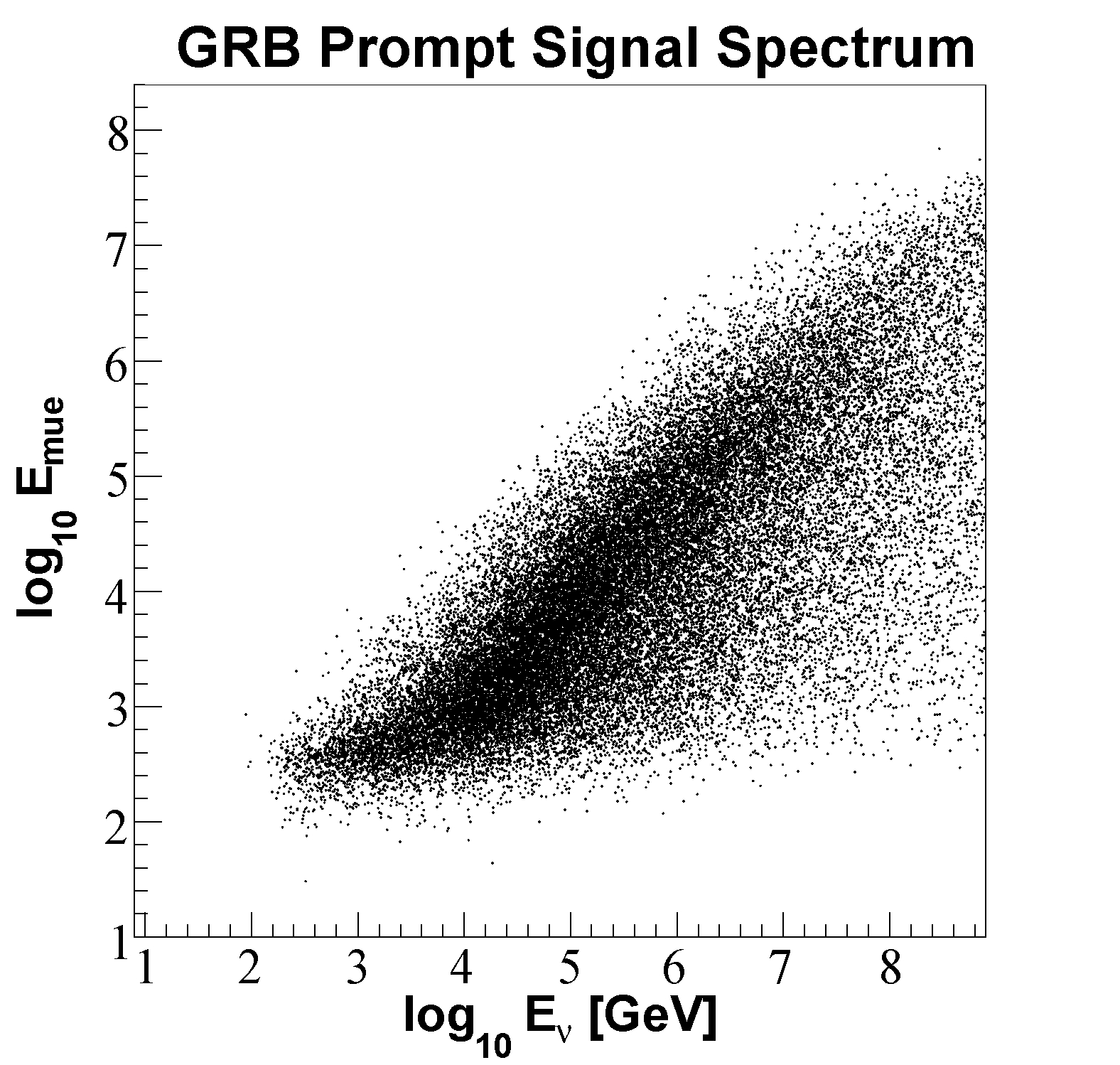
7.2 Signal Spectrum . . . . . . . . . . . . . . . . . . . . . . . . . . . . . . . . . . . . . . . 84

7.3 Event Selection Variables . . . . . . . . . . . . . . . . . . . . . . . . . . . . . . . . . . 86

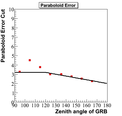
7.3.1 Paraboloid Sigma . . . . . . . . . . . . . . . . . . . . . . . . . . . . . . . . . . . 86

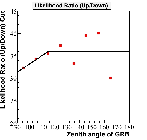
7.3.2 Likelihood Ratio . . . . . . . . . . . . . . . . . . . . . . . . . . . . . . . . . . . 87

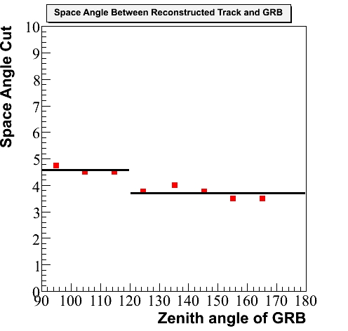
7.3.3 Space Angle . . . . . . . . . . . . . . . . . . . . . . . . . . . . . . . . . . . . . . 88

7.3.4 Other Variables . . . . . . . . . . . . . . . . . . . . . . . . . . . . . . . . . . . . 90

7.3.5 Temporal Coincidence . . . . . . . . . . . . . . . . . . . . . . . . . . . . . . . . 91

7.4 Optimization . . . . . . . . . . . . . . . . . . . . . . . . . . . . . . . . . . . . . . . . . 91

7.5 Final Event Sample . . . . . . . . . . . . . . . . . . . . . . . . . . . . . . . . . . . . . . 98

7.6 Sensitivity . . . . . . . . . . . . . . . . . . . . . . . . . . . . . . . . . . . . . . . . . . . 99

7.7 Discovery Potential . . . . . . . . . . . . . . . . . . . . . . . . . . . . . . . . . . . . . . 101

7.8 Results . . . . . . . . . . . . . . . . . . . . . . . . . . . . . . . . . . . . . . . . . . . . . 102

8 IceCube Analysis

107

8.1 Filtering . . . . . . . . . . . . . . . . . . . . . . . . . . . . . . . . . . . . . . . . . . . . 107

8.1.1 Online Muon Filter / Level 1 Filter . . . . . . . . . . . . . . . . . . . . . . . . 108

8.1.2 Level 2 Filter . . . . . . . . . . . . . . . . . . . . . . . . . . . . . . . . . . . . . 108

8.1.3 Level 3 Filter . . . . . . . . . . . . . . . . . . . . . . . . . . . . . . . . . . . . . 108

8.1.4 Starting Event Sample . . . . . . . . . . . . . . . . . . . . . . . . . . . . . . . . 109

8.2 Signal Spectrum . . . . . . . . . . . . . . . . . . . . . . . . . . . . . . . . . . . . . . . 109

8.2.1 Precursor Emission . . . . . . . . . . . . . . . . . . . . . . . . . . . . . . . . . . 109

8.2.2 Prompt Emission . . . . . . . . . . . . . . . . . . . . . . . . . . . . . . . . . . . 111

8.2.3 Extended Window Search . . . . . . . . . . . . . . . . . . . . . . . . . . . . . . 115

8.3 Event Selection . . . . . . . . . . . . . . . . . . . . . . . . . . . . . . . . . . . . . . . . 116

8.3.1 Reduced Log-Likelihood . . . . . . . . . . . . . . . . . . . . . . . . . . . . . . . 116

8.3.2 Bayesian Likelihood Ratio . . . . . . . . . . . . . . . . . . . . . . . . . . . . . . 117

8.3.3 Paraboloid Sigma . . . . . . . . . . . . . . . . . . . . . . . . . . . . . . . . . . . 117

8.3.4 Umbrella Likelihood Ratio . . . . . . . . . . . . . . . . . . . . . . . . . . . . . . 117

8.3.5 Split Reconstruction Minimum Zenith . . . . . . . . . . . . . . . . . . . . . . . 117

8.3.6 Direct Hits . . . . . . . . . . . . . . . . . . . . . . . . . . . . . . . . . . . . . . 118

8.3.7 Cut Selection and Neutrino Level Sample . . . . . . . . . . . . . . . . . . . . . 118

8.4 Unbinned Analysis Method . . . . . . . . . . . . . . . . . . . . . . . . . . . . . . . . . 124

8.5 Sensitivity and Discovery Potential . . . . . . . . . . . . . . . . . . . . . . . . . . . . . 131

8.5.1 Trials Factors . . . . . . . . . . . . . . . . . . . . . . . . . . . . . . . . . . . . . 132

8.6 Results . . . . . . . . . . . . . . . . . . . . . . . . . . . . . . . . . . . . . . . . . . . . . 134

9 Systematic Error Analysis

136

9.1 Sources of Systematic Error . . . . . . . . . . . . . . . . . . . . . . . . . . . . . . . . . 137

9.1.1 Neutrino Cross-Section . . . . . . . . . . . . . . . . . . . . . . . . . . . . . . . . 137

9.1.2 Muon Propagation / Earth Model . . . . . . . . . . . . . . . . . . . . . . . . . 137

9.1.3 Reconstruction Bias . . . . . . . . . . . . . . . . . . . . . . . . . . . . . . . . . 138

9.1.4 Ice Properties . . . . . . . . . . . . . . . . . . . . . . . . . . . . . . . . . . . . . 138

9.1.5 Timing Resolution . . . . . . . . . . . . . . . . . . . . . . . . . . . . . . . . . . 139

9.1.6 (D)OM Efficiency . . . . . . . . . . . . . . . . . . . . . . . . . . . . . . . . . . 140

9.1.7 Seasonal Background Variations . . . . . . . . . . . . . . . . . . . . . . . . . . 140

10 Conclusions

142

10.1 Summary . . . . . . . . . . . . . . . . . . . . . . . . . . . . . . . . . . . . . . . . . . . 142

10.2 Discussion . . . . . . . . . . . . . . . . . . . . . . . . . . . . . . . . . . . . . . . . . . . 143

10.2.1 Previous Results . . . . . . . . . . . . . . . . . . . . . . . . . . . . . . . . . . . 143

10.2.2 Sensitivity to gamma rays from GRBs . . . . . . . . . . . . . . . . . . . . . . . 147

10.3 Outlook . . . . . . . . . . . . . . . . . . . . . . . . . . . . . . . . . . . . . . . . . . . . 149

Bibliography

152

A List of Abbreviations

160

B Sensitivity Studies for the Full Detector

163

B.1 Geometries . . . . . . . . . . . . . . . . . . . . . . . . . . . . . . . . . . . . . . . . . . 163

B.2 GRB Sample . . . . . . . . . . . . . . . . . . . . . . . . . . . . . . . . . . . . . . . . . 163

B.3 Event Selection . . . . . . . . . . . . . . . . . . . . . . . . . . . . . . . . . . . . . . . . 164

vii

B.4 Method . . . . . . . . . . . . . . . . . . . . . . . . . . . . . . . . . . . . . . . . . . . . 166

C Event Selection with Support Vector Machines

170

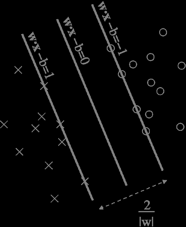
C.1 Fully Separable, Linear Case . . . . . . . . . . . . . . . . . . . . . . . . . . . . . . . . 171

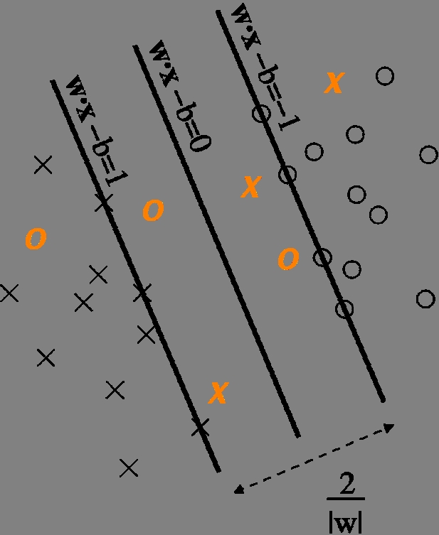
C.2 Non-Separable, Linear Case (Soft Margin) . . . . . . . . . . . . . . . . . . . . . . . . . 173

C.3 Non-Linear Case . . . . . . . . . . . . . . . . . . . . . . . . . . . . . . . . . . . . . . . 175

C.4 Example Application to a GRB Analysis . . . . . . . . . . . . . . . . . . . . . . . . . . 176

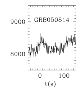
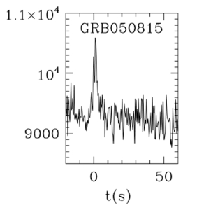
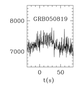
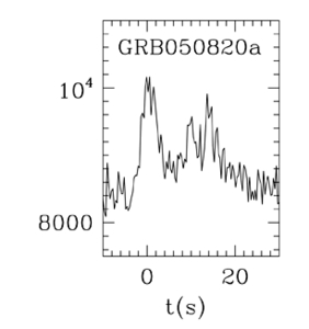
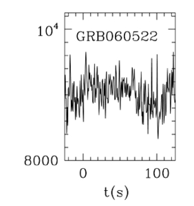
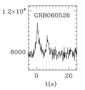
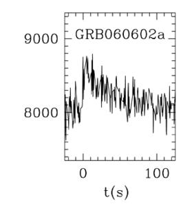
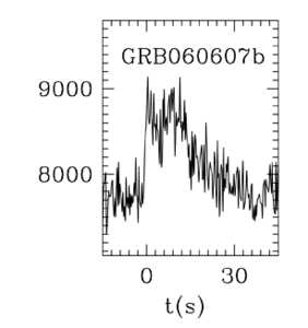
D Light Curves of 2005-2006 Northern Sky GRBs

184

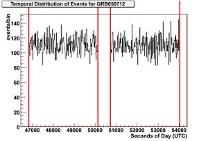
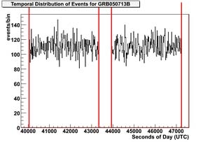
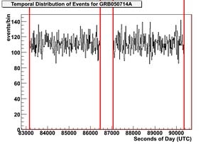
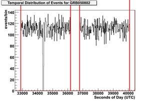
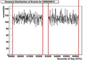
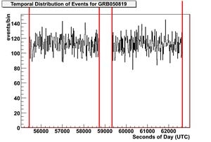
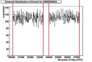
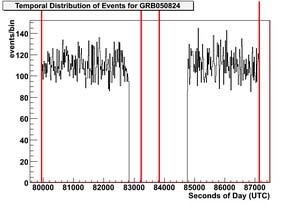
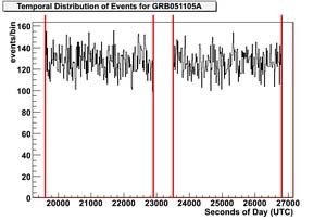
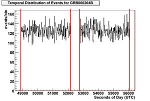
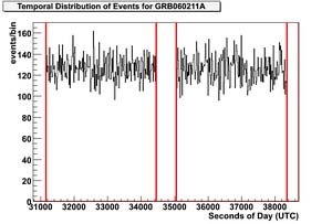
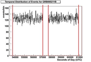
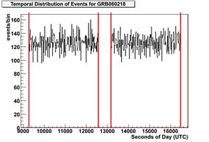
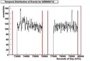
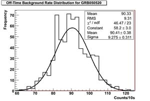
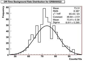
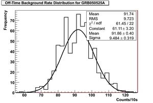
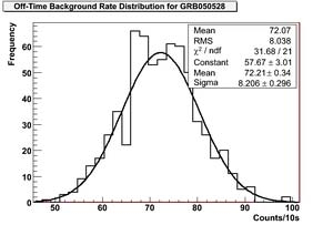
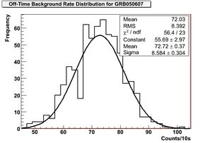
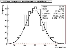
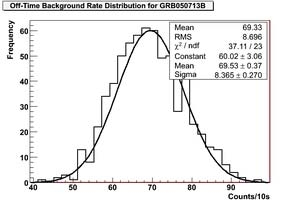
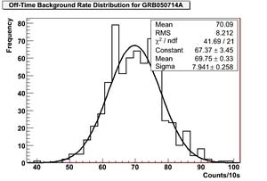
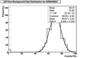
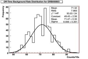
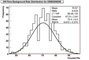
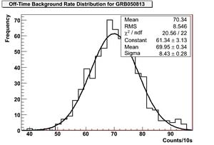
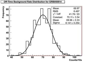
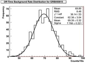
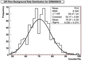
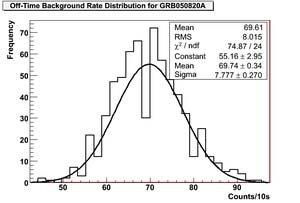
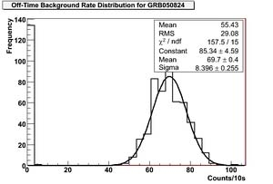
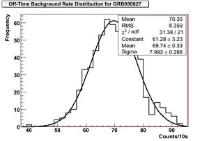
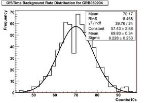
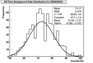
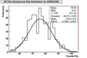
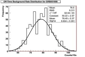
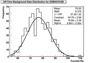
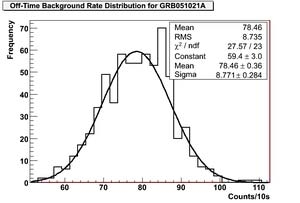
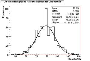
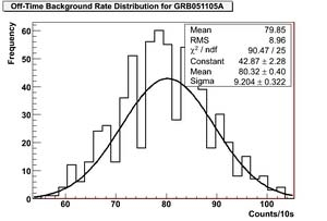
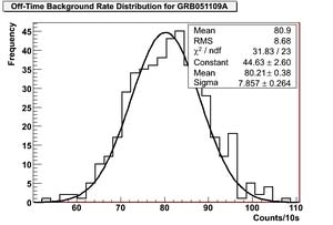
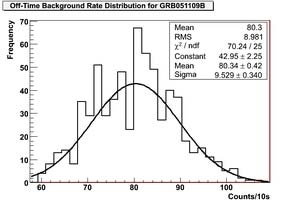
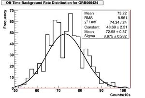
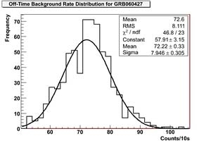
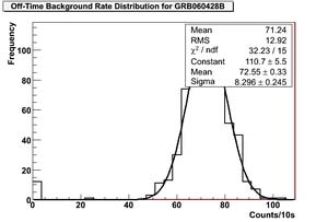
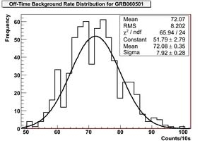
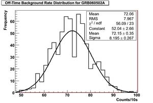
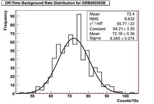
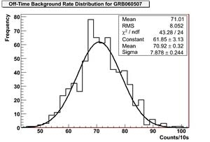
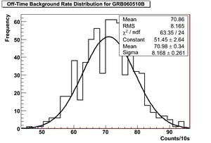
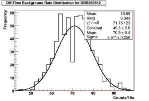
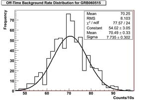
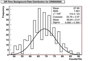
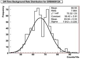
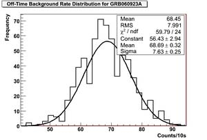
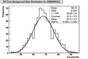
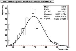
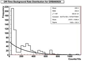
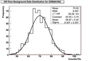
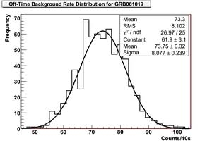
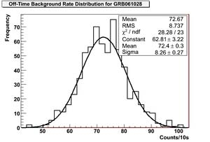
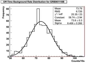
E Stability Plots for 2005-2006 Northern Sky GRBs

187

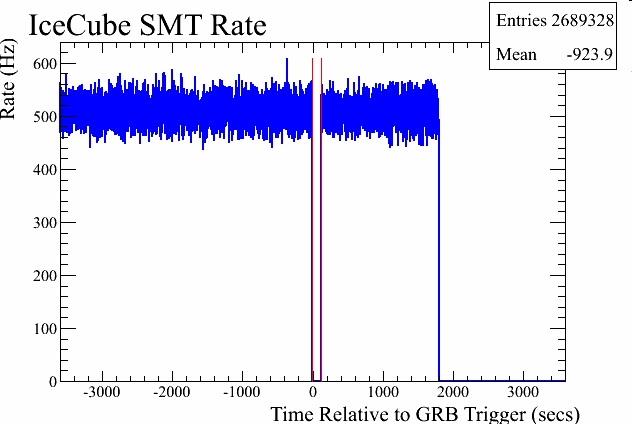
E.1 Filter Level Rates in Background Windows . . . . . . . . . . . . . . . . . . . . . . . . 187

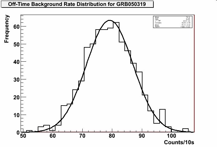
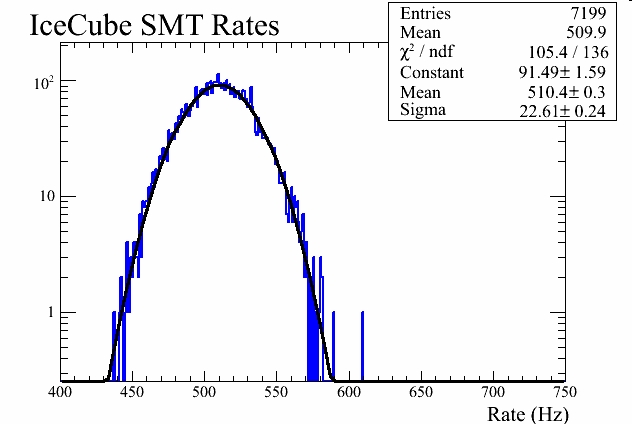
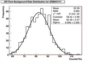
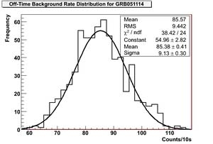
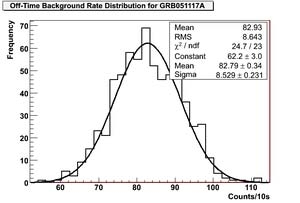
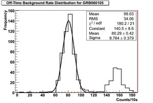
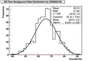
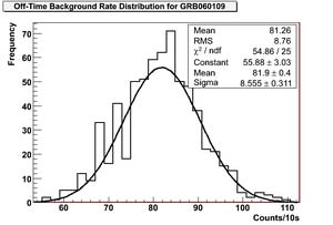
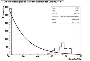
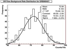
E.2 Distribution in Filter Level Rate per 10s . . . . . . . . . . . . . . . . . . . . . . . . . . 192

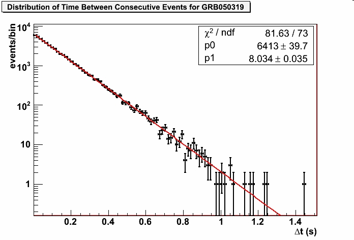
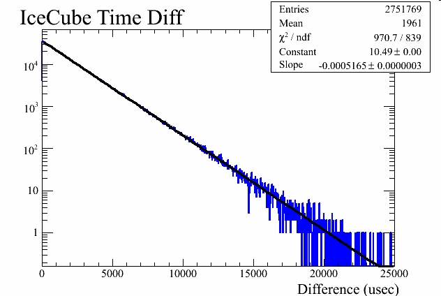
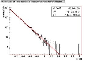
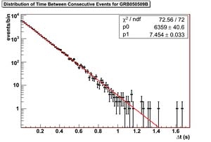
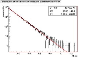
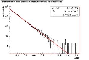
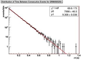
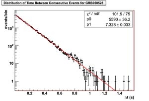
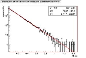
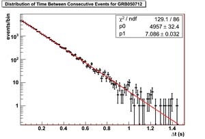
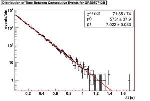
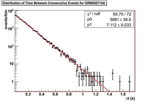
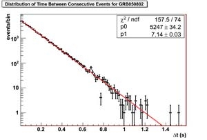
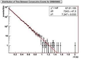
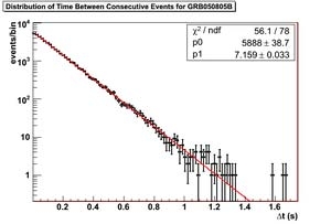
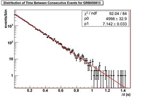
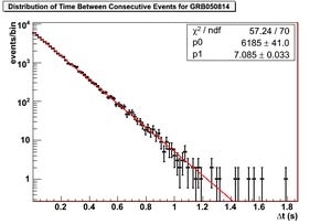
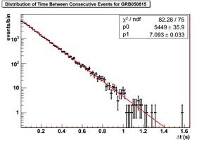
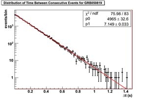
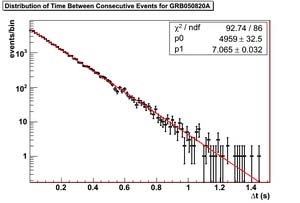
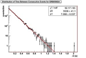
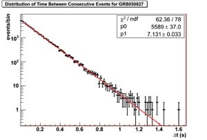
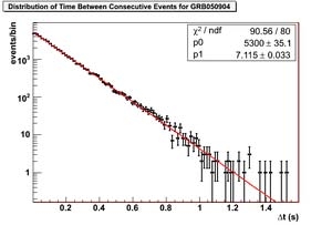
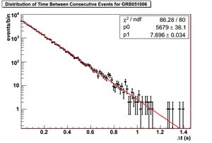
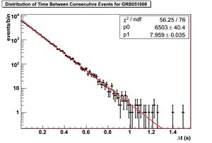
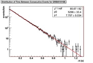
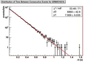
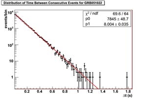
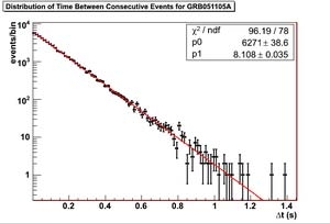
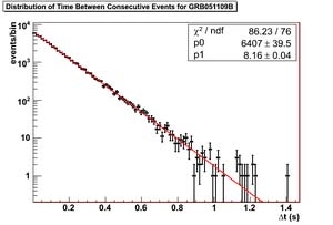
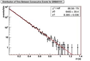
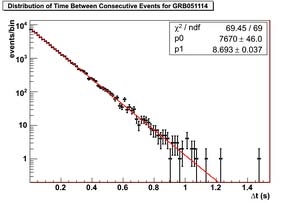
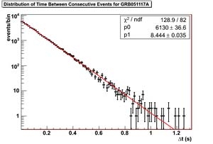
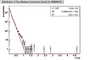
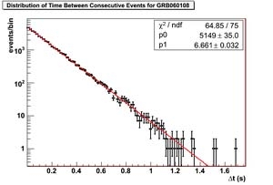
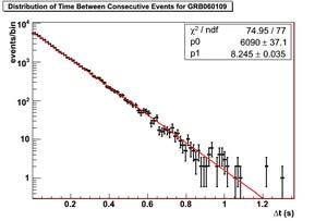
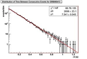
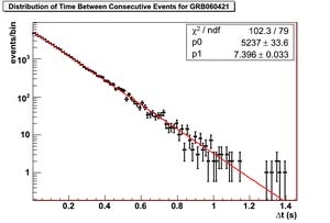
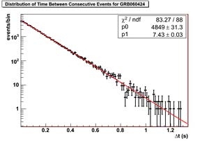
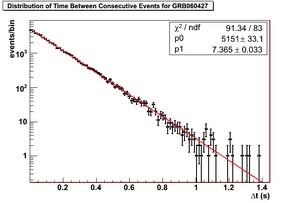
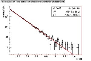
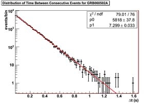
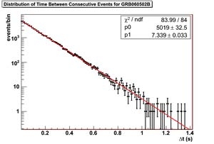
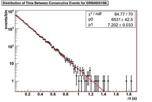
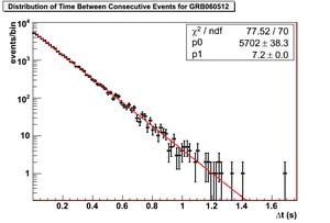
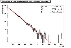
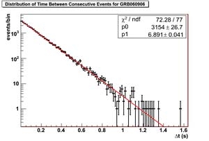
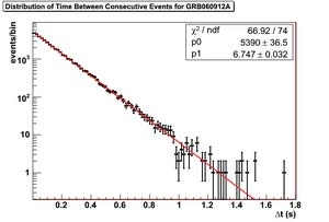
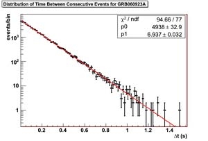
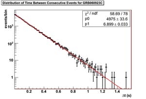
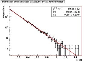
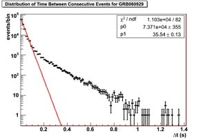
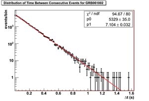
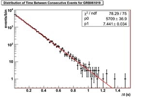
E.3 Time Differences Between Subsequent Events . . . . . . . . . . . . . . . . . . . . . . . 197

viii

List of Tables

2.1 Average BATSE GRB Parameters . . . . . . . . . . . . . . . . . . . . . . . . . . . . . 29

4.1 Main Parameters of GRB-detecting Satellites . . . . . . . . . . . . . . . . . . . . . . . 53

5.1 GRBs Lacking Detector Data in 2005-2006 . . . . . . . . . . . . . . . . . . . . . . . . 68

5.2 GRBs with Incomplete Stability Windows in 2005-2006 . . . . . . . . . . . . . . . . . 69

5.3 GRBs with Problem Data in 2005-2006 . . . . . . . . . . . . . . . . . . . . . . . . . . 71

5.4 2005-2006 Burst Sample . . . . . . . . . . . . . . . . . . . . . . . . . . . . . . . . . . . 72

5.5 GRBs with Problem Data in 2007-2008 . . . . . . . . . . . . . . . . . . . . . . . . . . 76

5.6 2007-2008 Burst Sample . . . . . . . . . . . . . . . . . . . . . . . . . . . . . . . . . . . 77

7.1 Summary of 2005-2006 AMANDA-II upgoing muon filters. . . . . . . . . . . . . . . . . 82

7.2 AMANDA-II upgoing filter passing rates. . . . . . . . . . . . . . . . . . . . . . . . . . 84

7.3 Event Selection for the 2005-2006 AMANDA analysis . . . . . . . . . . . . . . . . . . 94

7.4 Final Event Rates for 2005-2006 . . . . . . . . . . . . . . . . . . . . . . . . . . . . . . 98

7.5 Discovery Potential for 2005-2006 . . . . . . . . . . . . . . . . . . . . . . . . . . . . . . 104

8.1 Summary of 22-string IceCube upgoing muon filters. . . . . . . . . . . . . . . . . . . . 108

8.2 Average Parameters for Swift GRBs . . . . . . . . . . . . . . . . . . . . . . . . . . . . 112

8.3 GRB Spectral Information for 2007-2008 . . . . . . . . . . . . . . . . . . . . . . . . . . 113

8.4 Modified Extended Time Windows . . . . . . . . . . . . . . . . . . . . . . . . . . . . . 116

8.5 Event Selection Criteria for 2007-2008 . . . . . . . . . . . . . . . . . . . . . . . . . . . 119

8.6 Final Event Rates for 2007-2008 . . . . . . . . . . . . . . . . . . . . . . . . . . . . . . 121

8.7 Sensitivity and Discovery Potential for 2007-2008 . . . . . . . . . . . . . . . . . . . . . 133

8.8 Upper Limits for 2007-2008 . . . . . . . . . . . . . . . . . . . . . . . . . . . . . . . . . 135

9.1 AMANDA-II Systematic Errors . . . . . . . . . . . . . . . . . . . . . . . . . . . . . . . 136

9.2 IceCube Systematic Errors . . . . . . . . . . . . . . . . . . . . . . . . . . . . . . . . . . 137

10.1 Results of Previous and Current GRB Searches . . . . . . . . . . . . . . . . . . . . . . 143

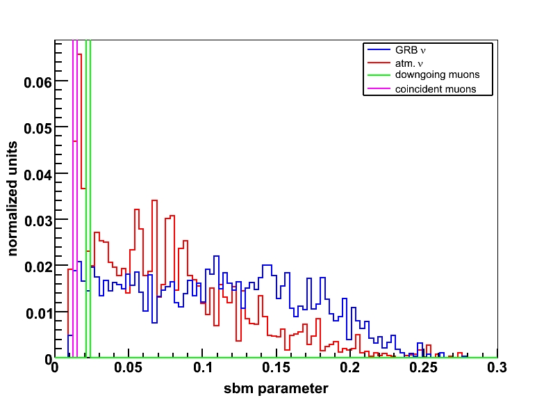
B.1 Simulation Remaining After SBM Selection . . . . . . . . . . . . . . . . . . . . . . . . 165

B.2 Event Rates for the Full IceCube Detector . . . . . . . . . . . . . . . . . . . . . . . . . 168

List of Figures

1.1 The Cosmic Ray Spectrum . . . . . . . . . . . . . . . . . . . . . . . . . . . . . . . . .

1.2 First Order Fermi Acceleration . . . . . . . . . . . . . . . . . . . . . . . . . . . . . . .

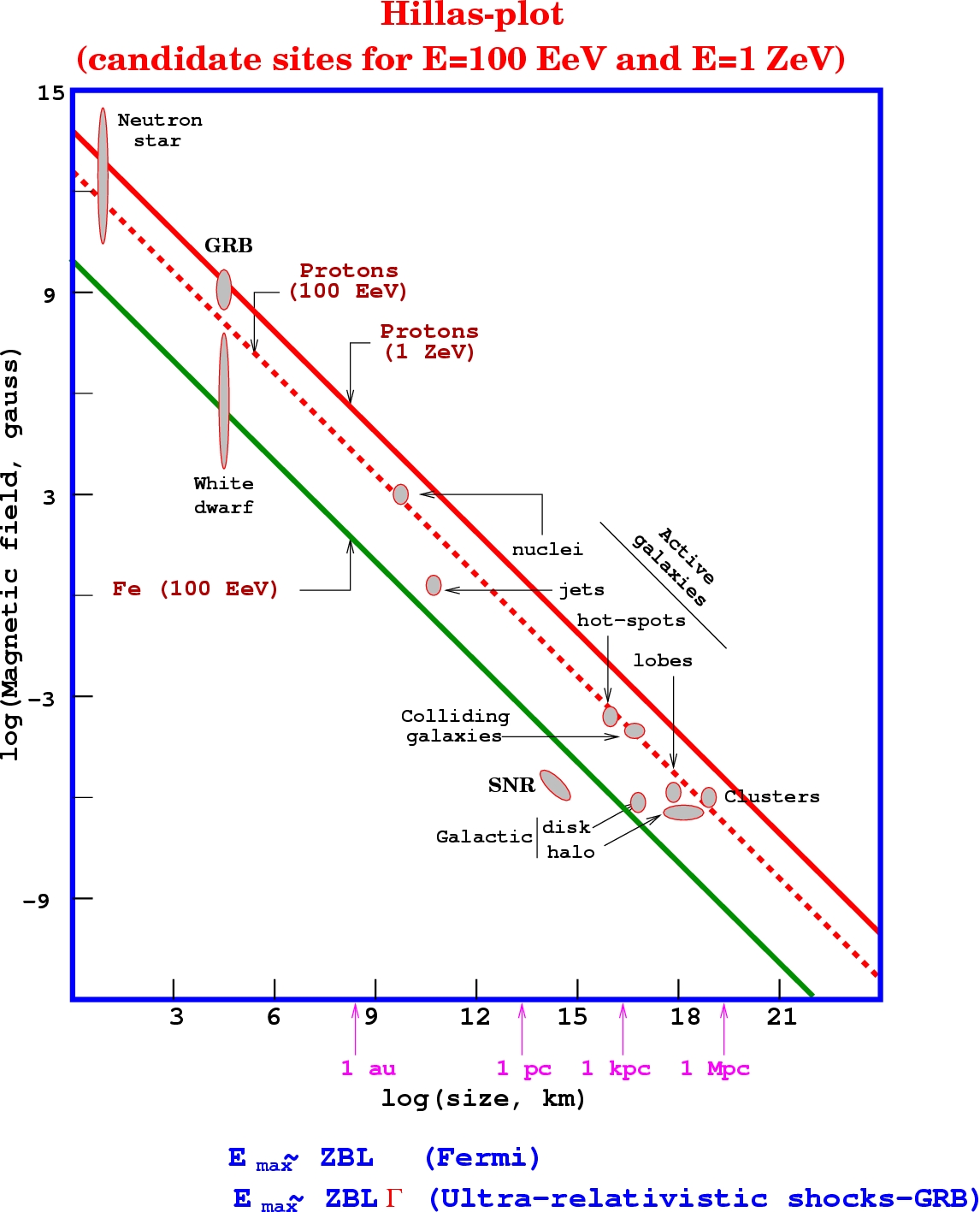
1.3 Hillas Diagram . . . . . . . . . . . . . . . . . . . . . . . . . . . . . . . . . . . . . . . .

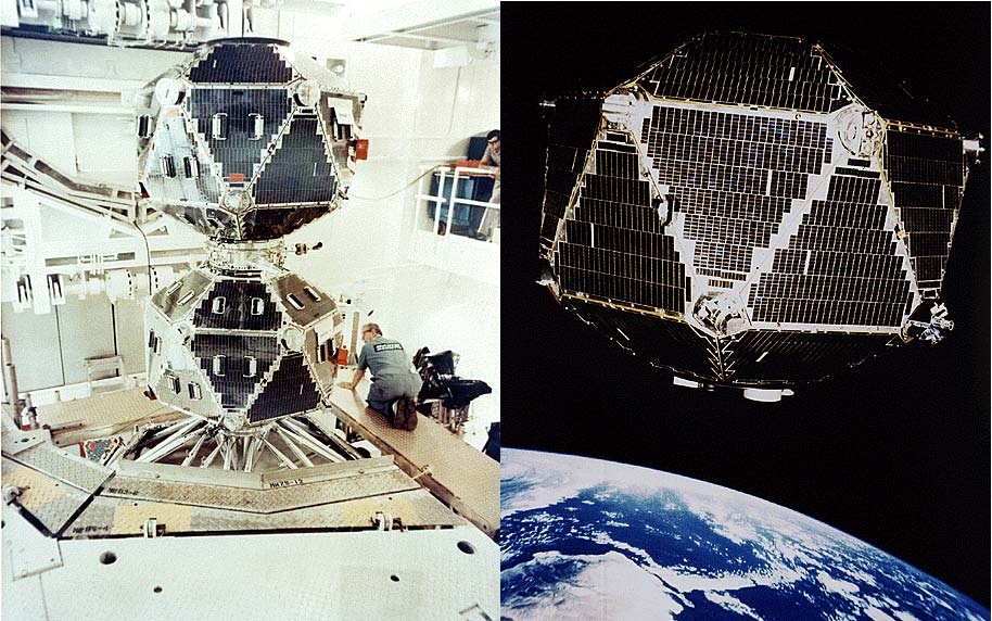
2.1 The Vela 5 Satellite . . . . . . . . . . . . . . . . . . . . . . . . . . . . . . . . . . . . . 13

2.2 GRB Duration Distribution . . . . . . . . . . . . . . . . . . . . . . . . . . . . . . . . . 14

2.3 GRB Spatial Distribution . . . . . . . . . . . . . . . . . . . . . . . . . . . . . . . . . . 15

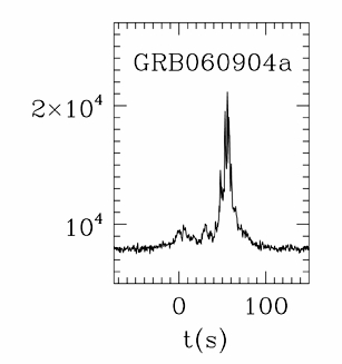
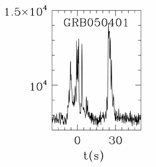
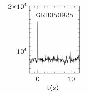
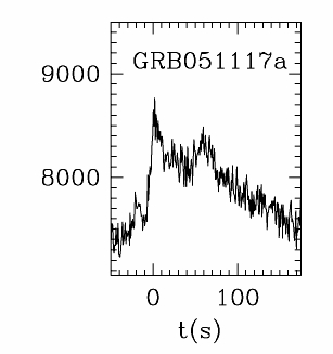
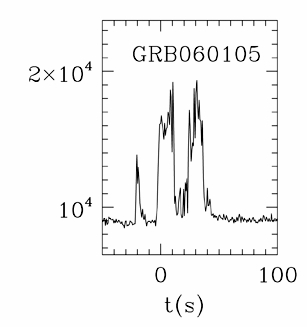
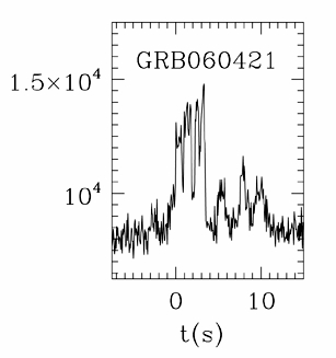
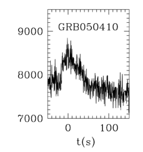
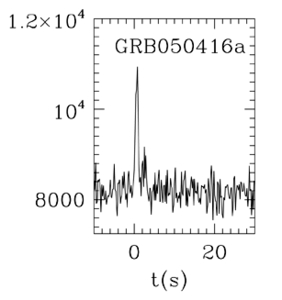
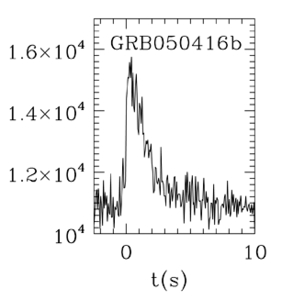
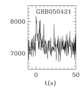
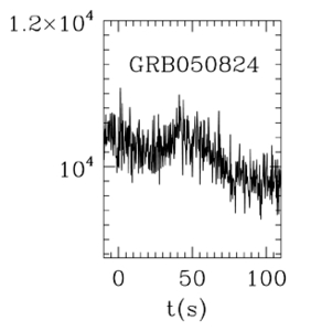
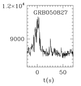
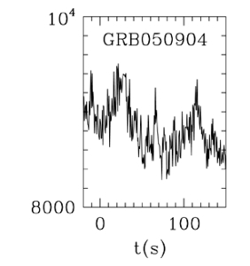
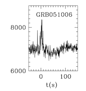
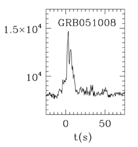
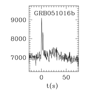
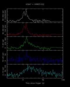
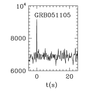
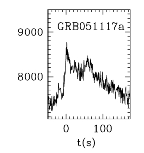
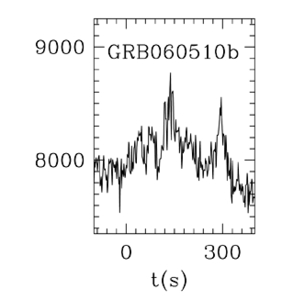
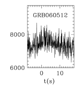
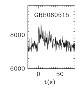
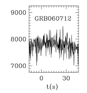
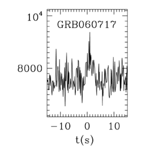
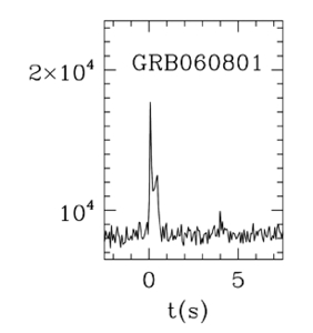
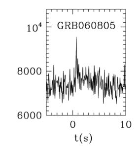
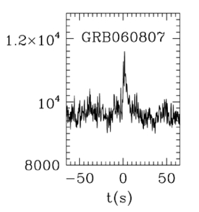
2.4 Sample GRB Lightcurves . . . . . . . . . . . . . . . . . . . . . . . . . . . . . . . . . . 17

2.5 Effect of Relativistic Aberration on Time Variability . . . . . . . . . . . . . . . . . . . 19

2.6 Temporal Jet Break in GRB990510 . . . . . . . . . . . . . . . . . . . . . . . . . . . . . 22

2.7 Calibrated GRB Energy . . . . . . . . . . . . . . . . . . . . . . . . . . . . . . . . . . . 23

2.8 Prompt and Precursor Neutrino Emission in the Fireball Model . . . . . . . . . . . . . 28

3.1 Neutrino Cross-section and Interaction Length . . . . . . . . . . . . . . . . . . . . . . 34

3.2 Ceˇ renkov Radiation . . . . . . . . . . . . . . . . . . . . . . . . . . . . . . . . . . . . . 35

3.3 Muon Energy Loss in Ice . . . . . . . . . . . . . . . . . . . . . . . . . . . . . . . . . . . 37

3.4 Angular Distribution of Atmospheric Muons . . . . . . . . . . . . . . . . . . . . . . . . 39

3.5 The Earth as a Muon Filter . . . . . . . . . . . . . . . . . . . . . . . . . . . . . . . . . 39

3.6 Optical Properties of South Pole Ice . . . . . . . . . . . . . . . . . . . . . . . . . . . . 41

3.7 Reconstruction Parameters . . . . . . . . . . . . . . . . . . . . . . . . . . . . . . . . . 42

3.8 Pandel Parameterization of Light Delay . . . . . . . . . . . . . . . . . . . . . . . . . . 46

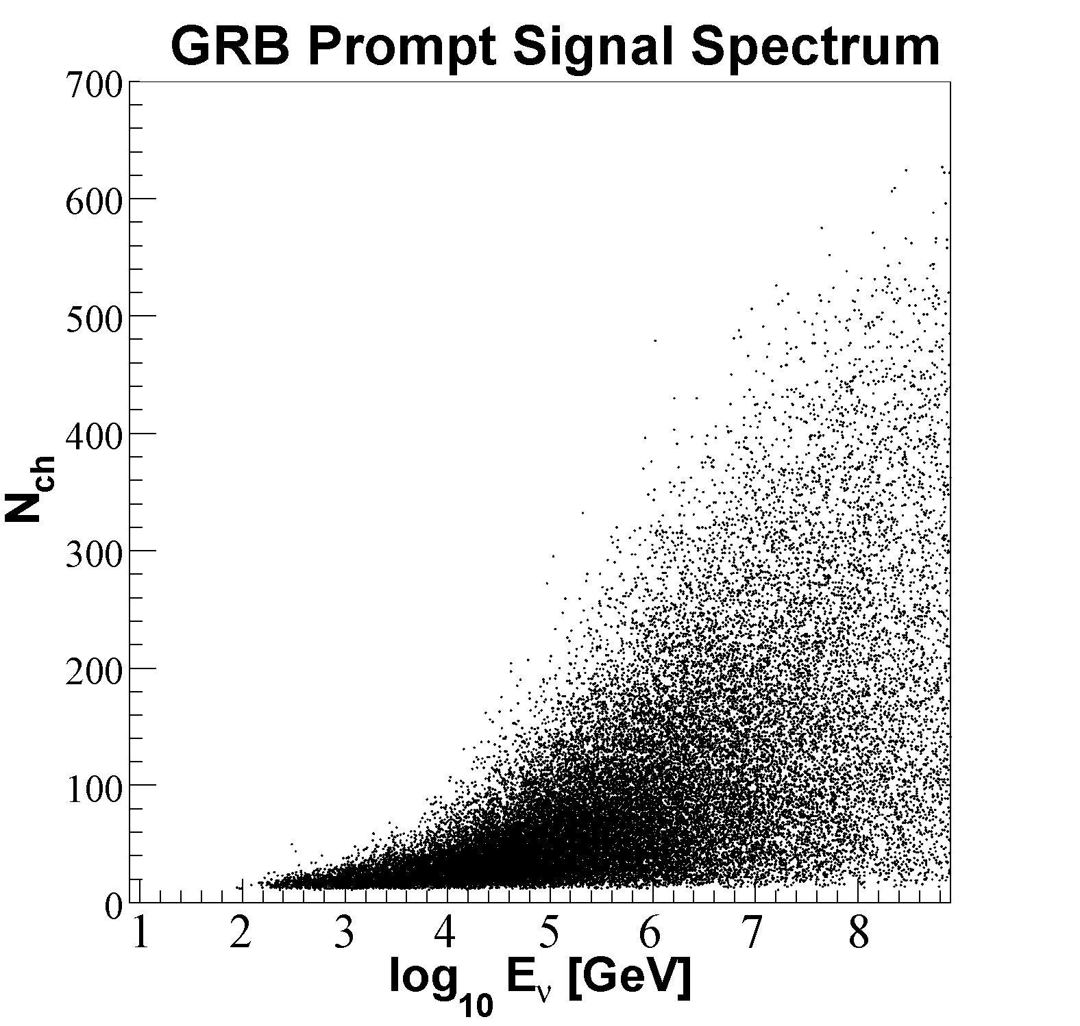
3.9 N

as a Function of Neutrino Energy . . . . . . . . . . . . . . . . . . . . . . . . . . . 49

3.10 N

Distribution for Various Spectra . . . . . . . . . . . . . . . . . . . . . . . . . . . . 50

3.11 ?

mue

as a Function of Neutrino Energy . . . . . . . . . . . . . . . . . . . . . . . . . . . 51

3.12 ?

mue

Distribution for Various Spectra . . . . . . . . . . . . . . . . . . . . . . . . . . . 51

3.13 Comparison of Energy Estimators . . . . . . . . . . . . . . . . . . . . . . . . . . . . . 52

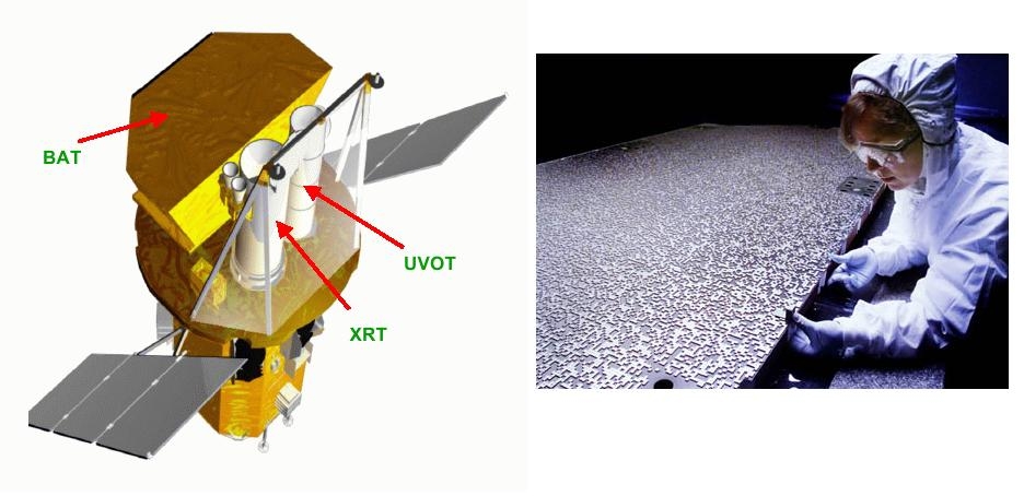
4.1 The Swift Satellite . . . . . . . . . . . . . . . . . . . . . . . . . . . . . . . . . . . . . . 54

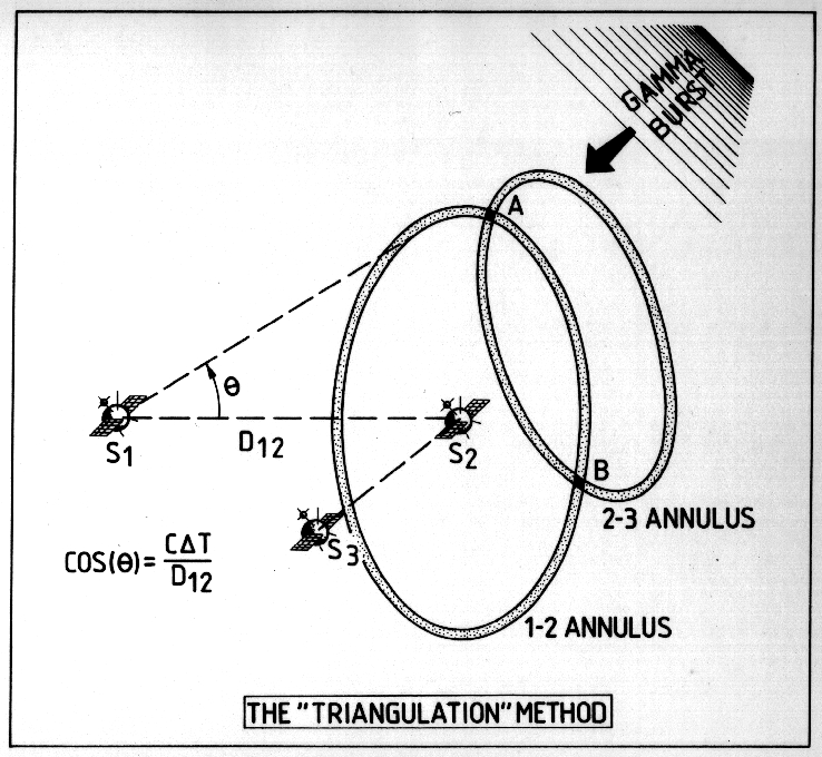
4.2 Triangulation with IPN3 . . . . . . . . . . . . . . . . . . . . . . . . . . . . . . . . . . . 56

4.3 The AMANDA-II Detector . . . . . . . . . . . . . . . . . . . . . . . . . . . . . . . . . 58

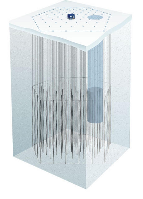
4.4 The IceCube Detector . . . . . . . . . . . . . . . . . . . . . . . . . . . . . . . . . . . . 62

4.5 Wavelength Dependence of DOM properties . . . . . . . . . . . . . . . . . . . . . . . . 63

4.6 Schematic of a DOM . . . . . . . . . . . . . . . . . . . . . . . . . . . . . . . . . . . . . 64

4.7 Sample ATWD and PMT ADC Waveforms . . . . . . . . . . . . . . . . . . . . . . . . 65

5.1 Blindness for GRB Searches . . . . . . . . . . . . . . . . . . . . . . . . . . . . . . . . . 67

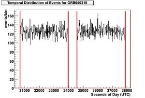
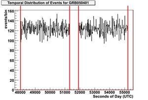
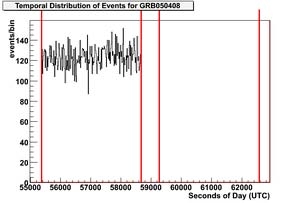
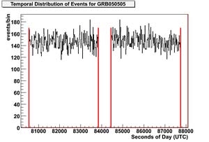
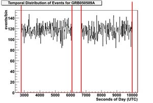
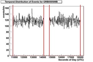
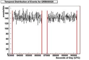
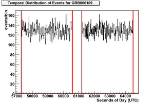
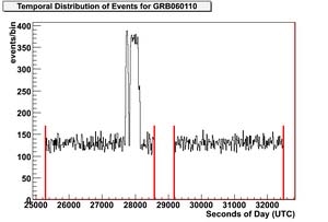
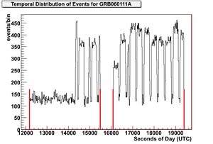
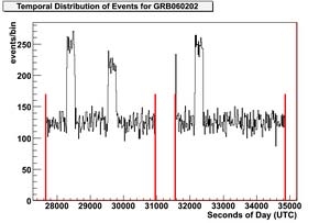
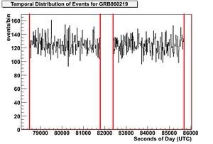
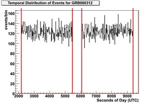
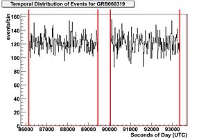
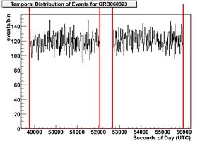
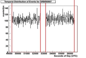
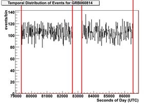
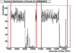
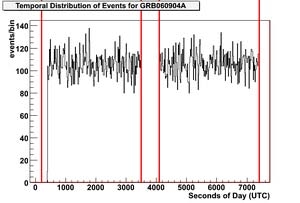
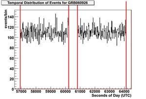
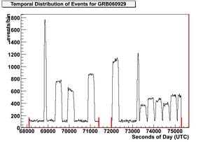
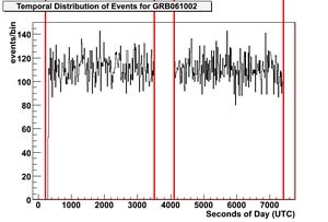
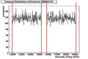
5.2 Sample AMANDA Stability Plots . . . . . . . . . . . . . . . . . . . . . . . . . . . . . . 70

5.3 Burst Duration Definition for 2005-2006 . . . . . . . . . . . . . . . . . . . . . . . . . . 72

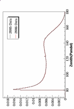
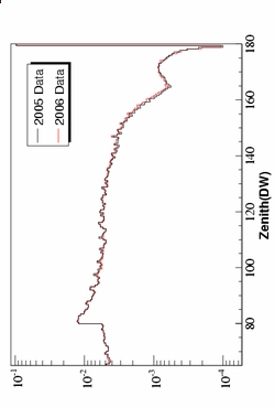
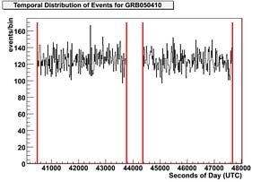
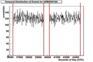
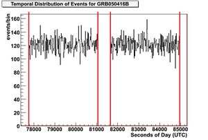
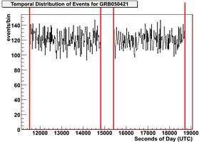
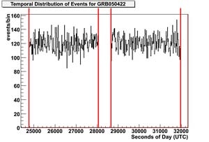
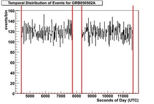
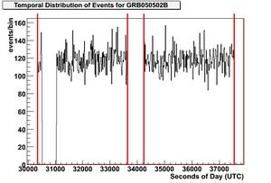
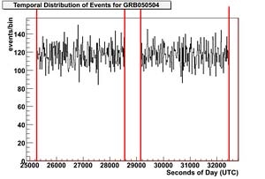
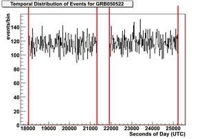
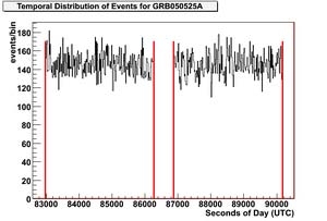
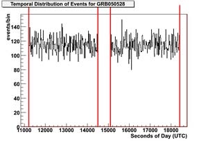
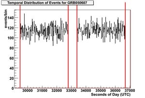
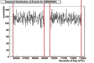
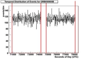
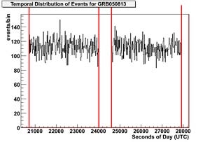
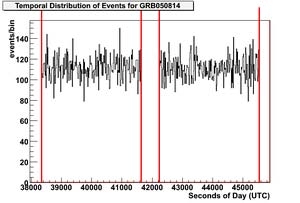
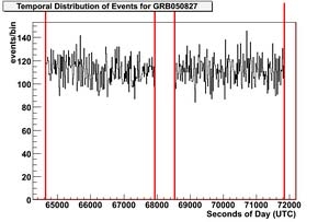
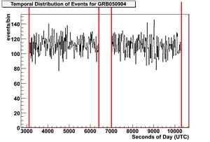
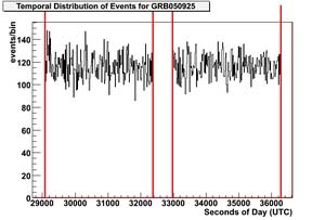
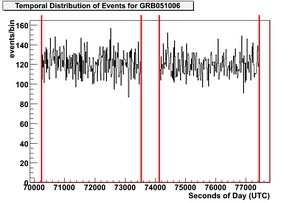
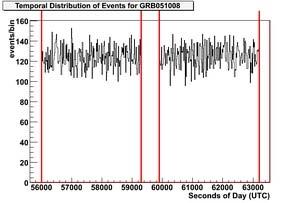
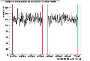
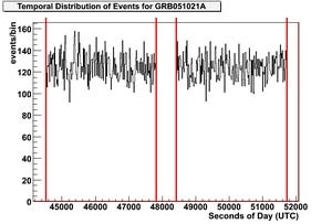
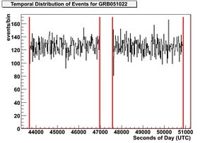
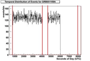
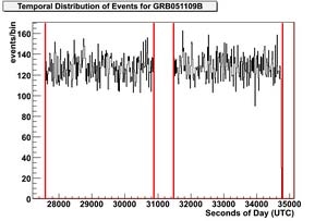
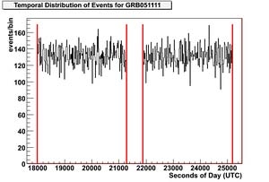
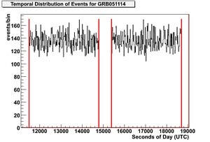
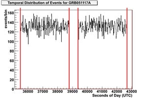
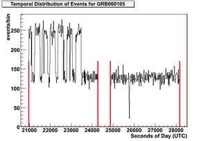
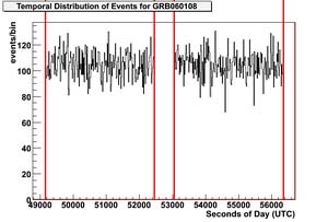
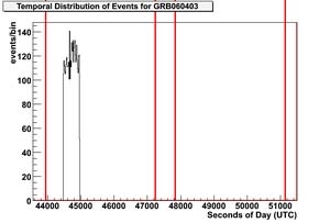
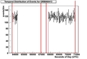
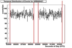
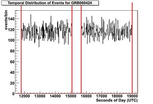
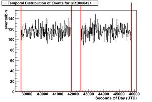
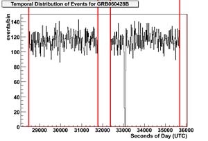
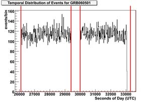
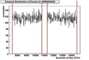
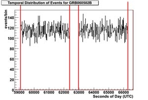
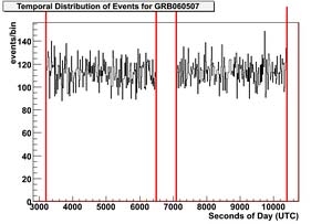
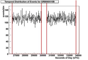
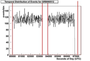
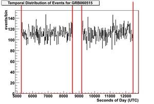
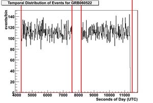
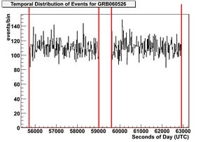
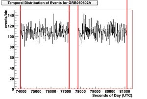
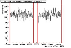
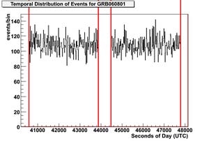
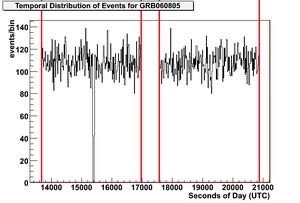
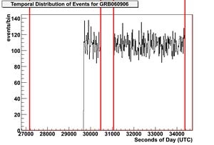
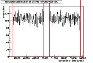
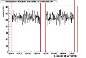
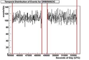
5.4 Sample IceCube Stability Plots . . . . . . . . . . . . . . . . . . . . . . . . . . . . . . . 76

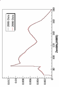
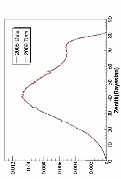
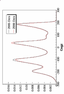
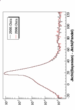
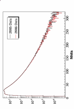
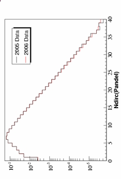
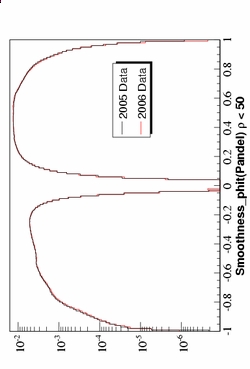
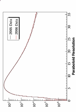
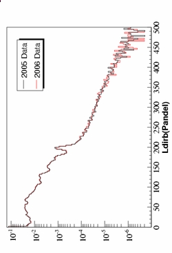
7.1 Comparison of 2005 and 2006 data . . . . . . . . . . . . . . . . . . . . . . . . . . . . . 85

7.2 AMANDA Response to GRB Signal at Filter Level . . . . . . . . . . . . . . . . . . . . 86

7.3 Background Contamination at Filter Level for 2005-2006 . . . . . . . . . . . . . . . . . 87

7.4 Paraboloid Sigma at Filter Level for 2005-2006 . . . . . . . . . . . . . . . . . . . . . . 88

7.5 Likelihood Ratio at Filter Level for 2005-2006 . . . . . . . . . . . . . . . . . . . . . . . 89

7.6 Space Angle at Filter Level for 2005-2006 . . . . . . . . . . . . . . . . . . . . . . . . . 89

7.7 Direct Hits Problem . . . . . . . . . . . . . . . . . . . . . . . . . . . . . . . . . . . . . 90

7.8 Cut Parameterization for 2005-2006 . . . . . . . . . . . . . . . . . . . . . . . . . . . . 95

7.9 Zenith Dependence of Parameter Distributions for 2005-2006 . . . . . . . . . . . . . . 96

7.10 Partial Cut Application for 2005-2006 . . . . . . . . . . . . . . . . . . . . . . . . . . . 97

7.11 Simulation and data comparison at final cut level for 2005-2006 . . . . . . . . . . . . . 99

7.12 Paraboloid Sigma at Final Cut Level for 2005-2006 . . . . . . . . . . . . . . . . . . . . 100

xii

7.13 Likelihood Ratio at Final Cut Level for 2005-2006 . . . . . . . . . . . . . . . . . . . . 101

7.14 Space Angle at Final Cut Level for 2005-2006 . . . . . . . . . . . . . . . . . . . . . . . 102

7.15 Final Cut Efficiency for 2005-2006 . . . . . . . . . . . . . . . . . . . . . . . . . . . . . 103

7.16 AMANDA Neutrino Effective Area . . . . . . . . . . . . . . . . . . . . . . . . . . . . . 104

7.17 Model Discovery Potential for 2005-2006 . . . . . . . . . . . . . . . . . . . . . . . . . . 105

7.18 Upper Limit of the AMANDA analysis . . . . . . . . . . . . . . . . . . . . . . . . . . . 106

8.1 Event Rates at Filter Level for 2007-2008 . . . . . . . . . . . . . . . . . . . . . . . . . 110

8.2 IceCube Response to Precursor Neutrinos . . . . . . . . . . . . . . . . . . . . . . . . . 111

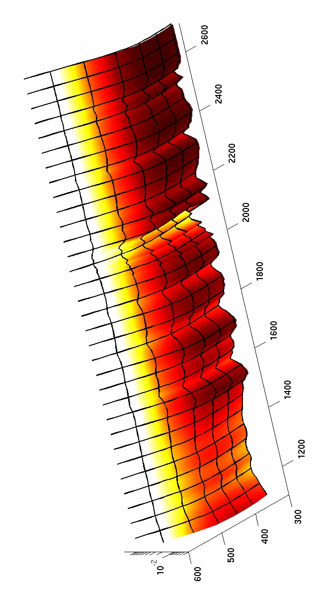
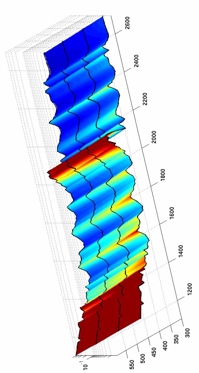
8.3 Neutrino Spectra for 41 GRBs Observed in 2007-2008 . . . . . . . . . . . . . . . . . . 115

8.4 Cut Efficiency for Several Event Selection Parameters . . . . . . . . . . . . . . . . . . 119

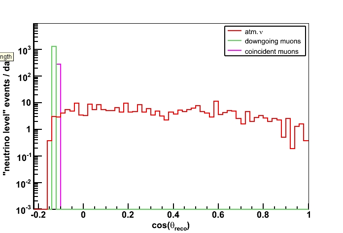
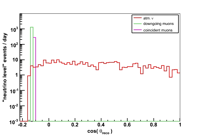
8.5 Event Rates at Neutrino Level for 2007-2008 . . . . . . . . . . . . . . . . . . . . . . . 120

8.6 Cumulative Point Spread Function for 2007-2008 . . . . . . . . . . . . . . . . . . . . . 121

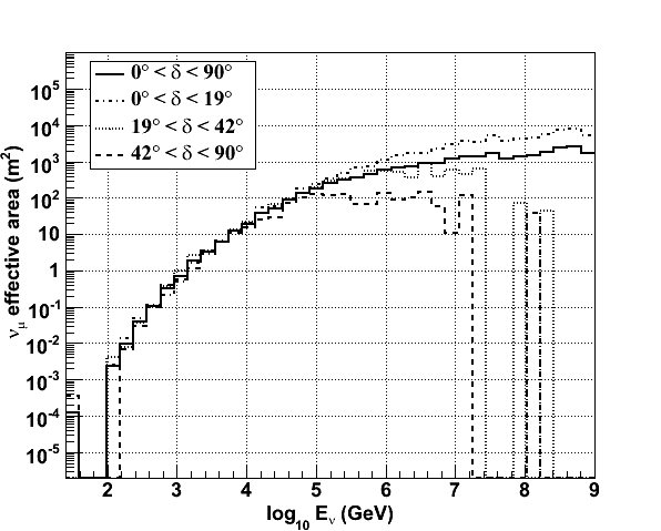
8.7 22-String IceCube Muon Neutrino Effective Area . . . . . . . . . . . . . . . . . . . . . 122

8.8 Signal Efficiency for 2007-2008 . . . . . . . . . . . . . . . . . . . . . . . . . . . . . . . 123

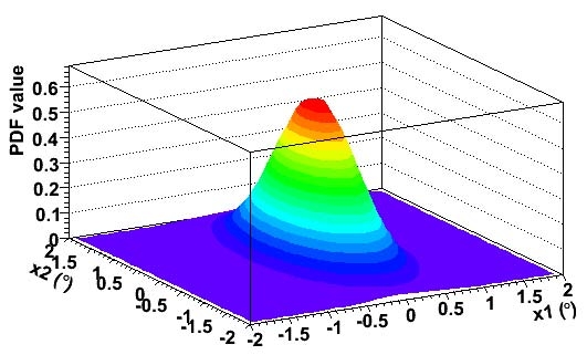
8.9 Spatial Signal PDF . . . . . . . . . . . . . . . . . . . . . . . . . . . . . . . . . . . . . . 127

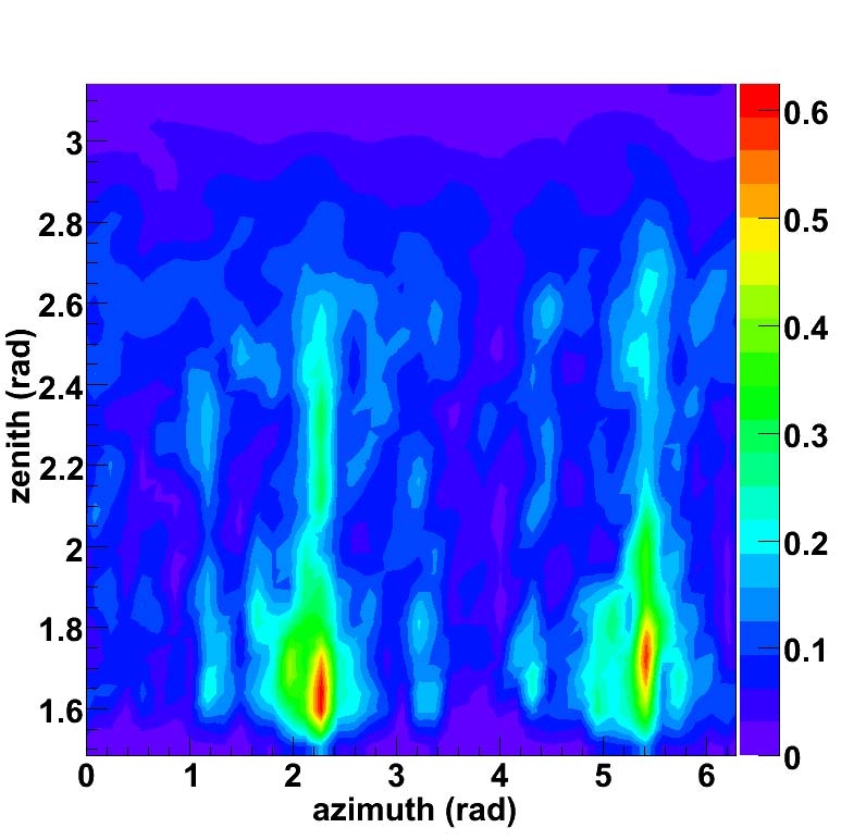
8.10 Spatial Background PDF for IceCube . . . . . . . . . . . . . . . . . . . . . . . . . . . 128

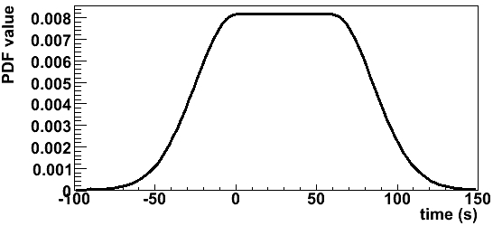
8.11 Temporal Signal PDF . . . . . . . . . . . . . . . . . . . . . . . . . . . . . . . . . . . . 128

8.12 Energy PDFs for Several Spectra . . . . . . . . . . . . . . . . . . . . . . . . . . . . . . 130

8.13 Test Statistic Distribution for Background Only Hypothesis . . . . . . . . . . . . . . . 131

8.14 Discovery Potential for 2007-2008 IceCube Analysis . . . . . . . . . . . . . . . . . . . . 133

8.15 Upper Limits for 2007-2008 IceCube Analysis . . . . . . . . . . . . . . . . . . . . . . . 135

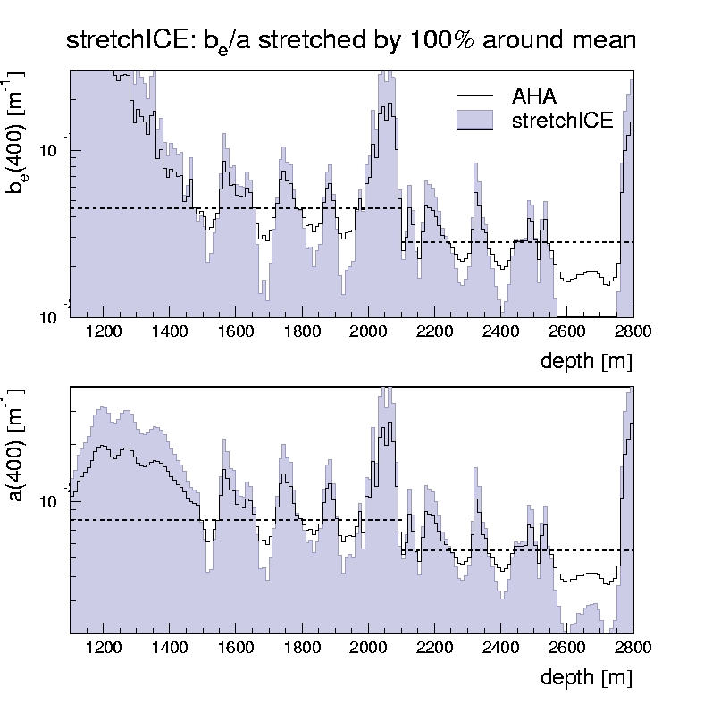
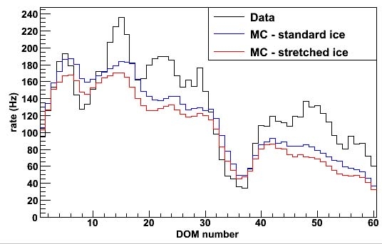
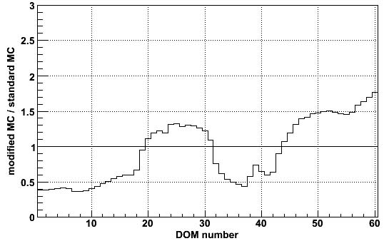
9.1 Stretched Ice Model . . . . . . . . . . . . . . . . . . . . . . . . . . . . . . . . . . . . . 139

9.2 Systematic Error of Ice Properties . . . . . . . . . . . . . . . . . . . . . . . . . . . . . 139

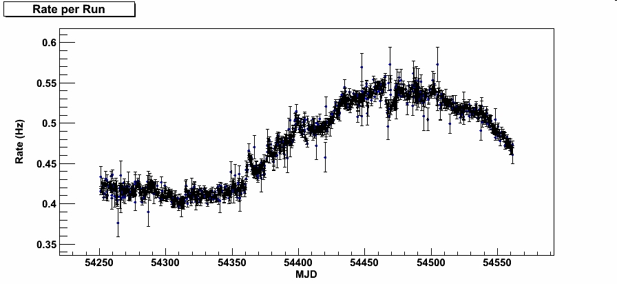
9.3 Seasonal Variation in Data Rate . . . . . . . . . . . . . . . . . . . . . . . . . . . . . . 141

10.1 Comparison of Results with Previous Limits . . . . . . . . . . . . . . . . . . . . . . . . 145

10.2 Opacity of the Universe to High Energy Photons . . . . . . . . . . . . . . . . . . . . . 148

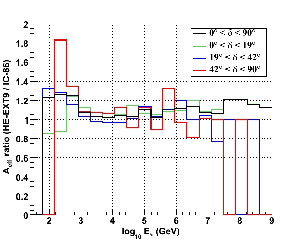
10.3 Neutrino Effective Area for Multiple Detectors . . . . . . . . . . . . . . . . . . . . . . 150

xiii

B.1 IceCube Configurations . . . . . . . . . . . . . . . . . . . . . . . . . . . . . . . . . . . 164

B.2 Neutrino Spectra for 142 Northern Sky GRBs . . . . . . . . . . . . . . . . . . . . . . . 165

B.3 Default Geometry Event Selection . . . . . . . . . . . . . . . . . . . . . . . . . . . . . 166

B.4 Extended Geometry Event Selection . . . . . . . . . . . . . . . . . . . . . . . . . . . . 166

B.5 Effective Areas for the Full Detector . . . . . . . . . . . . . . . . . . . . . . . . . . . . 167

B.6 Discovery Potential of IceCube for GRBs . . . . . . . . . . . . . . . . . . . . . . . . . 169

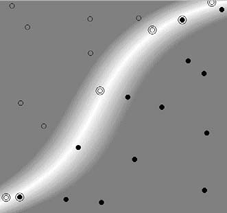
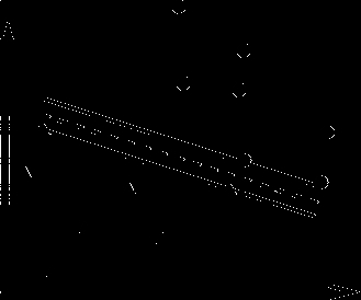
C.1 Hyperplanes in a 2D Support Vector Machine . . . . . . . . . . . . . . . . . . . . . . . 171

C.2 Linear, Fully Separable SVM . . . . . . . . . . . . . . . . . . . . . . . . . . . . . . . . 172

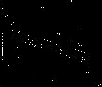
C.3 Linear, Non-Separable SVM . . . . . . . . . . . . . . . . . . . . . . . . . . . . . . . . . 174

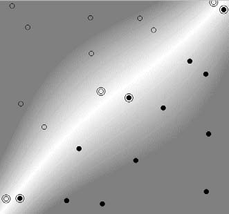
C.4 SVM Kernel Functions . . . . . . . . . . . . . . . . . . . . . . . . . . . . . . . . . . . . 176

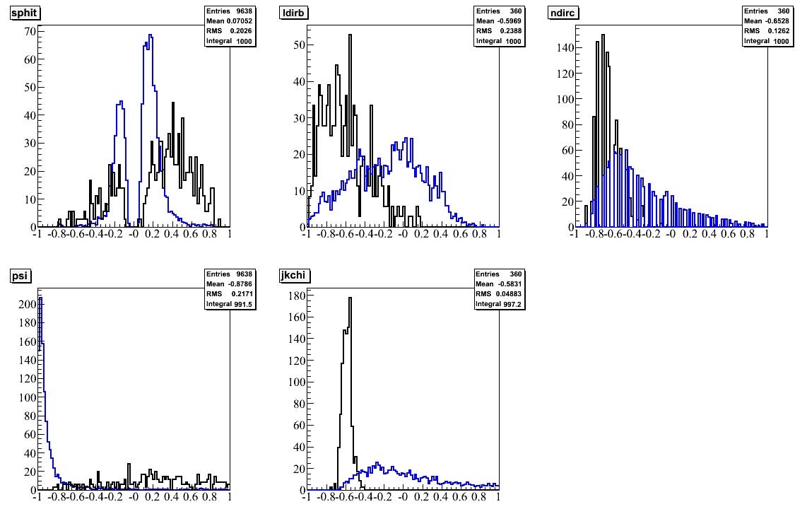
C.5 GRB Feature Vector Distribution . . . . . . . . . . . . . . . . . . . . . . . . . . . . . . 179

C.6 Over-fitting of an SVM classifier . . . . . . . . . . . . . . . . . . . . . . . . . . . . . . 180

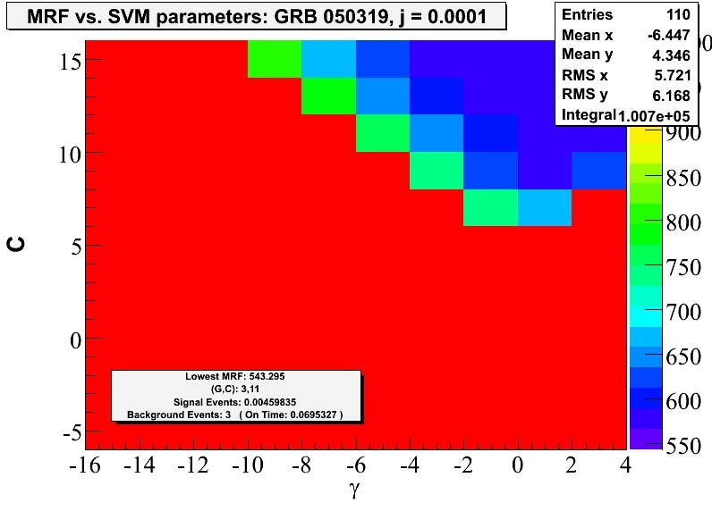
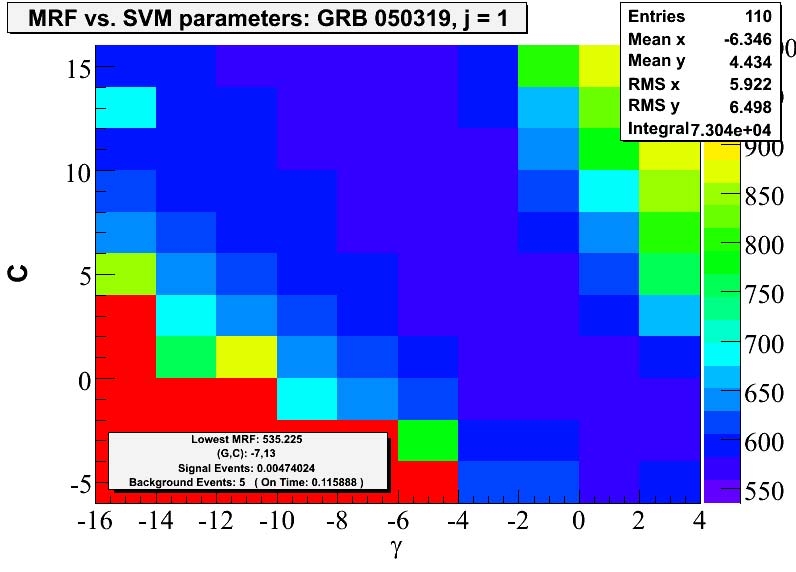
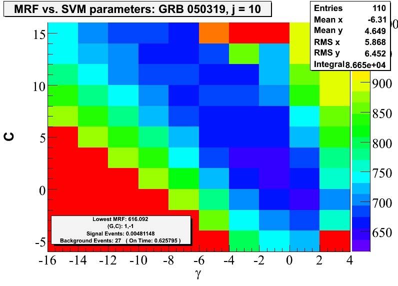
C.7 Grid Search for SVM Optimization . . . . . . . . . . . . . . . . . . . . . . . . . . . . . 181

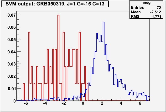
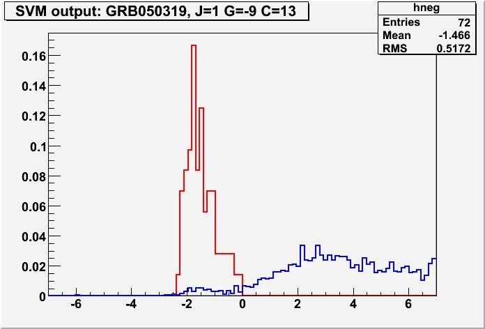
C.8 Effect of Kernel Variation on SVM Output . . . . . . . . . . . . . . . . . . . . . . . . 182

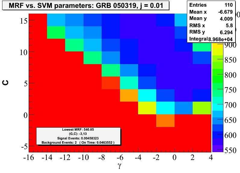
C.9 Global Optimization of SVM Parameters . . . . . . . . . . . . . . . . . . . . . . . . . . 183

Chapter 1

Introduction

High energy neutrinos provide a unique perspective on the cosmos. As neutral and weakly interacting

particles they point back to their sources over all energy ranges and distance scales. This can be

contrasted to cosmic rays which are bent in galactic and intergalactic magnetic fields, or photons,

which can be blocked by intervening matter or attenuated at high energies via pair production with

background light. Thus neutrinos allow us to view the deep universe with a clarity unparalleled in

other channels. In addition, the detection of astrophysical high energy neutrinos would be a clear

signature of sources of hadronic acceleration. Such a detection would have extremely important

consequences in the astrophysics community, as it could explain the origins of the mysterious ultra-

high energy cosmic rays (UHECR). One of the most likely candidates for the production of cosmic

neutrinos are the enigmatic Gamma-Ray Bursts. Extremely brilliant emitters of high energy photons

over time scales ranging from tenths to thousands of seconds, GRBs have a rich observational history

and well developed theories with predictions for neutrino fluxes of energy MeV-EeV.

1.1 The Cosmic Ray Connection

The cosmic rays are composed mostly of protons, with a small fraction of heavier elements

that varies with energy. They are distributed nearly isotropically over the sky and universally follow

a power law spectrum over many decades in energy (see Fig. 1.1). This spectrum falls as E

? 2.7

up to

∼ 4 PeV, where is steepens to E

? 3.7

. This change is spectral slope is known as the knee. Through the

knee, the cosmic rays are thought to be galactic in origin, likely accelerated in supernova remnants

(see section 1.1.1). A good phenomenological description of the steepening is a many-knee model

(poly gonato from Greek) [1, 2]. Each element exhibits a cutoff in its spectrum due to the maximum

acceleration possible in SNR, but heavier elements extend to higher energy. When added together,

the spectrum is well modeled up to ∼ 10

18.5

eV. At this point it hardens to E

? 2.7

again, a feature

known as the ankle. The ultra-high energy cosmic rays above the ankle are thought to be due to

extragalactic sources. At the highest energies they will be suppressed by interactions with the cosmic

microwave background (GZK effect).

Protons accelerated to ultra-high energy will produce neutrinos through interactions with

surrounding matter. While the protons will be isotropized by intervening magnetic fields (except at

the very highest energies), the neutrinos will stream straight to the Earth. If we can detect these

high energy neutrinos we will unveil the sources of the UHECR.

1.1.1 Fermi Acceleration of Particles

First proposed in 1949, Fermi suggested that charged particles would elastically scatter off

turbulent variations in magnetic fields, stochastically gaining energy. Let us follow his work and

determine the energy change in each interaction. A further description may be found in [4].

Let us assume that the “magnetic mirrors” move randomly and have a characteristic velocity

V while the particle moves with velocity v. We further assume that the clouds of gas containing

these mirrors are massive and thus are essentially unaffected by collisions with particles. We thus

choose the center of momentum frame of the cloud for our discussion. The particle energy incident

at angle θ with the magnetic mirror is then given by

= γ(E + Vp cos θ)

(1.1)

and the momentum normal to the mirror surface is

= p

cos θ

= γ

p cos θ +

(1.2)

In the elastic collision, energy is conserved in the center of momentum frame, and momentum is

inverted. In the observer’s frame this yields a final energy

??? ????? ???????????? ?? ?????? ????

????? ? ???? ??? ?????? ??? ???????? ?? ??? ?????? ??? ?????? ?? ?????? ???? ??

???????? ?? ??? ??? ???? ?????? ?? ??? ?? ???????? ?????? ????? ???? ?? ?

?????? ??? ??? ??????? ?? ?????????? ?????? ????????? ?? ??????? ?? ? ? ?????? ??

??? ??? ??????? ?? ?????? ????? ?? ??? ?????? ???? ?? ??? ??????? ???????? ???

??????????? ?? ?????? ???????? ????? ?? ??? ?? ?????? ??? ???? ???? ???? ? ? ???

???????? ???? ? ??? ?? ????????? ???? ??????? ???????? ??????? ??? ??????????

??? ????? ?? ?????? ?? ?? ????????? ??????????? ?? ???? ? ?? ?? ?? ??? ?????? ??

????????? ??? ? ? ????????????

???

????? ???????????? ?? ?????? ????

?? ????? ???????????? ??????? ????????? ??? ??????????? ?????????? ??????? ?????

??????? ?? ???????? ???? ??????????? ?? ??? ??????? ?? ? ??? ??????? ??? ???

??? ????????? ??? ?? ???????? ?????? ??????????????? ???? ???????? ????????

Figure 1.1: The cosmic ray energy spectrum at earth. Below the knee, the cosmic rays are

thought to be galactic in origin. In the high energy tail, sources are unknown. (from [3])

= γ(E

+ Vp

)

(1.3)

= γ

2V v cos θ

(1.4)

The change in energy is thus

? E =∆E =

2V v cos θ

+ 2

(1.5)

where we have expanded to second order in V/c. Note that to first order the total energy change

tends to zero, as the gain of head-on collisions is canceled by the loss in following collisions. This is

not quite true, as the rates are proportional to the relative velocities of approach, v + V cos θ and

v ? V cos θ. Thus, slightly more head-on collisions occur, yielding a net increase in energy. Averaging

over all angles of incidence yields a total fractional energy change

∆E

(1.6)

This is Fermi’s famous result, that the energy increases only with the 2nd order of V/c. While this

mechanism indeed produces a power law, it is deficient for explaining the highest energy cosmic rays.

The velocities of the clouds containing the mirrors are typically small relative to light, and the mean

free path of cosmic rays is large, hence it would take an extremely long time to accelerate particles to

the appropriate energies. Given turbulence on a sufficiently small scale such as in supernova remnants

this can be overcome. However, we must also account for ionization losses which scale with energy.

When combined, 2nd order Fermi acceleration cannot account for the cosmic ray spectrum.

If we could somehow find a situation in which every collision was head-on, Eq. 1.5 tells us

that the energy would increase in every case and be proportional to V/c. This is the so-called 1st

order Fermi acceleration. This can be achieved if strong shocks exist in the accelerator. There are

two approaches to the problem; considering the diffusion equation that governs the evolution of the

momentum distribution around the shocks [5], and following the behavior of individual particles [6].

We adopt the latter approach in the following.

Shocks occur when exploding gas (from e.g. a supernova) travels faster than the sound speed

of the medium. These shocks travel through regions containing high energy particles moving in

magnetic fields. The particles barely notice the presence of the shocks since they have much higher

velocities and the shocks are thin compared to their gyroradii. Elastic scattering of the particles in

turbulent magnetic fields both in front of and in the wake of the shock isotropizes their velocities.

Thus, for a shock traveling at speed U, in the shock rest frame the upstream particles will appear to

be approaching with that same speed. Energy, mass, and momentum must be conserved across the

shock front, and this allows us to determine the resulting compression. For strong shocks the relation

between the gas densities in the downstream and upstream regions is given by

? 1

(1.7)

Here γ

is the ratio of specific heats and is 5/3 for a fully ionized plasma. Thus the compression

ratio is a factor of 4. Conservation of mass implies

= ρ

(1.8)

In the shock rest frame, the upstream gas has velocity ? U while the downstream gas has velocity

? 1/4U. We now consider both upstream and downstream regions individually. In the rest frame

of the upstream gas (adding U to each side), the downstream particles approach the shock front

with velocity 3/4U. Similarly, in the rest frame of the downstream particles (adding 1/4U to each

side), the upstream particles approach the shock front with speed 3/4U. Due to the compressive

properties of the shock, particles have head-on collisions no matter whether they are in the upstream

or downstream regions, and those collisions occur with the exact same velocity relative to the shock.

This is shown schematically in Fig. 1.2.

We can determine the fractional energy increase in each shock crossing in much the same way

, v

shock

downstream

upstream

upstream rest frame

downstream rest frame

shock rest frame

= 1/4 v

= |U|

= 3/4 U

at rest

= 3/4 U

at rest

Figure 1.2: Schematic showing the process for 1st order Fermi acceleration across shock

fronts. Top left panel depicts the shock propagating with velocity U through a high energy

plasma. Top right panel shows the rest frame of the shock and the compression between

the upstream and downstream regions. Because the velocities are isotropized by magnetic

fluctuations, the relative velocity of the upstream region is given by U. Bottom left and

right panels show the rest frame of the upstream and downstream regions, respectively. In

each case, particles crossing the shock front undergo head-on collisions with gas at relative

velocity 3/4U.

as for the 2nd order mechanism. Encountering gas of velocity V = 3/4U, the energy increases by

= γ(E + p

V )

(1.9)

In all the above we have taken the shocks to be non-relativistic while the particles are. Taking this

into account, we arrive at

∆E

cos θ

(1.10)

We average over incidence angles and probabilities to find

∆E

? =

(1.11)

for each full crossing from the upstream to the downstream region and back. If we denote the energy

increase in each interaction by E = βE

then

β =1+

(1.12)

Let us now assume that after each collision the particle has a probability P to pass through the shock

front again. After k collisions we will then have a number of particles N = P

with characteristic

energy E = β

. These can be related through

ln P

ln β

(1.13)

Since N actually represents the number of particles with at least energy E, we then write the differ-

ential energy spectrum as

N(E)dE ∝

ln P

ln β

り 1

(1.14)

We now determine the re-crossing probability P . The number of particles crossing the shocks

is given by 1/4nc [4], where n is the number density. Conversely, in the downstream region, particles

are carried away from the shock front (top right panel of Fig. 1.2). This occurs at a rate 1/4nU. So

the loss per unit time is given by U/c. We then have

P =1 り

(1.15)

We combine Eqs. 1.12 and 1.15 and plug into Eq. 1.14 to find

N(E)dE ∝ E

り 2

(1.16)

Thus we naturally arrive at a power law spectrum consistent with the observed and pervasive cosmic

rays

. We must note, however, that there is a limit to how much acceleration is possible with this

mechanism. Although much more efficient than 2nd order Fermi acceleration, the process is still

slow and must combat energy loss processes. Taking this into account, we find that this process

can account for cosmic ray acceleration in supernovae up to the knee. However, it is not possible to

produce the highest energy cosmic rays with this method. To do so, we must employ much higher

magnetic fields or larger acceleration regions

. We depict this in Fig. 1.3 and note that gamma-ray

bursts are one of the few source classes in which the conditions for UHECR acceleration are indeed

met.

Steepening to an E

り 2.7

spectrum is thought to be due to losses in the intervening space.

We should also note that this discussion has been limited to non-relativistic shock acceleration. The relativistic

case is much more complicated and we do not discuss it in detail here. It has the property however, of rapidly increasing

the energy of particles with each crossing of the shock front and is thus appropriate for UHECR acceleration.

Figure 1.3: The famous Hillas diagram illustrating the relationship between magnetic

fields and source size necessary to accelerate nuclei to ultra-high energies via the Fermi

mechanism. (adapted from [7])

1.2 Previous Work

Previous searches for high energy neutrino emission from gamma-ray bursts have been con-

ducted using data collected with the AMANDA and IceCube detectors. A variety of search strategies

have been employed covering a range of emission models and detection channels. Triggered searches

in the muon channel [8, 9, 10], triggered and rolling searches in the cascade channel [11], and anal-

yses dedicated to single, spectacular bursts [12, 13] have all failed to detect neutrinos from GRBs.

Upper limits have been set, but to date none exclude the most popular scenarios. We build on this

previous body of work in the analyses presented in this thesis and place all results in context in our

conclusions.

1.3 Organization of the Thesis

• Chapter 2 reviews the history of gamma-ray burst observations and presents the phenomeno-

logical framework that has been developed to explain them. We then describe the production

of neutrinos in GRB explosions through photomeson interactions and detail resulting spectra

occurring from the various phases of the emission.

• Chapter 3 describes the ways in which high energy astrophysical neutrinos may be detected

at the earth. The process is followed through interaction, lepton production, and subsequent

emission of

Ceˇ renkov radiation. Optical properties of the detection medium are considered. We

discuss how the arrival times and amplitudes of the emitted light may be used to reconstruct

events, and present the algorithms used in these reconstructions.

• Chapter 4 describes the satellites that observe the photon flux from GRBs and localize their

positions. The AMANDA and IceCube neutrino detectors are then presented, including layout,

hardware, and data acquisition systems.

• Chapter 5 explains the selection criteria for the inclusion of observed GRBs in our search. We

describe the blinding procedure and the determination of emission windows. The spatial and

temporal information for all bursts in our analyses are listed.

• Chapter 6 explains the process of creating simulated signals and backgrounds. The generation

of primaries is described, as well as the modeling of propagation through the atmosphere and

earth, energy losses, interaction, and the detector response to the emitted light.

• Chapter 7 presents a stacked search for muon neutrinos from GRBS using the AMANDA-II

detector. 85 GRBs observed in the northern hemisphere in 2005-2006 are considered. Event

selection and optimization of background rejection are presented in detail.

• Chapter 8 describes a search for muon neutrino emission from 41 GRBs using the 22-string

configuration of the IceCube detector. An unbinned likelihood method is utilized for the first

time in stacked searches for GRBs, maximizing the sensitivity of the analysis.

• Chapter 9 reviews the sources of systematic error in the analyses presented. Contributions from

theory, ice properties, and hardware are considered, as well as the effect of seasonal variation

in the atmospheric muon rate.

• Chapter 10 presents a summary of the work conducted in this thesis and places it in the context

of previous results. Prospects for the future are discussed.

Chapter 2

Gamma-ray Bursts

Gamma-ray Bursts (GRBs) are the most energetic events in the universe, outshining all other sources

over their short emission windows. Initially thought to be galactic in origin due to the fluxes observed,

they are now known to occur at cosmological distances. They are one of the prime candidates for

the acceleration of the highest energy cosmic rays and concurrent astrophysical neutrinos.

2.1 History

Gamma-ray bursts were discovered as a byproduct of efforts to enforce the partial test ban

treaty of 1963. This treaty prohibited the testing of nuclear weapons underwater, in the atmosphere,

and in space. The Vela satellites [14] were designed to detect the gamma radiation from such a

nuclear detonation. The satellites were operated in pairs on opposite sides of a high circular orbit

and timing information was used to determine the direction of sources. During data taking by Vela

5a and 5b in 1969, a strange phenomenon was discovered

; short, intense bursts of γ-rays from

outside their orbits rather than within. This topology meant that the sources were astrophysical

rather than terrestrial. When the data was declassified in 1973, the observations of 16 such bursts

were published [15]. Shortly thereafter, a collimated gamma-ray telescope aboard the OSO-7 satellite

was able to confirm the direction of one of the events [16]. The IMP-6 was able to measure spectral

characteristics of the bursts

and determined that the emission peaked in γ-rays and was thus not

just the high energy tail of some x-ray phenomenon [17]. These observations, all in rapid succession,

spurred a wealth of theoretical papers about the sources of these bursts. Unfortunately this was the

though it was not noticed in 1972 when the backlog of non-nuclear detonation γ-ray events began to be analyzed

using a hard x-ray detector intended to study solar flares

beginning of an experimental dark age that would not see an end for nearly 20 years.

Figure 2.1: The Vela 5 satellite system. On the left is the Vela 5a and 5b pair joined

before launch. On the right is the Vela 5b satellite in low Earth orbit

The Burst and Transient Source Experiment (BATSE) [18] was launched aboard the Compton

Gamma Ray Observatory (CGRO) satellite on April 5, 1991. This was the first experiment dedicated

to the observation of gamma ray photons associated with transients. Its energy range (20 keV - 1

MeV) and all-sky field-of-view allowed it to detect GRBs at an average rate of 1/day throughout its

9 year mission, observing 2704 GRBs in total. This high rate of detection quickly increased statistics,

and studies were able to be conducted on the distributions of the GRB population. It was found that

the durations of GRBs follow a bimodal distribution [19]; so-called “short” bursts with a duration

? 2 s and “long” bursts with a duration ? 2 s. This distribution can be seen in Fig. 2.2. The short

bursts were found to display harder energy spectra than the long, leading to the supposition that

different underlying processes were at work in the 2 classes. The second major finding was in the

spatial distribution of the GRB population. Until this point, most people had thought that the

bursts must be galactic in origin, due to the fluxes observed (some theories even place the source of

the GRBs in the Oort Cloud). It was therefore a great surprise when BATSE observed that GRBs

are distributed isotropically both in number and in fluence [20] (see Fig. 2.3. In a galactic source

model, the brightest bursts would be distributed along the galactic plane. This lack of clustering

gave evidence that GRBs are cosmological phenomena, which implied huge energies of 10

り 10

ergs in the case of isotropic emission from the sources.

Figure 2.2: Distribution of GRB Durations for the BATSE 4B Catalog (through August

1996). Durations are given as T

, the time in which 5% to 95% of the γ-ray emission

occurs. The bimodal distribution separates GRBs into 2 classes; long and short (based on

data from [21])

The hypothesis of cosmological origin was confirmed by the BeppoSAX satellite [22] in 1997.

BeppoSAX was able to localize GRBs with arcminute precision, and more importantly, was able to

distribute that information to ground-based observatories much more rapidly than had previously

been achieved. In addition, they were able to make x-ray observations of GRB afterglow. These

multi-wavelength afterglow observations led to the first observation of an optical counterpart to a

GRB at cosmological distance [23].

The Swift satellite [24, 25] (see section 4.1.1), launched in 2004 opened a new window on

understanding GRBs. It was designed to have rapid slewing capability and incorporates γ-ray, x-ray,

+90

-90

+180

-180

2704 BATSE Gamma-Ray Bursts

-7

-6

-5

-4

Fluence, 50-300 keV (ergs cm

-2

)

Figure 2.3: Spatial Distribution of the full BATSE GRB sample. The isotropic spatial

distribution in both number and fluence implies cosmological origins. (from [18])

and ultraviolet detectors onboard. This has allowed detailed studies of the transition between the

prompt and afterglow emission phases and the first measurements of afterglow emission from short

GRBs [26]. Rapid dissemination of (usually) arcsecond localizations to ground-based telescopes

results in redshift measurements for ∼ 25% of all bursts. It has been found that the GRB population

extends to higher redshifts than imagined, with observed distances up to z=6.7 [27].

After nearly a decade without a full-sky GRB detector, the Fermi Gamma Space Telescope [28]

(formerly GLAST) was launched in July of 2008. A true successor to CGRO, Fermi possesses both

a wide field Gamma-ray Burst Monitor (GBM) and a more focused, higher precision detector (the

Large Area Telescope, or LAT). The LAT is analogous to the EGRET experiment aboard CRGO,

extending the energy range to 300 GeV. Fermi is able to slew to point the LAT at some GRBs

detected by the GBM, thus yielding a huge potential range of energies for GRB observations. This

has led to the detection of >10 GeV photons from bursts [29], raising new questions as to the source

physics. With a detection rate of ∼ 200/yr Fermi will continue to provide valuable new data in the

quest to understand the mysteries of GRBs.

2.2 Fireball Model

Long GRBs are thought to be caused by the core collapse of massive stars into black holes [30,

31]. This hypothesis is strengthened by the association of some long GRBs with abnormal type Ic

Supernovae (SNe)

. The first such correlation was between GRB980425 and SN1998bw [32] with

several other observations strengthening the connection to date. Long GRBs are always observed to

occur in star-forming regions. Short GRBs, on the other hand, are thought to be associated with

the merger of two compact objects (e.g. neutron stars) [33]. In either case, the accreting matter

is thought to spin rapidly, creating a disk [34]. At some point, the radiation pressure exceeds the

gravitational infall, and an explosion occurs, ejecting an e

, γ, and baryon plasma along the rotation

axis, with this fireball being fed by rapid accretion of matter from the disk. This wind accelerates to

relativistic velocities and randomizes and dissipates energy via internal shocks. It is thought that the

observed γ-rays are the result of synchrotron radiation from the accelerated electrons in the very high

magnetic fields of the burst environment [35, 36]. Let us consider the observations that lead to this

fireball phenomenology in order to better understand the physics of GRBs and why it is reasonable

to expect high energy neutrino emission.

2.2.1 Energy Spectra

The energy spectra of most GRBs are well described by the Band function [37], which models

the low energy component as a power law with exponential cutoff, smoothly transitioning to a steeper

power law at higher energies. While the fit is purely empirical and makes no claims with regards to

the burst physics, it is in agreement with a model of synchrotron emission from accelerated electrons

which then undergo cooling above some break energy. We simplify the picture slightly by taking

the photon spectra to be a broken power law, with the normalization chosen such that the fluence

integral matches that fit by the Band function.

This class of supernovae are known as hypernovae and are characterized by smooth spectra, higher than usual

energy, and strong radio emission.

dN(E

)

= f







(α

り β

)

り α

for E

< ?

り β

for E

≥ ?

(2.1)

dN(E

)

(2.2)

where F

is the measured photon fluence. The break energy varies for each burst, but has a typical

value of ?

∼ 250 keV

. Long bursts tend to have spectral indices scattered around α

∼ 1 and β

∼ 2

while short GRBs are harder by one power in energy on average.

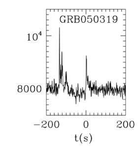
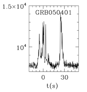
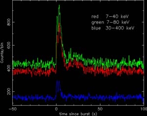
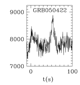
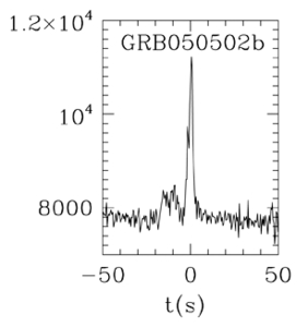
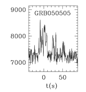
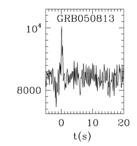
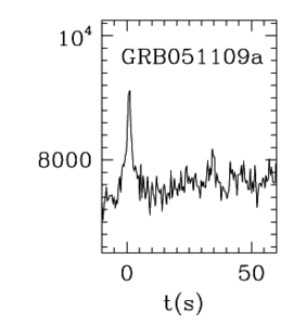
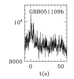
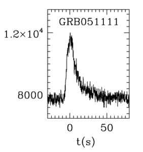
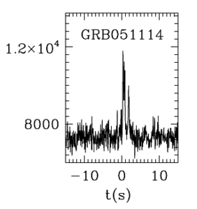
Figure 2.4: Lightcurves for several gamma-ray bursts. Note that all bursts exhibit unique

temporal characteristics and some have short timescale variability. (from [25])

We note that the Swift detector (see section 4.1.1) is transparent to γ-rays above 150 keV and thus does not detect

the spectral break for the majority of GRBs it observes.

2.2.2 Compactness

GRBs experience variability on millisecond timescales (see Fig.2.4). The finite speed of light

places constraints on the source size. For a source of diameter d, any temporal variability of scale

smaller than ∆t ∼

will be smeared out by delays in travel time. This means that the compact

progenitor must satisfy:

GRB

c∆t

(2.3)

For observed timescales of ∆t ∼ 0.01 s, this gives a characteristic radius of R

GRB

? 1500 km.

For comparison, the radius of a neutron star is typically ∼ 12 km. In the case that the compact object

is a black hole, the source size can be defined by the Swartschild radius:

Swartschild

2GM

(2.4)

This relation yields an upper limit to the possible source mass of a GRB progenitor, supposing that

it is a black hole.

GRB

∼ 2 × 10

kg ∼ 1000M

(2.5)

The isotropic distribution observed by BATSE (see Fig. 2.3) implies that GRBs are cosmo-

logical in nature. Coupled with the measured fluences F

and the standard Λ

CDM

cosmology, this

leads to high corresponding energies at the source, E

iso

, of ∼ 10

り 10

ergs. Given that GRBs have

durations spanning from 0.1 s to >100 s, this results in luminosities, L

iso

of ∼ 10

り 10

erg/s. Here

we assume isotropic emission of the energy. If we take the typical photon energy in a GRB to be ?

then we can determine the number density of photons in the source:

iso

4πR

c ?

(1 + z)

≈ 1.5 × 10

り 3

(2.6)

The above implies that the photons should be thermalized due to the high optical depth of the

This is reasonable given that emission tends to peak at the break energy, and that most of the photons will be

emitted at the peak.

plasma, which is at odds with the observed high energy emission well above the pair production

threshold. This is known as the compactness problem.

In order to resolve this apparent crisis, we note that given the mass limit imposed by Eq. 2.5

and the observed luminosities of O(10

) erg/s, the progenitor far exceeds the Eddington limit and

thus must drive a wind from the surface. We consider the case that the expansion is highly relativistic

and thus the photons will appear to be emitted in a cone of opening angle θ due to aberration. The

geometry is illustrated in Fig. 2.5. The observed time delay between spectral features is now given

∆t

obs

∆t(c り v cos θ)

(2.7)

t (c -

cos

θ)

cos

Figure 2.5: Effect of relativistic aberration on time variability. The relativistically ex-

panding plasma is beamed into an opening angle θ. An observer situated along the line of

sight will observe a different time between spectral features than is intrinsic to the source.

We write the expansion velocity v in terms of the Lorentz factor 㡇 and Taylor expand (assuming

large 㡇) to get

v ≈ (1 㡇

2㡇

(2.8)

Similarly, the opening angle will be small so the same technique may be applied. Combining terms

yields

∆t

obs

≈ ∆t

2㡇

(2.9)

Since the beaming angle θ is inversely related to the Lorentz factor, we arrive at

∆t

obs

∆t

㡇

(2.10)

GRB

≈ c∆t

obs

㡇

(2.11)

Similarly, the intrinsic luminosity of the GRB is reduced by a factor 㡇

and the individual pho-

ton energies by a factor 㡇. We determine that the plasma becomes optically thin for 㡇

> 100.

Such a Lorentz factor also places the bulk of photons below the pair production threshold. Direct

measurements by Molinari et al. [38] give 㡇 ∼ 400.

2.2.3 Emission Mechanism

Assuming now an outflow with 㡇 ≥ 100, the jet must collide with the ISM and slow down.

While this external shock may account for observed afterglow emission, the time and distance scales

on which it occurs preclude it from being the cause of the prompt emission as it cannot produce

the observed temporal variability. We turn instead to internal shocks within the jet. While the jet

moves with a bulk Lorentz factor 㡇, individual ejections from the progenitor will have varying speeds.

When faster shells overtake slower shells, shocks will occur. At these shock fronts, electrons may be

accelerated via the Fermi mechanism (outlined in section 1.1.1). Due to the shock compression of

the fluid and the high velocity of expansion, the acceleration is both very efficient and fast. These

electrons then emit photons via synchrotron (and perhaps inverse Compton) radiation, resulting in

the observed keV-GeV emission. Such an internal shock acceleration scenario both accounts for rapid

temporal variability as well as a power law energy spectrum. It is natural that protons would also

be accelerated in these shocks, potentially leading to neutrino production.

2.2.4 Collimated Emission - Reducing the Energy Budget

While the energy budget for GRBs is extreme, it may be reduced if the emission is collimated.

In this case, the required energy is reduced by a factor Ω/4π where Ω is the opening angle of

the collimated jet. This would be experimentally observable by a temporal break in the afterglow

emission. The reason for this break comes from the interaction between the relativistic beaming effect

and the intrinsic beaming of the jet. The highly relativistic outflow from the GRB is Lorentz-beamed

into an angle of 1/㡇. As the fireball propagates through the interstellar medium (ISM) it is slowed

and the bulk Lorentz factor decreases, thus increasing the beaming angle. At some point, the outflow

will have slowed enough such that 1/㡇 > Ω and a flux deficit will be observed as a steepening of the

spectra. This jet break has a unique signature in several ways. First, it is achromatic - that is, since

it is a purely hydrodynamic effect, it affects all wavelengths equally. Second, it does not impact the

physics of the burst itself, so no effect on the electron or photon spectral index is expected. Further

details may be found in [39, 40].

Clear evidence of multi-color optical breaks with consistent radio data was observed in the

case of GRB990510 [41], among others (see Fig. 2.6). Based on the observed temporal jet breaks for

a sample of several tens of bursts, Frail et al. [42] and Bloom et al. [43] calculated the corresponding

jet collimation angles and GRB energies. They found that all GRBs in the sample were narrowly

clustered around emission energies of E

∼ (5×10

㡇 1.3×10

ergs, as seen in Fig. 2.7. Thus, GRBs

have an energy budget on par with bright Supernovae, suggesting a correlation, and the observed

variances in luminosity and fluence can be attributed to differences in the jet opening angle rather

than intrinsic properties. Furthermore, this suggests that the true rate of GRBs is much higher, as

we only observe bursts with collimated emission along line of sight.

While the idea of beamed emission is attractive in that it reduces the energy budget of GRBs

to levels more in line with other astrophysical phenomena (e.g. supernovae), recent data calls these

conclusions into question. It was expected that Swift, with its multi-wavelength observational capa-

bilities, would measure jet breaks for many GRBs. This has not turned out to be the case however,

with very few bursts displaying temporal breaks that are consistent with the jet break model. The

current experimental and theoretical status of jet breaks is more fully covered in [44].

–5–

Fig. 1.— Optical light-curves of the transient afterglow of GRB 990510. In addition to

photometry from our group (filled symbols – see Table 1), we have augmented the light

curves with data from the literature (open symbols). The photometric zero-points in Landolt

V -band from our group are consistent with that of the OGLE group (Pietrzynski & Udalski

1999b) and the I -band zero-point is from the OGLE group. Some R-band measurements

were based on an incorrect calibration of a secondary star in the field (Galama et al. 1999)

and we have recalibrated these measurements.

Figure 2.6: Observation of achromatic jet breaks in GRB990510. The wavelength inde-

pendence of the break times agrees with the jet break model. (from [41])

Figure 3. The distribution of the apparent isotropic γ -ray burst energy of GRBs with known

redshifts (top) versus the geometry-corrected energy for those GRBs whose afterglows exhibit the

signature of a non-isotropic outflow (bottom). The mean isotropic equivalent energy ?E

iso

(γ )? for

17 GRBs is 110 × 10

erg with a 1-σ spreading of a multiplicative factor of 6.2. In estimating the

mean geometry-corrected energy ?E

? we applied the Bayesian inference formalism

and modified

to handle datasets containing upper and lower limits.

Arrows are plotted for five GRBs to indicate

upper or lower limits to the geometry-corrected energy. The value of ?log E

? is 50.71±0.10 (1σ) or

equivalently, the mean geometry-corrected energy ?E

? for 15 GRBs is 0.5 × 10

erg. The standard

deviation in log E

is 0.31

+0.09

㡇 0.06

, or a 1-σ spread corresponding to a multiplicative factor of 2.0.

Figure 2.7: Calibrated GRB energy in the case of beamed emission. Upper panel shows

calculated isotropic equivalent energy for GRBs with measured redshift. Lower panel

shows energy after taking into account jet collimation angle Ω calculated from jet break

times. (from [42])

2.3 Neutrino Production

If hadrons (typically protons) are accelerated along with electrons in the fireball phenomenol-

ogy described above, neutrinos will be produced due to subsequent interactions. The energy spectra

of these neutrinos will depend on the environment and type of these interactions.

2.3.1 Prompt Neutrinos

Waxman and Bahcall showed that protons may interact with the internal shock prompt emis-

sion gamma-rays to produce pions via the delta resonance [45].

p + γ → ∆ → n + π

(2.12)

→ p + π

(2.13)

Charged pions decay to neutrinos and associated leptons, while neutral pions produce high energy

photons

→ µ

+ ν

(2.14)

→ ν¯

+ e

+ ν

(2.15)

→ γ + γ

(2.16)

These processes result in a neutrino flavor ratio at the source of (ν

, ν

) =(1:2:0)

Eq. 2.12 indicates that the produced neutrino spectra should track the γ-ray spectra of Eq. 2.1,

as the combined center of mass energy of the interacting proton and photon must exceed the threshold

for production of the ∆-resonance:

This TeV-scale gamma emission is the target of GRB searches by Imaging Air Ceˇ renkov Telescopes such as MAGIC

as well as surface arrays such as MILAGRO.

Here, and in the rest of this thesis, we treat neutrinos and antineutrinos equally. The minor differences in cross-

section are taken into account in signal weighting but we shall not explicitly differentiate.

≥

∆

㡇 m

(2.17)

where primes indicate the co-moving frame of the fireball. We estimate that each of the four final

state particles in the π

decay chain given by Eqs. 2.12 and 2.14 contains equal energy, and that

on average, a fraction ?x

p→π

? ? 0.2 of the proton energy is transferred to pions in each interaction.

Thus each neutrino is expected to possess ∼ 5% of the proton energy.

The condition of Eq. 2.17 indicates that interactions of protons with high energy photons will

produce lower energy neutrinos, and vice versa. For each proton energy, then, the neutrino spectrum

traces the broken power law of Eq. 2.1. Assuming protons are accelerated with the same spectrum

as electrons, we then sum over proton energies to find the resultant neutrino spectra.

dN(E

)

∝







㡇 α

for E

< ?

; α

=3 㡇 β

㡇 β

for ?

≤ E

< ?

; β

=3 㡇 α

(2.18)

We relate the break in the neutrino spectrum to that of the observed photons by converting

Eq. 2.17 to the observer’s frame.

p→π

∆

㡇 m

㡇

(1 + z)

= 7.5 × 10

GeV

(1 + z)

㡇

2.5

MeV

(2.19)

At high energy, the lifetime of the produced pions and muons τ

π,µ

exceeds the synchrotron

loss time t

. This introduces a further cooling break into the neutrino spectrum. t

is dependent on

the energy density of the magnetic field in the jet, U

= B

/8π, and for pions is given by:

4σ

(2.20)

where σ

= 0.665 × 10

㡇 24

is the Thompson cross-section. The magnetic energy density can be

related to the fraction of the internal energy of the plasma that is carried by the magnetic field. We

denote this fraction by ξ

and write

4πR

c㡇

= ξ

int

(2.21)

We determine the collision radius R by noting that the colliding shells of the jet have velocities that

vary by ∆v ∼ c/2㡇

, where, as previously, 㡇 represents the average Lorentz factor of the fireball.

Given the observed time variability t

var

, these shells then collide at a time t

∼ ct

var

/∆v, which

corresponds to a radius R ? 2㡇

var

. The total luminosity is related to the observed photon

luminosity through the electron energy fraction of the jet, L

int

= L

iso

/ξ

. [46, 47]

The pion lifetime is given by

= τ

= 2.6 × 10

㡇 8

(2.22)

Equating Eq. 2.20 with Eq. 2.22 yields the pion energy where synchrotron losses begin to suppress

the neutrino emission. Recalling the each ν

carries 1/4 of the pion energy, and converting to the

observer’s frame, we find

= 10

GeV

1+ z

㡇

2.5

var

0.01 s

erg/s

iso

(2.23)

We note that in the above the equipartition fractions ξ

and ξ

are not measured and no good

theoretical method exists for estimating them. We set them each to be 0.1 in all future calculations.

This estimate is supported by afterglow observations [48]. Muons live about 100 times longer and

thus the energy scale at which their decay products (ν¯

and ν

) begin to be suppressed is a factor of

10 lower. The decay probability is approximately given by the ratio of the cooling time to the decay

time t

/τ

∝ E

㡇 2

and thus we expect the neutrino spectrum to steepen by 2 powers in energy above

(γ

= β

+ 2). Combining with Eq. 2.18 we arrive at

dN(E

)

= f







(α

㡇 β

)

㡇 α

for E

< ?

㡇 β

for ?

≤ E

< ?

(γ

㡇 β

)

㡇 γ

for E

≥ ?

(2.24)

It now remains to determine the normalization f

. The neutrino fluence is proportional to the

measured gamma-ray fluence F

dN(E

)

= x ·

dN(E

)

= x · F

(2.25)

The constant of proportionality x contains several terms. It includes the fraction of jet proton energy

lost to pion production f

, a factor 1/f

that accounts for the fraction of total energy expected in

protons respective to electrons, and a factor 1/8. This final term is due to the fact that only half of

the photomeson interactions produce neutrinos (the others produce π

) and each of those reactions

creates four final state leptons. f

can be estimated from the size of the shocks and the mean free

path for photomeson interactions.

∝

∆R

pγ

= N

int

(2.26)

The number of interactions is related to the photon energy density which is in turn a function of the

GRB luminosity in the comoving frame

. We follow the derivation of [46] and reformulate to ensure

an energy transfer ≤ 1:

= 1 㡇 (1 㡇 ? x

p→π

int

(2.27)

int

iso

erg/s

0.01 s

var

? ?

2.5

㡇

MeV

(2.28)

Here we note that we assume isotropic emission, but also divide by a spherical shell. In the case of beamed emission,

the luminosity decreases, but cancels with the decreased solid angle.

An analytical approximation of the integration over neutrino energies yields a simple relationship

between the neutrino flux normalization and the gamma-ray fluence.

≈

ln(10)

(2.29)

A quasi-diffuse flux may be determined by summing over all bursts in a year and dividing by

the full sky solid angle. This was done by Waxman and Bahcall, assuming each GRB followed a

spectrum calculated from averages of the BATSE population [49]. Assuming 1000 GRBs per year

based on the BATSE rates, they calculated the diffuse flux shown in Fig. 2.8. This will hereafter be

referred to as the Waxman-Bahcall prompt GRB flux. The normalization is comparable to what one

would get assuming that all the ultra-high energy cosmic rays originate from GRBs. The average

parameters used in this calculation are shown in Table 2.1.

reduction of the flux happens above E

[Eq. 23] due to

synchrotron radiation by pions.

3456789

?13

?12

?11

?10

WB Limit

ICECUBE

burst

(head)

(shocks)

(head)

flux (10

bursts/yr)

atmospheric

[log10(GeV/cm s sr)]

E [log10(GeV)]

−1

(stellar)

pp (shocks)

FIG. 1: Diffuse muon-neutrino flux E

㡇 1

, shown as solid

lines, from sub-stellar jet shocks in two GRB progenitor mod-

els, H (r

12.5

) and He (r

), each for two sets of shock/jet radii

and overlying envelope masses (with similar curves for ν

, ν

and ν

). These neutrinos arrive as precursors (10-100 s be-

fore) of γ -ray bright (electromagnetically detectable) bursts,

or as the sole signal in the case of γ -ray dark bursts. Also

shown is the diffuse neutrino flux arriving simultaneously with

the γ -rays from shocks outside the stellar surface in observed

GRB (dark short-dashed curve); the Waxman-Bahcall (WB)

diffuse cosmic ray bound (light long-dashed curves); and the

atmospheric neutrino flux (light short-dashed curves). For a

hypothetical 100:1 ratio of γ -ray dark (in which the jets do not

emerge) to γ -ray bright collapses, the neutrino fluxes would

be 100 times higher than those plotted here.

and this might serve as a diagnostic of the sub-surface jet

depth (or the overlying material). For a solar mass above

the jet head (distributed over 4

νN interactions becomes larger than unity at energies

? 2.5 × 10

GeV in the H case and

GeV in the He case (seen as a cut-off in the lower set of

He curves). Typically 80% of the

to the secondary lepton:

to ν’s, however, they are subject to severe synchrotron

and inverse Compton losses and do not contribute sub-

stantially to lower energy flux.

The diffuse fluxes are based on a conservative estimate

of the source density from the observation that

GRB are known to occur per year over the entire sky,

based on γ-ray detections. If these are attributed to mas-

sive stellar collapses, each GRB should be preceded by

neutrino percursor events, starting tens of seconds (typ-

ically ∼ 30 s [8]) before the

flux from all of these (

given by the solid curves in Fig. 1. (Considering mass-

mixing along the way to Earth from

of flavors as observed from earth should become unity).

The number of neutrino bursts and correspondingly the

diffuse neutrino flux may be up to a factor 100

than what is shown in Fig. 1, if the ratio of the number

of buried jets which do not emerge (

to that of those which do emerge is 100

The number of muon neutrino events, in a km

tector (IceCube [14] e.g.), from a single GRB at redshift

z = 1 with buried jet of duration ∆

0.003 in the r

12.5

(H) and in the

Figure 2.8: Diffuse muon neutrino flux predictions for the prompt and precursor emis-

sion phases. 1000 GRBs/yr. are assumed. Black dashed-line indicates the prompt flux

calculated with average parameters measured by BATSE. Solid black lines correspond

to precursor neutrino predictions for progenitors with a hydrogen envelope (H) and no

envelope (He) for varying shock and jet radii. Fluxes are shown at the source and will be

reduced by a factor of 2 at Earth due to oscillations. (from [50])

Photon Parameter Average Value

1 MeV

GeV

iso

erg/s

㡇

315

var

0.01 s

0.1

Table 2.1: Average parameters used to calculate the Waxman-Bahcall diffuse GRB neu-

trino flux for the prompt emission phase.

2.3.2 Precursor Neutrinos

The relativistic jets that are thought to be responsible for the prompt photon emission of

GRBs must first penetrate the sub-stellar environment of the progenitor. In this region, no photon

emission is expected as the star is highly optically thick. However, shock-accelerated protons may

interact with thermalized photons and nucleons of the jet as well as with cold nucleons in the stellar

plasma to produce neutrinos [50]. This so-called precursor emission occurs at smaller radii and lower

Lorentz factors than the observed prompt photons.

Neutrinos from pγ interactions both in the jet and in the surrounding plasma will be highly

suppressed due to the extreme magnetic fields of the progenitor and the subsequent synchrotron losses

of pions and muons. On the other hand, pp interactions in the unshocked plasma will not be affected

in this way. Assuming a proton injection spectrum with an E

㡇 2

power law, Razzaque et al. performed

detailed simulations of the pp interactions both at the jet head and in the shocks, taking into account

synchrotron as well as inverse Compton losses in order to determine the resulting neutrino flux. This

spectrum cuts off at the energy threshold for pion/kaon production above which no neutrinos from pp

interactions are expected. However, above the ∆ resonance threshold, the suppressed pγ interactions

begin to play a small role. The resulting diffuse flux can be seen in Fig. 2.8 for several progenitor

types and sizes. Further details of the calculations can be found in [50, 51].

2.3.3 Afterglow Neutrinos

X-ray, optical, and radio afterglows have been observed in association with many GRBs. In

the standard picture, these are the result of collisions of the expanding fireball with the circumburst

matter. It has been proposed that the low energy photons are then created via synchrotron radiation

of electrons accelerated in shocks moving inwards. These photons are observed to follow a power

law spectrum which steepens on average by a power of 1/2 above a break energy determined by

the relation between the synchrotron cooling time and the expansion time of the ejecta [51]. These

spectral indices vary between bursts, but are scattered around average values of α

∼ 3/2 and β

∼ 2.

In the hadronic picture, these mildly-relativistic reverse shocks will also accelerate protons

to ultra-high energies [52]. Following the same processes as in the prompt emission scenario, these

protons will interact with the afterglow photons to produce neutrinos. However, since the reverse

shocks happens at large radii of ∼ 10

cm, we do not expect significant synchrotron losses of pions

and muons. In this case, assuming the average photon spectra above, the neutrinos can be described

)

= A







㡇 1

for E

< ?

㡇 3/2

for E

≥ ?

(2.30)

The break energy ?

is related to the photon break energy via Eq. 2.19 and for the observed afterglow

cooling breaks of 0.1 㡇 1 keV, we have

= (0.7 㡇 7) · 10

(1 + z)

㡇 2

GeV

(2.31)

In [52], ?

is fixed at 10

GeV and A

is determined to be 10

㡇 10

GeV cm

㡇 2

㡇 1

by assuming that

the observed flux of ultra high energy cosmic rays is due entirely to GRBs. Neutrinos of energy up to

∼ 10

eV could be produced, although strong suppression is expected above this energy as protons

are not observed above ∼ 10

eV.

2.4 Neutrino Oscillation

Solar Neutrinos were first detected by the Homestake experiment in the late 1960s, using a

large tank of chlorine to capture solar ν

[53, 54]. However, only 1/3 of the neutrinos predicted by

the solar model were detected, leading to the well known “solar neutrino problem”. This was solved

by the Sudbury Neutrino Observatory in 2001 with an experiment that measured the total solar

neutrino flux over all flavors. [55] This was direct evidence of the oscillation between neutrino flavors

that would occur if the neutrinos were massive.

The mass eigenstates are mixed via the Maki-Nakagawa-Sakata (MNS) matrix to produce the

flavor eigenstates:



















㡇 iδ

㡇 s

㡇 c

iδ

㡇 s

iδ

㡇 c

iδ

㡇 c

㡇 s

iδ



















(2.32)

where c

= cos θ

and s

= sin θ

. The phase δ is non-zero in the case that the oscillation is

CP violating. The mass eigenstates propagate in time as plane waves. Since time and length are

equivalent, we may write

|ν

(L)? = e

㡇 im

L/2E

|ν

(0)?

(2.33)

and since these eigenstates have different masses, they will propagate at different speeds. Because

they are superpositions of the flavor eigenstates, this will cause interference between those flavor

states, leading to oscillation over the propagation length. The probability that a neutrino of flavor α

will oscillate to a neutrino of flavor β is then given by

α→β

= |?ν

|ν

(t)?|

∗

αi

βi

㡇 im

L/2E

(2.34)

where U

αi

indicates the MNS mixing matrix between those states. The solution in the full 3 fla-

vor/mass theory is complicated, but includes a term

sin

(

∆m

(2.35)

In the simpler case of a 2 neutrino theory (such as ν

→ ν

oscillation of atmospheric neutrinos,

where the involvement of ν

is very small), the mixing between flavors is given by

α→β

= sin

2θ sin

∆m

(2.36)

where θ and ∆m

are the respective quantities in the 2 neutrino theory.

Cosmological baselines ensure that oscillation occurs and it can be shown that this typically

leads to a conversion of the (1:2:0) source flavor ratio to a flavor ratio at earth of ∼ (1:1:1) [56].

However, Kashti and Waxman showed that π and µ energy losses modify this flavor ratio to (1:1.8:1.8)

at high energies [57]. This conversion takes place over several decades in energy and for GRBs typically

occurs between 100 TeV and 1 PeV.

Chapter 3

Neutrino Detection and Reconstruction

3.1 Interaction

Neutrinos have extremely low cross-sections and interact only rarely via the weak force, even

at high energies [58]. Sometimes, however, a high energy neutrino will interact with an ice or rock

nucleus in or near the detector volume through the charged current interaction

+ N → l + X

(3.1)

where X is the nuclear remnant.

The rate of these interactions depends on energy and angle

of incidence, as shown in Fig. 3.1.

For the analyses presented in this thesis, we consider the case where the daughter lepton of

Eq. 3.1 is a high energy muon. Such daughter muons are highly relativistic and will deviate only

slightly in direction from the primary, with an angular offset given by ψ = 0.7

◦

× (E

/TeV)

㡇 0.7

[59].

At the energies of primary interest (∼ 100 TeV), muons have a range of about 10 km [60]. This has

the fortuitous effect of vastly increasing the effective area of any detector built to view these muons,

as they need not originate in the instrumented volume, merely pass through it.

Neutral current interactions also take place, but these create very different signatures (cascades) in the detector

and are outside the scope of this thesis.

FIGURES

FIG. 1. Cross sections for ν

ℓ

N interactions at high energies, according to the CTEQ4–DIS

parton distributions: dashed line, σ(ν

ℓ

N → ν

ℓ

+ anything); thin line, σ(ν

ℓ

N → ℓ

㡇

+ anything);

thick line, total (charged-current plus neutral-current) cross section.

0.7

0.8

0.9

1.0

1.1

(CTEQ4D)/

(CTEQ3D)

[GeV]

FIG. 2. Ratio of the charged-current cross section shown in Figure 1, calculated using the

CTEQ4–DIS parton distributions, to the charged-current cross section of Ref. [12] calculated using

the CTEQ3–DIS parton distributions.

FIG. 3. Cross sections for ν¯

ℓ

N interactions at high energies, according to the CTEQ4–DIS

parton distributions: dashed line, σ(ν¯

ℓ

N → ν¯

ℓ

+ anything); thin line, σ(ν¯

ℓ

N → ℓ

+ anything);

thick line, total (charged-current plus neutral-current) cross section.

FIG. 4. Cross sections for ν

ℓ

N interactions at high energies, according to the CTEQ4–HJ

parton distributions: dashed line, σ(ν

ℓ

N → ν

ℓ

+ anything); thin line, σ(ν

ℓ

N → ℓ

㡇

+ anything);

thick line, total (charged-current plus neutral-current) cross section.

1.00

1.05

1.10

1.15

1.20

(CTEQ4HJ)/

(CTEQ4D)

[GeV]

FIG. 5. Ratio of the charged-current cross section shown in Figure 4, calculated using the

CTEQ4–HJ parton distributions, to the charged-current cross section of Figure 1 calculated using

the CTEQ4–DIS parton distributions.

FIG. 6. Interaction lengths for neutrino interactions on nucleon targets: dotted line,

charged-current interaction length; dashed line, neutral-current interaction length; solid line, total

interaction length, all computed with the CTEQ4–DIS parton distributions. The dot-dashed curve

shows the charged-current interaction length based on the EHLQ structure functions with Q

held

fixed at Q

= 5 GeV

FIG. 7. Interaction lengths for antineutrino interactions on nucleon targets: dotted line,

charged-current interaction length; dashed line, neutral-current interaction length; solid line, total

interaction length, all computed with the CTEQ4–DIS parton distributions.

FIG. 6. Interaction lengths for neutrino interactions on nucleon targets: dotted line,

charged-current interaction length; dashed line, neutral-current interaction length; solid line, total

interaction length, all computed with the CTEQ4–DIS parton distributions. The dot-dashed curve

shows the charged-current interaction length based on the EHLQ structure functions with Q

held

fixed at Q

= 5 GeV

FIG. 7. Interaction lengths for antineutrino interactions on nucleon targets: dotted line,

charged-current interaction length; dashed line, neutral-current interaction length; solid line, total

interaction length, all computed with the CTEQ4–DIS parton distributions.

Figure 3.1: Upper panels show the νN and ν¯N cross-sections for all flavors as a function

of energy. Dashed line, neutral current interactions; thin solid lines, charged current inter-

actions; thick solid line, total. The curves in these figures are calculated from the CTEQ4

parton distribution functions, however we use updated cross-sections using CTEQ6 in our

analyses. The lower panels show the energy dependent decrease in the interaction length

(in units of cm water equivalent). Dotted line, charge current; dashed line, neutral cur-

rent; solid line, total interaction length. Ignore the dot-dashed line in the lower left panel.

The diameter of the Earth is 1.1 × 10

cmwe, so above 40 TeV, vertical events begin to be

attenuated. As energy increases, one must shift angle towards the horizon to compensate

for this earth absorption effect. (from [58])

3.2 Ceˇ renkov Radiation

When a charged particle travels through some transparent medium (e.g. water or ice) at a

velocity exceeding the speed of light in that medium

, a characteristic radiation is emitted [62, 63].

This radiation is the result of transitions to ground state of atoms excited by the electromagnetic

field of the passing particle. Due to constructive interference, it is emitted in a cone of opening angle

cos θ

βn(λ)

(3.2)

where β is the ratio of the particle velocity to that of light in vacuum and n is the wavelength

dependent refractive index of that medium [64] (see Fig. 3.2). For ice, we have n = 1.31, and β is

taken to be 1 for very high energy particles, thus the opening angle of the emitted Ceˇ renkov cone

is θ ∼ 41

◦

. The arrival time of light in the detector may be used to reconstruct this cone and thus

determine the direction of the incoming particle.

Figure 3.2: Schematic illustrating the characteristic conical opening angle of Ceˇ renkov

radiation.

The number of emitted photons per unit length is dependent on the wavelength and is give by

the Frank-Tamm formula [64]:

The full treatment considers the difference between the phase and group velocities in the medium and introduces

a small angular difference, which we neglect. This approximation was shown to be valid for AMANDA and IceCube

in [61].

dxdλ

2παz

sin

(θ

(λ))

(3.3)

Here we denote the fine structure constant as α, and explicitly note the wavelength dependence

of the Ceˇ renkov angle. As the number of emitted Ceˇ renkov photons is strongly wavelength dependent,

we expect the emission to peak in the blue, around 400 nm. The glass typically used in detectors has

a UV cutoff near 300 nm (see Chapter 4 and Fig. 4.5(b)) and ice begins to lose transparency above

about 500 nm (see Section 3.5. We integrate Eq. 3.3 over this wavelength range and find that we

expect about 200 photons per cm to be emitted along the track.

3.3 Muon Energy Losses

Particles traveling through a medium generally experience energy losses of the form

㡇

= A(E) + B(E)E.

(3.4)

The first term dominates at low energies where losses are due to ionization and excitation.

The ionization losses are in most cases given by the Bethe-Bloch formula [65]:

㡇

4π?

¯(1

㡇 β

)

㡇 β

(3.5)

where z is the charge, N

is the electron number density of the target, and I

is the mean ionization

potential of the target. However, in the case of highly relativistic particles, such as the muons created

by astrophysical neutrinos, we cannot ignore the back-reaction of the target electrons on the field of

the moving particle. Jackson [66] gives a good treatment of this effect, with the net result being that

energy losses due to ionization are somewhat smaller at high energies than Eq. 3.5 would indicate.

The second term in Eq. 3.4 dominates as energy increases. The radiative processes making

up this term are stochastic in nature and include Bremsstrahlung, photonuclear interactions, and

㡇

pair production. In all cases, secondary particles are created which are still highly relativistic

and emit Ceˇ renkov radiation in their own right. This enhances the radiation of the bare muon and

allows for the possibility of energy reconstruction in a neutrino detector. Fig. 3.3 shows the relative

contributions to the energy loss as the muon energy increases. Stochastic losses begin to dominate

around 1-10 TeV.

dreds of interactions along their way. Figure 6 is one of the e

strate that it is sufficient: the final energy distribution did not change after enabling

parametrizations. Moreover, different orders of the interpolation algorithm (

responding to the number of the grid points over which interp

tested (Figure 9) and results of propagation with different

other (Figure 10). The default value of

was chosen to be 5, but can be changed to

other acceptable values

3 ≤

≤ 6

at the run time.

ioniz

brems

photo

epair

decay

energy

[GeV]

energy losses

[

GeV/(g/cm

)

]

-10

-9

-8

-7

-6

-5

-4

-3

-2

-1

1 10 10

precision of parametrization (total)

-10

-9

-8

-7

-6

-5

-4

-3

-2

-1

1 10 10

Fig. 7. Ionization (upper solid curve),

bremsstrahlung (dashed), photonuclear

(dotted), epair production (dashed-dot-

ted) and decay (lower solid curve) losses

in ice

Fig.

Interpolation

precision

㡇 e

)/e

g=2

g=3

g=4

g=5

relative error in parametrization of energy losses

-9

-8

-7

-6

-5

-4

-3

-2

-1

g=5

g=3

number of muons per TeV

0 10 20 30 40 50 60 70 80 90 100

Figure 3.3: Muon energy loss in ice as a function of energy. Stochastic processes dominates

above ∼ 1 TeV. In this regime, the detectable Ceˇ renkov photons increase proportional to

the energy of the muon, and energy reconstruction becomes possible. (from [67])

3.4 Backgrounds

The principles of detecting the muons induced by astrophysical neutrinos are straightforward,

and given a large enough detector, one should be able to see a signal. However, the backgrounds are

daunting. High energy cosmic rays bombarding the atmosphere interact with nucleons to produce

extensive air showers. These large cascades contain both hadronic and leptonic components. The

decay lengths of these particles depend both on type and on energy. Charm mesons have exception-

ally short decay lengths, and they quickly convert into prompt atmospheric neutrinos. This flux is

expected to closely follow the E

㡇 2.7

power law of the incident cosmic rays, though the normalization

is highly uncertain due to lack on knowledge of the relevant cross-sections. We typically use the

Naumov RQPM model [68] as it gives the most conservative estimates.

Kaons and pions have longer decay lengths and often interact in the atmosphere before decay-

ing. In the case that they do decay, however, they produce the conventional atmospheric neutrinos:

) → µ

+ ν

(3.6)

㡇

) → µ 㡇 ++ ν¯

(3.7)

Due to partial disappearance in the atmosphere, conventional neutrinos follow a steepened E

㡇 3.7

power law. Some of the muons of Eq. 3.7 also decay to neutrinos, but many more penetrate the

earth. At high energies these atmospheric muons can travel for many kilometers before ranging out,

and many reach the detector.

Both atmospheric muons and neutrinos are produced isotropically over the whole sky. However,

only the neutrinos reach the detector from all angles. Muons are absorbed as the Earth travel distance

increases, dropping to zero at the horizon (see Fig. 3.4). It is instructive here to take a moment to

define our detector coordinate system. The horizon is taken to be the boundary between muon

contaminated and muon free regions of the sky and is assigned a zenith angle of 90

◦

. For a detector

located at the south pole, particles from the southern sky are said to be downgoing (below the

horizon, zenith 0㡇 90

◦

), while those from the northern sky are said to be upgoing (above the horizon,

zenith 90 㡇 180

◦

). In the downgoing region, muons dominate neutrinos by a factor 10

. We therefore

typically use the Earth as a filter and concentrate on searches in the northern sky, where the sole

remaining background is atmospheric neutrinos. Fig 3.5 demonstrates the principle.

If we had perfect knowledge of each particle, we would then only have to deal with separating

the softer spectrum isotropic atmospheric neutrinos from the the higher energy GRB neutrinos that

come from known directions at specific times. However, our reconstructions are not perfect, and

about 0.1% of atmospheric muons are misreconstructed as upgoing tracks. This means that the

muon background still dominates neutrinos by a factor 10

. Furthermore, there exists a particular

class of event where a pair of downgoing muons arrive in space and time such that they produce

Angular Distribution for AMANDA-II

cos

(cm

-2

sec

-1

)

AMANDA-II (this work)

Monte Carlo (CORSIKA)

Sinegovskaya et al. (E

≥

20 GeV)

-9

-8

-7

0.2 0.3 0.4 0.5 0.6 0.7 0.8 0.9

Figure 3.4: The angular distribution of atmospheric muons. cos θ = 0 is the horizon, while

cos θ = 1 is vertically downgoing. (from [69])

Horizon

muon

muons

muon

Earth

atmosphere

GRB

cosmic ray

Figure 3.5: Use of the Earth as a filter for atmospheric muons. Above the horizon, only

neutrinos reach the detector.

a combined light pattern that mimics an upgoing track. This can occur when one muon skims the

bottom of the detector and shortly thereafter another passes through the top. We discuss the rejection

of these single and coincident muon backgrounds and the differentiation between atmospheric and

signal neutrinos in detail in Chapters 7 and 8.

3.5 Ice Properties

The glacial ice of the South Pole has a unique depth structure. Precipitation containing varying

amounts of particulate matter was deposited over geological time scales, creating horizontal layers in

the deep ice. These dust layers vary the absorption and scattering lengths of photons in the ice and

thus must be well understood to ensure accurate reconstruction. A detailed study was conducted to

map the structure of these layers [70] and a model of the ice called Millennium was constructed.

It was noticed, however, that the reconstruction techniques used in AMANDA, upon which this ice

model were fitted, introduced a systematic smearing in the dust layers. A deconvolution of this

smearing effect to produce a more realistic depth profile of the ice resulted in the AHA ice model.

This model also introduced clearer ice below the largest dust peak at 2050 meters in depth.

At the Ceˇ renkov emission peak of 400 nm, optical absorption is typically 110 m, and effective

scattering length is about 20 m. This is defined as

eff

(1 㡇 ? cos θ

(3.8)

where λ

is the scattering length and θ

is the scattering angle [71]. For comparison, water in the

Mediterranean has an absorption length of ∼ 40 m and a scattering length of ∼ 130 m at similar

wavelengths [72]. Fig. 3.6 illustrates the optical properties of the ice enclosing both the AMANDA

and IceCube detectors.

3.6 Reconstruction

Given the detection principles outlined above, an ideal detector will consist of an array of

photomultiplier tubes (PMTs) to capture the Ceˇ renkov emission of daughter muons, instrumenting a

large volume in an optically clear medium. We present details of two such detectors, AMANDA and

IceCube, in Chapter 4. Assuming such an array, we now consider the question of how to reconstruct

the direction and energy of a neutrino-induced muon given the timing and amplitude information

collected by the full set of PMTs. A full treatment may be found in [71].

We let the parameters of the track be denoted by the set of values a and the measured quantities

by x. We then seek to maximize the likelihood that the set of x

can be explained by a given track a

(

)

1/λ

-1

)

1/λ

eff

-1

)

(

)

Figure 3.6: Optical properties of south pole ice as a function of wavelength and depth for

the AHA ice model. Upper panel depicts inverse absorption length. Lower panel depicts

inverse effective scattering length. The rapid increase in scattering above 1400 m indicates

the presence of air bubbles in the ice.

L(x|a) =

p(x

|a).

(3.9)

In the above p(x

|a) is the probability density function (PDF) for observing the value x

given a

hypothetical track described by a. Fig. 3.7 depicts a coordinate system where the track is described

by a vertex time, position and energy (t

, r

, E

) and a momentum p

. The vertex is an arbitrary

point along the track. We assume a single, non-stopping muon creates the light pattern in the

detector.

3 Reconstruction Algorithms

The muon track reconstruction algorithm is a maximum likelihood procedure. Prior to

reconstruction simple pattern recognition algorithms, discussed in section 4, generate the

initial estimates required by the maximum likelihood reconstructions.

3.1 Likelihood Description

The reconstruction of an event can be generalized to the problem of estimating a set of

unknown parameters {a}, e.g. track parameters, given a set of experimentally measured

values {x}. The parameters, {a}, are determined by maximizing the likelihood L(x|a)

which for independent components x

of x reduces to

L(x|a) =

p(x

|a) ,

(2)

where p(x

|a) is the probability density function (p.d.f.) of observing the measured value

for given values of the parameters {a} [20].

θc

Cherenkov light

, E

PMT-axis

Figure 3. Cherenkov light front: definition of variables

To simplify the discussion we assume that the Cherenkov radiation is generated by a

single infinitely long muon track (with β = 1) and forms a cone. It is described by the

following parameters:

a = (r

, t

, pˆ, E

)

(3)

and illustrated in figure 3. Here, r

is an arbitrary point on the track. At time t

, the

muon passes r

with energy E

along a direction pˆ. The geometrical coordinates contain

five degrees of freedom. Along this track, Cherenkov photons are emitted at a fixed angle

Figure 3.7: Schematic illustrating the parameters used in the reconstruction of muon

tracks. The orientation and position of each PMT with respect to the hypothetical muon

track is fully specified. (from [71])

The measured values x are detector dependent. For AMANDA, they include the time and

duration (time over threshold) of each pulse as well as the amplitude of the largest pulse in the PMT

, T OT

, A

). In IceCube, the amplitude of each individual pulse in the hit series is recorded, giving

full waveform information. While the full amplitude information has been shown to improve track

reconstruction [73], the hit times provide the most powerful tool. We therefore consider the simplified

case of determining p(t|a).

The likelihood PDF can be written in terms of time residuals; that is, the difference in time

between when a hit is recorded and when it is expected given a Ceˇ renkov cone and the geometry

shown in Fig. 3.7.

res

≡ t

hit

㡇 t

geo

(3.10)

geo

= t

· (r

㡇 r

) + d tan θ

(3.11)

geo

thus represents the time of a so-called direct hit, for light that travels exactly along the Ceˇ renkov

cone without scattering. The shape of the time residual distribution is in general distorted by several

effects (PMT jitter, dark noise, stochastic energy losses along the energy track) and furthermore, the

broadness of the distribution is dependent on the distance of a given PMT from the track, due to

scattering of light in the ice. For the same reason, the orientation η of the PMT with respect to the

track can increase t

res

, as light may have to back scatter to reach the collection face. We can thus

write a likelihood based on the arrival times of single photons

at each hit module

SPE

hits

i=1

res,i

|a)

(3.12)

where p

is the corresponding probability density function. We describe the specific form of the PDF

in section 3.6.4.

In addition to advanced (and time-consuming) likelihood reconstructions, it is also possible to

make quick first-guess reconstructions to get an initial idea of the track direction. This information

can then be used as a seed in the likelihood searches to reduce the maximization requirements. We

now present an overview of the first-guess and advanced directional and energy reconstructions that

are used in the analyses presented in this thesis.

3.6.1 Line-Fit

Line-Fit is a fast first-guess reconstruction algorithm that neglects the complicated emission

pattern of Ceˇ renkov light in a realistic medium and instead assumes that all light travels along a

SPE denotes Single Photo-Electron.

single path with velocity v, with a vertex point r. The locations of hit PMTs, r

, are then given by

≈ r + v · t

(3.13)

for this distribution is given by

≡

hit

i=1

㡇 r 㡇 v · t

)

(3.14)

and may be analytically minimized to give

r = ?r

? 㡇 v · ?t

(3.15)

v =

· t

? 㡇 ? r

? · ?t

? 㡇 ? t

(3.16)

where ?x

? denotes the mean of x with respect to all hits in the event. Line-Fit thus gives a rapid

and analytical determination of both the vertex r and the direction v/|v| of an event which may then

be fed to more sophisticated algorithms as a seed.

3.6.2 Direct Walk

The Direct Walk algorithm is another very efficient first guess reconstruction that utilizes

only a subset of hits in an event that are most likely to be caused by direct (unscattered) photons.

The algorithm proceeds in several steps. First a straight line is created between each pair of hit PMTs

in an event that have more than 50 m separation. The geometry of the array gives the direction

(θ, φ) of these track elements, with vertex r

given as the midpoint between the PMTs and vertex

time t

as the average of the hit times.

Each of these pair-wise track elements then has a number of associated hits defined by their

times residuals with respect to t

and distances from the track element. Those track elements with

too few associated hits or with too little variance in lever arms

are then rejected. Those track

The lever arm L

of a hit PMT i with respect to a track element is the distance between the vertex r

and the

point on the track element closest to the PMT i. A large variance in lever arms for a given track element indicates hit

PMTs are well-spaced along the length of the track.

elements that remain become track candidates.

In the case that multiple candidates are found (often), a cluster search is performed. For each

track candidate, the number of other candidates within 15

◦

is counted and the cluster with the largest

number of track candidates is selected. The direction of the Direct Walk track (θ

, φ

) is then

the average of the direction of the track candidates in this best cluster.

3.6.3 JAMS

JAMS [74] (Just Another Muon Search) is a first guess algorithm specifically designed to

address the problem of coincident muons. In order to reconstruct an event a set of N directions

is chosen from a pre-determined grid. For each direction, the hit set is projected onto a plane

perpendicular to that direction. If the initial direction were an actual muon track, then one would

find several hits at similar distances from the track (we have projected out the separation in time).

Thus clustering of hits is expected for “good” directions. In the case of an event composed of multiple

tracks from different directions (coincident downgoing muons), one would see either multiple clusters

or no structure. A set of criteria is applied to the hit separations to determine the degree and size of

the clustering. For each valid cluster (direction) a simplified likelihood function consisting of a pair of

Gaussians is maximized. The set of derived tracks is then ranked via topological quality parameters.

While up to the three highest quality tracks are saved, we typically use the best as a seed to the full

likelihood reconstructions.

3.6.4 Pandel Likelihood

The photon hit probabilities and arrival times can be determined via light propagation simu-

lation and this information can be stored in look-up tables [75, 76]. However, use of these tables can

be technically difficult from the computing standpoint, and thus it is beneficial to consider whether

simpler options exist. One such solution is the parameterization of the distributions in the look-up

tables with analytical functions using only a subset of parameters. Work done by the BAIKAL

experiment based on data taken with laser light showed that p

of Eq. 3.12 can be written as the

so-called Pandel function:

The large freedom in the choice of the two parameter functions τ (units of time) and

λ (units of length) and the overall reasonable behavior is the motivation to use this

function to parametrize not only the time p.d.f. for point-like sources, but also for muon

tracks [34]. The Pandel function is fit to the distributions of delay times for fixed distances

d and angles η (between the PMT axis and the Cherenkov cone). These distributions are

previously obtained from a detailed photon propagation Monte Carlo for the Cherenkov

light from muons. The free fit parameters are τ, λ, λ

and the effective distance d

eff

, which

will be introduced next.

time delay / ns

d = 8m

Delay prob / ns

time delay / ns

d = 71m

Delay prob / ns

−4

−3

−2

−1

200

400

−7

−6

−5

−4

−3

500

1000

1500

Figure 5. Comparison of the parametrized Pandel function (dashed curves) with the detailed

simulation (black histograms) at two distances d from the muon track.

When investigating the fit results as a function of d and angle η (see figure 3), we observe

that already for a simple ansatz of constant τ, λ and λ

the optical properties in AMANDA

are described sufficiently well within typical distances. The dependence on η is described

by an effective distance d

eff

which replaces d in equation 17. This means that the time

delay distributions for backward illumination of the PMT is found to be similar to a

head-on illumination at a larger distance. The following parameters are obtained for a

specific ice model, and are currently used in the reconstruction:

τ = 557 ns

λ = 33.3m

= 98m

eff

= a

+ a

· d

= 0.84

= 3.1 m 㡇 3.9 m · cos(η) + 4.6 m · cos

(η)

(19)

A comparison of the results from this parametrization with the full simulation is shown

in figure 5 for two extreme distances. The simple approximation describes the behavior of

the full simulation reasonably well. However, this simple overall description has a limited

accuracy, especially for d ≈ λ (not shown). Reconstructions, based on the Pandel function

Figure 3.8: The Pandel function (dashed) is compared to a detailed light propagation

simulation (solid) at two distances from the muon track. Close to the track (left) light

is not scattered very much before reaching the PMT face and thus time residuals are

small. Farther away (right), all light is scattering to some degree before hitting the PMT.

(from [71])

res

) ≡

N(d)

㡇 d/λ

· t

d/λ㡇 1

res

㡇( d/λ)

· e

㡇

(

res

(

nλa

)

λa

)

(3.17)

where λ

is the absorption length, n is the refractive index, d is the perpendicular distance from

the muon track to the PMT as shown in Fig. 3.7, and 㡇( d/λ) is the Gamma function. N(d) is a

normalization factor given by

N(d) = e

㡇 d/λ

τc

nλ

㡇 d/λ

(3.18)

λ and τ are free parameters that are fit from the photon propagation simulation. Although the

Pandel function was derived for isotropic, monochromatic, point-like sources of light, the freedom

of choice in λ and τ makes it well suited for fitting the light pattern of a muon track as well. We

fit the time residual distributions for a wide range of d and η and find that the signal for back-

scattered light is well-modeled by frontal illumination of a PMT at a greater distance d

eff

. Sample

comparisons between the Pandel function and a detailed simulation of the photon propagation are

shown in Fig. 3.8.

In practice, we also want to take into account PMT jitter, and the potential for negative time

residuals from random noise in the detector. We therefore convolute the Pandel function with a

Gaussian. The function then describes the probability of observing the measured hits at each PMT.

The total likelihood is given by summing the likelihoods for each PMT. This total is then globally

maximized, allowing the hypothetical track parameters to vary freely.

≡

hits

i=1

res,i

|a)

(3.19)

The track described by (θ

, φ

) that maximizes Eq. 3.19 is then our best guess hypothesis for the

muon direction.

3.6.5 Bayesian Likelihood

Bayes’ Theorem states that the probability of a true set of track parameters a given a set of

observed hits x is given by

P (a|x) =

P (x|a)P (a)

P (x)

(3.20)

P (x|a) is just the probability that an assumed track would generate the observed hit pattern, namely

the Pandel likelihood function L

described in Sec. 3.6.4. P (x) is independent of the track a and

is thus merely a normalization factor that may be ignored. P (a), on the other hand, represents

the probability of observing a track a, which depends on the characteristics of the track. We can

leverage any number of event characteristics, but the dominant feature is the very strong zenith

dependence of the atmospheric muon background, as seen in Fig. 3.4. Atmospheric muons are

extremely abundant in the vertically downgoing region, but they become negligible near the horizon

due to earth absorption. By weighting the likelihood with this angular dependence, some tracks

which are reconstructed as up-going with the Pandel likelihood will instead become down-going,

greatly reducing the mis-reconstructed muon contamination. We thus write the Bayesian Likelihood

as:

≡ L

· P (θ)

(3.21)

3.6.6 Iterative Reconstruction

The likelihood based event reconstructions described above require a track vertex and direction

as a seed. We typically use the result of first-guess algorithms as this seed. However, it is possible

that the reconstruction encounters a local minimum in the likelihood space. In order to mitigate this

effect, we typically perform multiple iterations for the advanced reconstructions, with a variety of

seed directions. This helps to ensure that the global minimum is found and that the best possible

track is returned. The number of iterations to be performed is a trade-off between resolution and

computing time and has diminishing returns. 16 to 64 iterations are typically performed, depending

on the accuracy requirements of the specific reconstruction.

3.6.7 Energy Reconstruction

The all-sky neutrino flux induced by cosmic ray interaction in the atmosphere constitutes an

irreducible background for astrophysical neutrino searches. In order to discriminate these atmospheric

neutrinos from GRB neutrinos we can leverage several quantities. First and foremost is a statistical

reduction when we consider only the temporal and spatial coordinates associated with the bursts.

However, we can gain additional sensitivity by considering the differences in energy spectra. In

general, atmospheric neutrinos follow a much steeper power law than that of the signal. Therefore, if

we can reconstruct the energy of the daughter muon, we can get a good idea of the primary neutrino

energy and thus assign it a probability of belonging to the signal or background population. We

consider two useful methods for estimating the event energy, one simple and one complex.

3.6.7.1 N

The number of hit PMTs (channels) in an event is known as N

. High energy muons tend

to emit more light in the detector volume and thus create events with high values of N

, while

the opposite is true for lower energy muons. However, this relation begins to break down when one

considers high energy muons. The neutrino interaction vertex for such events may lie well outside

the detector, and the muons would then travel several kilometers before traversing the instrumented

volume. In this case, only a small fraction of the total energy of the track will be deposited. In

addition, some tracks will skim the edges of the detector, hitting only a few PMTs. This effect

can be seen in Fig. 3.9. In addition, the clarity of the ice affects the absorption of light, and thus

the number of hit channels as well. This introduces a systematic depth dependence which must be

taken into account. Nevertheless, N

represents a good, simple way to discriminate between varying

spectra, as seen in Fig. 3.10.

Figure 3.9: The energy estimator N

as a function of the primary neutrino energy. Even

high energy neutrinos often deposit only small amounts of light within the detector and

thus the distribution is strongly peaked at small N

3.6.7.2 Mue

The likelihood algorithm Mue [77] implements a much more sophisticated energy reconstruc-

tion method. Recall from section 3.3 that above about 1 TeV muon energy losses begin to be domi-

nated by stochastic processes and that the energy loss per unit length becomes proportional to the

energy. The likelihood based track reconstruction may then be extended to consider how well the

photon density observed around a hypothetical track is described by an appropriate distribution func-

tion. This extended likelihood formulation is then maximized with an extra free parameter, yielding

both a muon track and an energy estimator ?

mue

at the distance of closest approach to the center of

gravity of the hits in the event. In Fig. 3.11 we show the relative improvement in correlation between

true energy and ?

mue

as compared to the case of N

in Fig. 3.9. The excellent separation power

between energy spectra is seen in Fig. 3.12. Fig. 3.13 quantifies the energy resolution achievable with

100

200

300

400

500

600

probability

-6

-5

-4

-3

-2

-1

atm.

-2

prompt GRB

precursor GRB

Figure 3.10: The N

distribution for various neutrino energy spectra. Even with its

inherent limitations N

is a powerful discriminator between the soft atmospheric neutrino

spectrum and the harder spectra of signal neutrinos. The high N

tail of the distribution

gives strong background rejection potential.

mue

compared to other estimators. Resolution suffers at low energy where muon energy losses are

only very weakly dependent on the energy of the muon. At the very highest energies PMTs closest

to the track saturate with light and full information on the photon density is lost.

Figure 3.11: ?

mue

as a function of neutrino energy. The agreement is much more linear

than that shown for N

in Fig. 3.9.

[GeV]

]

-1

-2

dN/dE [GeV cm

-11

-10

-9

-8

-7

-6

-5

mue

log

probability

0.02

0.04

0.06

0.08

0.1

atm.

-2

prompt GRB

precursor GRB

Figure 3.12: Distribution of the energy estimator ?

mue

for various neutrino energy spectra

(shown on left for reference). While it is possible to calibrate ?

mue

to represent an energy

in GeV, what is truly important is the shapes of the distributions. We therefore leave

the parameter in its natural units of photon density per unit length (multiplied by PMT

effective area). Notice the excellent separation between soft and hard energy spectra.

100

125

150

175

200

log

(Photon density parameter [m])

3.6

㡇 10

7.6

GeV (this

muon energy log

[

GeV

])

rms variation in log

of reconstructed energy

0.2

0.4

0.6

0.8

1.2

1.4

1.6

1.8

Figure 2: Energy reconstruction precision: blue

(lowest curve) for the photon-density-based ap-

proach of this paper, red for the

tot

and green

(highest curve) for the

-based calculations.

lation [7]. For this analysis we have chosen the

Singular Value Decomposition algorithm [8], since

it is robust, efficient and easy to implement. The

problem of unfolding can be expressed, in matrix

notation, by the expression

y = b

, where

is the

so-called smearing matrix (which has to be gener-

ated by Monte Carlo),

is the spectrum we want

to measure (in this case, the neutrino energy spec-

trum), and

is the experimental observable (recon-

structed muon energy). Inverting the smearing ma-

trix does not give a useful solution because of the

effect of statistical fluctuations, which completely

spoils the result. The SVD algorithm is based on

the decomposition of

= USV

, where

Figure 3.13: Comparison of the energy resolution for three estimators after calibration:

blue for ?

mue

, red for total charge per event, and green for N

. Resolution is defined as

log

reco

true

). (from [77])

Chapter 4

Detectors

4.1 Satellites

While it is possible to search for neutrinos from untriggered GRBs [11] we typically use the

temporal and spatial information collected by satellites to restrict our background. The main param-

eters of those satellites which observed GRBs included in our analyses are summarized in Table 4.1.

We describe them in further detail below.

Satellite

Instrument

Energy Range

FOV

Resolution

Swift

BAT

15–150 keV

1.4 sr

4 arcmin

XRT

0.2–10 keV

23.6’

5 arcsec

UVOT

170–650 nm

17’

0.3 arcmin

HETE-II

FREGATE

6–400 keV

3 sr

–

WXM

2–25 keV

1.6 sr

11 arcmin

SXC

0.5-15 keV

0.9 sr

10 arcsec

INTEGRAL SPI

20 keV–8 MeV

◦

IBIS

15 keV–10 MeV

◦

12 arcmin

JEM-X

3–35 keV

4.8

◦

3 arcmin

Suzaku

HXD

10–600 keV

◦

/4.5

◦

–

AGILE

GRID

30 MeV–50 GeV

3 sr

0.2

◦

–5

◦

Super-AGILE

10–40 keV

0.8 sr

3 arcmin

Table 4.1: Main Parameters of GRB-detecting Satellites. Note that only Swift may slew

to align its high resolution x-ray and UV detectors with the direction of a burst detection.

Other satellites rely on overlapping fields of view between instruments, greatly reducing

detection rates.

4.1.1 Swift

The majority of the GRBs searched for in this thesis were first observed by the Swift satel-

lite [25, 24], launched in November of 2004. Swift is specifically designed to serve as an optimal

platform for the observation of transient sources over many wavelengths, with a detection rate of

∼ 100 GRBs/yr. This capability is provided for by three onboard detectors. The Burst Alert Tele-

scope (BAT) has a wide, 1.4 sr, field of view and is sensitive to the 15-150 keV energy range. It uses

a coded mask to determine photon arrival direction with 1-4 arcmin precision. The X-ray Telescope

(XRT) and UV and Optical Telescope (UVOT) are sensitive to lower energy ranges and are used to

pinpoint the GRB location (0.3-5 arcsec resolution) and to study the characteristics of the afterglow.

Fig. 4.1 depicts the satellite and detectors.

Figure 4.1: The Swift satellite. Left panel shows the satellite with BAT, XRT, and UVOT.

Right panel shows the coded mask used for localization by the BAT. Swift was intended

to be sensitive to the 15-350 keV energy range, but it was discovered that the mask

was transparent to photons above 150 keV. This has the unfortunate effect of drastically

reducing the number of photon spectral break energies observed.

When the BAT detects a burst, it rapidly transmits the location to other space and ground

based observatories via the Gamma-ray Coordinates Network (GCN) [78]. Swift then autonomously

slews to aim the XRT and UVOT at the source location within 20-75 s. Observations of the afterglow

spectral lines lead to redshift determinations in about 25% of detected bursts. Swift may also be

slewed manually to perform follow-up observations of GRBs initially detected by other satellites.

4.1.2 HETE-II

HETE-II, the High Energy Transient Explorer [79], was launched in 2000. It carries wide field

x-ray (WXM) and γ-ray (FREGATE) instruments and is sensitive to the 0.5-400 keV energy band.

The overlapping field of view of the detectors is about 2 sr. The satellite is capable of performing

localizations with ∼ 10 arcsec precision onboard within seconds of detecting a burst and transmitting

these positions to ground-based observatories. Since HETE-II is always pointed anti-solar, it is

guaranteed that optical telescopes will be able to make early afterglow measurements of detected

bursts. HETE-II was the first satellite to detect the weaker subclass of bursts known as X-Ray

Flashers (XRFs). Having long outlived its nominal mission of 2 years, the NiCD batteries on board

are wearing down, and operation is sporadic.

4.1.3 INTEGRAL

The International Gamma-Ray Astrophysics Laboratory (INTEGRAL) [80] was launched in

October 2002. It was designed to have high spectral and spatial resolution and to make simultaneous

observations in the optical, x-ray, and γ-ray bands. The high energy payload consists of two instru-

ments. The first is a spectrometer (SPI), able to detect the 20 keV - 8 MeV range, with an energy

resolution of 2.2 keV at 1.33 MeV, and a spatial resolution of 2.5

◦

. SPI has a field of view of 16

◦

The second instrument is an imager (IBIS), with a smaller field of view of 9

◦

, but increased spatial

resolution of 12 arcminutes. Like Swift, INTEGRAL utilizes a coded mask algorithm to perform

localization.

4.1.4 IPN3

The 3rd Interplanetary Network (IPN3) [81] is a group of satellites that operate in concert to

localize GRBs through triangulation of burst detection times. Normally, the highly precise instru-

ments aboard satellites like Swift give much better positioning than IPN3, but in the case that a GRB

occurs outside the field of view of the precision satellites, one can still extract useful localizations

for afterglow followup or neutrino searches. Fig. 4.2 shows the method used to triangulate burst

positions. The main satellites currently contributing to IPN3 include Swift, Konus-Wind, Ulysses,

INTEGRAL, Suzaku, 2001 Mars Odyssey, RHESSI, MESSENGER, and AGILE. Taking effective

fields of view and duty cycles of all satellites into account, IPN3 is a full-time, all sky GRB monitor.

Figure 4.2: IPN3 uses a triangulation method to localize GRBs. An annulus of possible

locations can be determined by detection of burst times by 2 satellites. The center is

defined by the vector joining the two spacecraft, and the radius depends on the arrival

times detected by each instrument. Satellites that are further apart provide more precise

localizations. With more than two satellites, positions may be refined by finding the

intersection of the pair-wise annuli. (from [81])

4.1.5 Suzaku

The Suzaku satellite [82] was developed by the Japanese Institute of Space and Astronauti-

cal Science (ISAS) and launched in July of 2005. It is the first satellite to carry an x-ray micro-

calorimeter, capable of very precise energy measurements. These x-ray spectrometers are sensitive to

soft x-rays only, however. For detection of GRBs, Suzaku relies on its Hard X-Ray Detector (HXD),

sensitive to the 10-600 keV energy band. The HXD has a field of view of 34

◦

below 100 keV and 4.5

◦

above 100 keV. Its primary mission is not as a GRB monitor, but it does detect some by coincidence.

4.1.6 AGILE

AGILE [83, 84] is a mission of the Italian Space Agency (ASI), and was launched in April

of 2007. It carries a unique configuration of both a γ-ray (GRID, 30 MeV - 50 GeV) and hard

x-ray (Super-AGILE, 18-60 keV) instrument. It has a 2.5 sr field of view above 30 MeV (0.8 sr in

the keV band) and is able to localize bursts to within 1-3 arcminutes. AGILE is a multipurpose

instrument, designed to study AGNs, GRBs, galactic sources, and unidentified γ-ray emitters. Until

the Fermi Gamma Space Telescope was launched in 2008, it was the only satellite dedicated to

gamma-ray astrophysics above 30 MeV. With GRID, AGILE is ideally suited to studying the high

energy component of GRBs, before observed only rarely

4.2 AMANDA-II

The Antarctic Muon and Neutrino Detector Array (AMANDA) [85] was deployed between

1995 and 2000 in the deep glacial ice of the south pole. It consists of an array of vertical strings

of optical modules (OMs) deployed in the Antarctic Ice. The OMs are located at 10-20 m intervals

along the length of the strings, at a depth of 1550 - 2050 m. The initial 10 strings (302 OMs) were

deployed in a circular configuration of diameter ∼ 100 m between 1995 and 1997. This was called

AMANDA-B10

. 9 additional strings were deployed by 2000, creating an array of 677 OMs

and

200 m in diameter. Analog PMT signals are transmitted to the surface via cables

4.2.1 The Optical Module and µDAQ

Each Optical Module (OM) is built around an 8 in. Hammamatsu R-5912-2 Photomultiplier

tube. The PMT is enclosed in a glass sphere to withstand the pressure of the surrounding ice.

After traveling ∼ 2 km to the surface, the analog signal has weakened from ∼ 1 V to ∼ 10 mV. It also

undergoes broadening. These signals are then amplified with SWAMPs (SWedish AMPlifiers) and fed

to two outputs, one prompt and one delayed. The prompt output is routed through a discriminator

and then to the trigger and a TDC (Time to Digital Converter). The TDC records the times when

a pulse rises above (leading edge) or falls below (trailing edge) the discriminator threshold and may

record 16 such edges. The other output of the SWAMPs is delayed by 2 µs and fed to a peak-analog

to digital converter (ADC). The ADC determines the maximum amplitude over all pulses in the

EGRET observed about 10 GRBs during its 7 year lifetime. AGILE detection of GRBs by GRID is 5-10 per year.

AMANDA-A was a 4 string array deployed at a depth of 800-1000 m. It was discovered that the ice at this depth

contains many residual air bubbles which increase scattering of photons and make muon reconstruction impossible [86].

Only about 540 OMs are used in the analysis presented in this thesis, due to problems with individual modules or

entire strings.

String 18 contains prototype DOMs (see Sec. 4.3.1) which digitize the signal onboard.

Section 6 summarizes event classes for which the

reconstruction may fail and strategies to identify

and eliminate such events. The performance

of the reconstruction procedure is shown in

Section 7. We discuss possible improvements

in Section 8.

2. The AMANDA detector

The AMANDA-II detector (see Fig. 2) has been

operating since January 2000 with 677 optical

modules (OM) attached to 19 strings. Most of the

OMs are located between 1500 and 2000 m below

the surface. Each OM is a glass pressure vessel,

which contains an 8-in. hemispherical PMT and its

electronics. AMANDA-B10,

the inner core of 302

OMs on 10 strings, has been operating since 1997.

One unique feature of AMANDA is that it

continuously measures atmospheric muons in

coincidence with the South Pole Air Shower

Experiment surface arrays SPASE-1 and SPASE-2

[7]. These muons are used to survey the detector

and calibrate the angular resolution (see Section 7

and Refs. [8,9]

), while providing SPASE with

additional information for cosmic ray composition

studies [10].

The PMT signals are processed in a counting

room at the surface of the ice. The analog signals

are amplified and sent to a majority logic trigger

[11]. There the pulses are discriminated and a

trigger is formed if a minimum number of hit

PMTs are observed within a time window of

typically 2 ms: Typical trigger thresholds were 16

hit PMT for AMANDA-B10 and 24 for AMANDA-II.

For each trigger the detector records the peak

amplitude and up to 16 leading and trailing edge

times for each discriminated signal. The time

resolution achieved after calibration is s

C5 ns

for the PMTs from the first 10 strings, which are

read out via coaxial or twisted pair cables. For the

remaining PMTs, which are read out with optical

fibers the resolution is s

C3:5 ns: In the cold

environment of the deep ice the PMTs have low

noise rates of typically 1 kHz:

The timing and amplitude calibration, the array

geometry, and the optical properties of the ice are

determined by illuminating the array with known

optical pulses from in situ sources [11]. Time

offsets are also determined from the response to

ARTICLE IN PRESS

light diffuser ball

HV divider

silicon gel

Module

Optical

pressure

housing

Depth

120 m

AMANDA-II

AMANDA-B10

Inner 10 strings:

zoomed in on one

optical module (OM)

main cable

PMT

200 m

1000 m

2350 m

2000 m

1500 m

1150 m

Fig. 2. The AMANDA-II detector. The scale is illustrated by the Eiffel tower at the left.

Occasionally in the paper we will refer to this earlier

172

J. Ahrens et al. / Nuclear Instruments and Methods in Physics Research A 524 (2004) 169–194

Figure 4.3: The AMANDA-II detector in the Antarctic ice with Eiffel tower graphic

showing scale. Included is a schematic showing details of the Optical Module. (from [71])

OM and assigns this value to all hits in the channel. The trigger condition for events requires 24

hit channels within a time window of 2.5 µs. If this condition is met, the LE, TE and ADC values

for each hit are transmitted to the surface, and a trigger is sent to a GPS clock to timestamp the

event. This configuration of the data taking system is known as the µDAQ. A Transient Waveform

Recording (TWR) system was installed later and operated exclusively after 2006 when µDAQ was

shut off. As this thesis deals with the earlier dataset, we do not describe TWR in any more detail

here.

4.2.2 Calibration

Because the signal is transmitted to the surface before digitization and time recording a calibra-

tion must be applied to relate the leading edge (LE) times with the PMT hit times. This calibration

is performed by recording time-of-flight for YAG laser pulses sent from the surface down optical

cables and reflected. These cables emit the laser pulse into the ice where it is recorded by PMTs

and transmitted back to the surface. The time of this sequence then defines the offsets. The same

principle is used to determine the relative geometry of the OMs in the array. After calibration, the

B10 OMs (with coaxial or twisted-wire cables) have a timing resolution of 5 ns, while the optically

cabled OMs have a resolution of 3.5 ns [71]. Amplitude calibration is performed by dividing the mea-

sure peak-ADC values by the most likely values that would be generated by single photoelectrons

incident on the PMT.

4.3 IceCube

IceCube, when complete, will consist of 80 vertical strings of 60 Digital Optical Modules

(DOMs) each, buried in the deep Antarctic ice between a depth of 1450 and 2450 meters. Each DOM

consists of a 25 cm PMT enclosed in a glass pressure sphere, and associated electronics. The DOMs

are spaced at 17 m vertical intervals on the strings, with inter-string spacing of ∼ 125 m, with the full

detector instrumenting a physical volume of ∼ 1 km

. The spacing is chosen to optimize the event

reconstruction (see Chapter 3) for the energy range of primary interest (10 TeV to 10 PeV). At the

surface location of each string are additional DOMs frozen in water tanks, implementing an extensive

air shower array known as IceTop. In addition to cosmic ray physics, IceTop may be used as a veto

for neutrino detection with IceCube. The analysis presented in this thesis makes use of the 22-string

configuration of the detector, operational from April 2007 to April 2008.

4.3.1 The Digital Optical Module

The Digital Optical Module (DOM) [87] is the fundamental unit of the IceCube detector

array. Each DOM is designed to collect light, capture and convert waveform data to digital signals,

perform accurate timestamping, and transmit those signals to the surface. It consists of a 25 cm PMT

(Hammamatsu R7081-02) with an average quantum efficiency of 20%, a 2 kV high voltage power

supply, the DOM main board, a signal delay board, and an LED flasher board. These components

are enclosed in a 13 mm thick glass pressure sphere. The glass and PMT are optically coupled via

a gel chosen for its transmission qualities. The DOM is pressurized to 1/2 atmosphere with dry

nitrogen to ensure the structural integrity of the enclosing sphere. Communications and power are

supplied via a single twisted wire pair to the surface. Fig. 4.5 shows the wavelength dependence of

the quantum efficiency and transmittance of the glass/gel.

The PMT converts detected light to electronic pulses with a gain determined by the applied

high voltage. During the 22-string running period, the DOMs were operated at a nominal gain of

1×10

. The raw analog signal is sent to the DOM main board and split between a trigger discriminator

and the 75 ns signal delay board. If the discriminator threshold is surpassed (set to 0.25 SPE

for

this dataset), the delayed signal is sent to an Analog Transient Waveform Digitizer (ATWD)

and to

a PMT ADC. The ATWD contains 4 channels. The first 3 capture the PMT waveform with varying

gain (x16, x2, x0.25) while the 4th channel is responsible for high-speed monitoring of various DOM

functions (LC, clock, flashers, comms). The captured information is only digitized and buffered if

triggered by additional logical conditions (see Sec. 4.3.2.1). In this case, usually only the highest gain

channel is digitized. If this channel saturates (∼ 1% of the time), the lower gain channels are also

digitized. The PMT ADC captures waveforms over a longer time scale of 6.4 µs.

Timestamping at the DOM level is accomplished via a 40 MHz free-running high stability

crystal oscillator. Synchronization over the array is coordinated via a Reciprocal Active Pulsing

(RAPcal) [88] algorithm. With these processes, we are able to achieve a timing resolution of ∼ 2 ns.

Each DOM also contains an ultraviolet LED resident on the Mainboard and a dedicated

flasher board containing 12 LEDs. The onboard LED can stimulate the local PMT with zero to 10s

of photoelectrons which are used to measure transit times. The LEDs on the flasher board are used

to stimulate remote DOMs for calibration purposes or to mimic cascade-like events.

4.3.2 IceCube DAQ

The 60 DOMs on each string are connected to the surface via a single cable where it terminates

in a Surface Junction Box (SJB). The SJB also gathers the input from the 2 IceTop stations (each

containing 2 DOMs) at the top of each string. These signals are then sent to the IceCube Laboratory

(ICL) via a surface cable. Each string is controlled by a computer called a DOMHub, containing 8

DOM Readout (DOR) cards. The DOR card controls power, establishes boot-up, selects or loads

1 SPE is peak of the voltage output distribution measured for a large set of single photo electrons created in a

PMT by incident photons. The SPE distribution and peak are measured for each DOM.

There are actually 2 ATWDs resident on the DOM mainboard to reduce deadtime. The signal is sent to whichever

is free.

code, initiates calibration, requests data transfer, and manages time calibration.

Absolute timestamping is achieved by a Master Clock using the GPS satellite radio-navigation

system. Times are recorded in UTC and a static offset due to cable delays and GPS-UTC difference

is applied.

4.3.2.1 Local Coincidence

DOMs are connected to their vertical neighbors via local coincidence (LC) links. This allows

a DOM to transmit and receive LC tags from the DOMs above and below it. These LC tags may

be propagated further up or down the string, creating local coincidence chains of length l (nearest

neighbor=1, next-to-nearest neighbor=2, etc.). When a DOM is hit, it transmits an LC signal to its

neighbors and opens a receptive time window of ∼ 1µs. If it receives an LC tag from a neighboring

DOM during this time window the hit satisfies the local coincidence condition. For the 22-string

IceCube data taking run, a Hard Local Coincidence scheme was employed. In this mode, only hits

with LC tags are digitized and sent to the surface. In this way, isolated hits which are likely to be

noise do not use up valuable ATWD digitization time. Soft Local Coincidence is also possible, where

all hits are transmitted, with only timing information being sent for those hits that do not satisfy

LC conditions. This mode will first be used with the 59-string configuration of IceCube.

Figure 4.4: Schematic of the full IceCube detector. The shaded region indicates the

location of AMANDA-II.

Wavelength (nm)

200

250

300

350

400

450

500

550

600

PMT Quantum Efficiency

0.05

0.1

0.15

0.2

0.25

Wavelength (nm)

200

250

300

350

400

450

500

550

600

Gel Transmittance

100

Figure 4.5: Wavelength dependence of DOM properties. Left panel shows the quantum

efficiency of the PMT. It peaks at 400 nm, where the majority of Ceˇ renkov photons are

emitted. Right panel shows the transmittance of the gel. Note the sharp UV cutoff at

∼ 300 nm. The glass cuts off at higher wavelength. Above about 600 nm, the ice loses

transparency. (see Fig. 3.6)

Figure 4.6: Schematic of an IceCube Digital Optical Module (from [87])

ATWD 1 sample time

ATWD

n content

ATWD 2 sample time

ATWD 2 bin content

ATWD 3 sample time

ATWD

n content

PMT ADC sample time

PMT ADC bin content

100

200

300

400

500

600

700

800

100 200 300 400

100

120

140

100 200 300 400

-2

100 200 300 400

200

400

600

800

1000

2000 4000 6000

Figure 4.7: Sample waveforms from the 3 channels of the ATWD and the PMT ADC.

Horizontal scale is in ns. Note that information lost from saturation of the high gain

(upper left) channel is recovered by other channels. Distortion at long time in the PMT

ADC signal is due to transformer droop and may be software corrected. (from [87])

Chapter 5

Gamma-Ray Burst Selection

5.1 Satellites

The goal of the analyses is to identify neutrinos that originate from gamma-ray bursts. Since

the flux from any individual burst is expected to be low, we seek to maximize the number of potential

sources and perform a stacked search. Therefore, we take as our initial sample all GRBs that triggered

satellites during the periods of interest. We obtain information about each GRB from the notices,

circulars, and reports distributed by the Gamma-Ray Burst Coordinate Network (GCN) [78]. These

GCN communications can be easily referenced via the GRBlog database [89].

Much of the background rejection power of the analysis comes from the good directional

reconstruction of muons

. We thus in principle eliminate any bursts with a poor localization.

However, as most bursts trigger the Swift satellite, with its very precise angular resolution (see

Chapter 4), this does not turn out to be a concern. We further restrict ourselves to GRBs that

occur in the northern hemisphere or just below the horizon. This allows us to take advantage of the

shielding properties of the Earth with respect to atmospheric muons (see Chapter 3).

For the 2005-2006 AMANDA dataset, this results in a set of 119 well-localized, northern sky

bursts. For the 2007-2008 22-string IceCube dataset, the number is 48. These numbers may be

further reduced when checked against the status of the detectors.

We also leverage knowledge of the emission window and differences in energy spectra between signal and back-

ground.

10 min

2 hour

GRB Trigger

Figure 5.1: Definition of the blind time window surrounding a gamma-ray burst in the

2005-2006 AMANDA analysis. The principle for IceCube bursts is identical, though the

window is extended.

5.2 Blindness

We do not want to bias our searches by looking at possible signal events when optimizing

event selection. Rather, we seek to use a sample known to consist of only background events. This

is known as blinding the analysis. In the case of GRBs, the procedure is straightforward. We choose

a representative time window around each GRB trigger and set aside that data, to be looked at only

in the final analysis. The remaining off-time data may then be used as a known signal-free sample

with which to tune the analysis. This principle is illustrated in Figure 5.1. The size of the blinded

time window depends on the specific analysis. For AMANDA, we chose to blind a 10 minute window

centered on each GRB, extended for those bursts with extremely long prompt emission. This was

sufficient to blind the prompt signal, as well as leaving the precursor window available for future

work. In the case of IceCube, we wanted to perform a generic search with an extended time window,

encompassing emission both before and after the observed photons, and thus we blinded a window

of {-1,+3} hours around each GRB trigger.

5.3 AMANDA-II

Given the set of 119 northern hemisphere bursts observed by satellites during the 2005-2006

calendar years, we must determine for which bursts the AMANDA detector was taking data and

operating stably. We must also determine a suitable duration for each GRB in order to accurately

predict the associated on-time background.

5.3.1 Detector Stability Criteria

In order to determine the usability of each GRB in our sample, we first must associate bursts

with runs in the detector. We reference the AMANDA monitoring pages [90] and determine by eye

the runs corresponding to a two hour window surrounding each GRB, centered on the burst trigger

time. Such a window will yield not only the on-time data (which we blind), but also enough off-time

background to conduct detector stability studies for each burst in our sample. We note that we do not

automatically remove bursts from consideration which occur during the typically noisy or “unstable”

austral summer as is typically done. Nevertheless, several bursts are eliminated from the search, as

shown in Table 5.1.

Burst

Problem

Burst

Problem

GRB050117

Not Filtered

GRB060111B No Data

GRB050124

No Data

GRB060115

Not Filtered

GRB050126

No Data

GRB060121

Not Filtered

GRB050215A Not Filtered

GRB060123

Not Filtered

GRB050215B Not Filtered

GRB060124

Not Filtered

GRB050713A No Data

GRB060203

No Data

GRB050716

No Data

GRB060206

No Data

GRB051211B Not Filtered

GRB060210

No Data

GRB051221A Not Filtered

GRB060908

No Data

GRB051211B Not Filtered

GRB060927

No Data

GRB051227

Not Filtered

GRB061122

No Data

GRB061126

No Data

GRB061210

No Data

GRB061222A No Data

Table 5.1: GRBs lacking detector data in 2005-2006. Mass filtering was not conducted

on data from parts of the austral summer construction season and the decision was made

not to perform a specialized filter on those bursts that fell in this time period.

Table 5.2 shows several remaining bursts for which the two hour window of off-time data to

be used for stability tests is incomplete. None of this missing data affects the blind windows and

stability limited stability tests may be performed.

We perform three tests to the data surrounding each GRB to determine stability. All are

performed on data that has undergone the first level of filtering to select upgoing events. While the

Burst

Problem

GRB051109A Incomplete 2 hour window

GRB060501

Slightly incomplete 2 hour window

GRB060522

Slightly incomplete 2 hour window

GRB060906

Incomplete 2 hour window

Table 5.2: GRBs lacking full data in the off-time stability window in the 2005-2006

analysis.

data is highly background dominated at this filter level and thus little danger exists of observing

potential signal in the on-time windows, we nevertheless choose to blind these windows to be conser-

vative. First, we plot the rates in the extracted window as a function of time. Visual inspection will

immediately reveal GRBs with extremely unstable data. We discovered several bursts that lack data

during the blinded emission window and several in 2006 that exhibit very high detector rates. The

runs corresponding to these windows were found to coincide with calibration runs of the IceCube

detector, where LED flashers were being pulsed. For a few of these bursts, the flasher runs were not

near the emission window and the average rates during the emission were found to be stable. These

bursts were thus included in the analysis. To find more subtle stability issues we plot the distribu-

tion of detector event rate per 10 s interval and fit it with a Gaussian. Events in the tails reveal

anomalously low or high rates. At low level, the times between events are expected to be Poisson

distributed and thus can be fit with an exponential whose time constant matches the detector rate.

These additional tests reveal no additional unstable bursts in the sample that were not first detected

by the first test described above. However, they confirm the abnormal behavior of the detector in

each case of problematic data. A sample set of stability plots can be seen in Fig. 5.2. Stability plots

for all bursts in the 2005-2006 analysis can be found in Appendix E. Table 5.3 shows all bursts in the

AMANDA analysis that exhibited unstable data in 2 hour window and the final disposition of those

bursts. After all data is checked for stability, 86 northern hemisphere GRBs are found to have data

suitable for analysis. We remove the exceptionally long burst GRB060218

, leaving a final sample

of 85 gamma-ray bursts for the 2005-2006 AMANDA search.

This burst had an emission spanning several thousand seconds and exhibited weak photon emission despite being

relatively nearby. While GRB060218 is important to the gamma-ray burst community for its strong association with

SN2006aj, it is not a suitable candidate for inclusion in this analysis.

(a) event times

(b) rate distribution

Figure 5.2: Sample detector stability plots at filter Level 1 for GRB050319. Panel (a)

shows the event times in a 2 hour window surrounding the trigger time. Panel (b) shows

the distribution in the event rate per 10 s, fitted with a Gaussian. Panel (c) shows time

difference between subsequent events in the detector, fitted with an exponential. Stability

plots for all bursts in the 2005-2006 analysis can be found in Appendix E.

5.3.2 Burst Duration Determination

The duration of a GRB has typically been quantified by T

, the time between which 5%

and 95% of the observed photon emission occurs. Reliable T

durations and start times relative to

the satellite trigger are not readily available. The figures listed publicly on the Swift collaboration

website [25] are first guesses, and not to be trusted. We investigated several methods for determination

of burst duration.

After consultation with Craig Markwardt, a member of the Swift collaboration, we extracted

duration information directly from the Swift data archives available online using the HEASARC

software package FTOOLS [91], and verified against the published lightcurves. For HETE and

Integral, only approximate T

information is available, and start times must be extrapolated from

the lightcurves (see Appendix D). For such bursts, we make conservative estimates of the burst

duration in order to include the maximum possible emission.

Burst

Problem

GRB050408

Only have data for first 14.5s of 34s

emission. Analyze shortened window

GRB050824

No data during GRB emission

GRB060105

Average rate during emission OK

GRB060110

Average rate during emission OK

GRB060111A Extremely high rate during emission.

Remove from analysis

GRB060202

Very high rate during emission. Re-

move from analysis

GRB060403

No data during GRB emission

GRB060413

No data during GRB emission

GRB060712

No data during GRB emission

GRB060825

Average rate during emission OK

GRB060929

Extremely high rate during emission.

Remove from analysis

Table 5.3: GRBs with problems in the data in 2005-2006. Some GRBs with periods of

anomalously high rates were shown to have average rates during the blinded time window

and are accepted into the analysis.

Butler et al. [92] present an independent calculation of Swift burst durations through August

2007. They similarly extract the Swift data from the archives online. They use an automated

algorithm to integrate the lightcurves and determine burst regions. These regions are extended

backwards and forwards in time to include exponential tails in their fitted, de-noised lightcurves.

They then calculate T

information based on these burst regions, as well as supplying T

error

information. However, they do not supply T

start times relative to trigger.

In private communications with Mike Stamatikos of the Swift collaboration, he agreed to

perform more detailed determinations of burst duration as a comparison with the Butler et al. result.

This work resulted in detailed T

information for all Swift bursts in the sample, including error and

start time relative to trigger. Interestingly, it was found that there existed large discrepancies between

some of these values and those calculated by Butler et al. It was surmised this was in part the result

of different noise reduction and baseline subtraction algorithms. As the numbers given by Stamatikos

were calculated within the Swift data group, using the latest techniques, it was decided in the end to

use these for our burst duration information. For those bursts not observed by the Swift satellite, we

supplement this information with the durations extracted from the lightcurves as described above.

We further pad these durations by one second before and after to be somewhat more conservative. In

unblinding, we start at the earlier of the trigger time or the T

start time to ensure that no prompt

emission is lost. These principles are illustrated in Fig. 5.3. Table 5.4 lists the full set of 85 GRBs

used in the 2005-2006 AMANDA analysis, including all spatial and temporal information relevant to

the search. The total prompt emission ontime for this analysis is 5343.8 s.

GRB Trigger Time

Pre-Burst

Post-Burst

Figure 5.3: Burst duration definition for GRBs in the 2005-2006 dataset. Note that the

pre-burst and post-burst regions remain blind for potential future precursor or afterglow

emission searches.

Table 5.4: Spatial and Temporal Information for 85 GRBs Observed in 2005-2006

GRB

Dec

Notes

GRB050319

09:31:18 154.2 43.5 -133.1

19.4

GRB050401

14:20:15 247.9

2.2

-5.6

27.0

GRB050408

16:22:51 180.6 10.9

0.0

14.5 T

from lightcurve

GRB050410

12:14:25

89.7 79.6

-27.0

37.0

GRB050416A 11:04:45 188.5 21.1

0.1

2.5

GRB050416B 22:35:54 133.9 11.2

0.2

3.6

GRB050421

04:11:52 307.3 73.7

0.2

8.6

GRB050422

07:52:40 324.5 55.8

-11.3

68.7

GRB050502A 02:13:57 202.4 42.7

0.0

20.0 T

from lightcurve

GRB050502B 09:25:40 142.5 17.0

-15.9

1.3

GRB050504

08:00:52 201.0 40.7

0.0

80.0 T

from lightcurve

GRB050505

23:22:21 141.8 30.2

-8.6

50.2

GRB050509A 01:46:28 310.6 54.1

-5.6

5.8

GRB050509B 04:00:19 189.1 29.0

-0.01

0.04

GRB050520

00:05:53 192.5 30.5

0.0

80.0 T

from lightcurve

GRB050522

06:00:21 200.1 24.8

0.0

20.0 T

from lightcurve

GRB050525A 00:02:53 278.1 26.3

0.3

9.2

GRB050528

04:06:45 353.5 45.9

-5.5

4.0

GRB050607

09:11:23 300.2

9.1

-11.4

36.6

Continued on next page...

Table 5.4: (continued)

GRB

Dec

Notes

GRB050712

14:00:27

77.7 64.9

-13.3

38.4

GRB050713B 12:07:17 307.8 60.9

-0.0

56.9

GRB050714A 00:05:56

43.6 69.1

0.0

40.0 T

from lightcurve

GRB050802

10:08:02 219.3 27.8

-1.9

28.1

GRB050803

19:14:00 350.7

5.8

63.7 150.1

GRB050813

06:45:09 242.0 11.2

0.02

0.46

GRB050814

11:38:57 264.2 46.4

-10.1 143.9

GRB050815

17:25:19 293.6

9.1

-0.4

7.6

GRB050819

16:23:55 358.8 24.9

-11.8

36.2

GRB050820A 06:34:53 337.4 19.6

0.0 750.0

GRB050827

18:57:15

64.3 18.2

-22.8

25.3

GRB050904

01:51:44

13.7 14.1

24.4 198.6

GRB050925

09:04:33 303.5 34.3

0.1

0.2

GRB051006

20:30:33 110.8

9.5 -116.0

24.0

GRB051008

16:33:21 202.9 42.1

-1.6

10.8

GRB051016B 18:28:09 132.1 13.6

0.2

4.2

GRB051021A 13:21:57

29.1

9.1

-10.0

28.0 T

from lightcurve

GRB051022

13:07:58 359.0 19.6

50.0 250.0 T

from lightcurve

GRB051105A 06:26:41 265.3 34.9

0.0

0.06

GRB051109A 01:12:20 330.3 40.8

-2.5

34.7

GRB051109B 08:39:39 345.5 38.7

-6.8

7.4

GRB051111

05:59:41 348.1 18.4

-3.8

56.0

GRB051114

04:11:30 226.3 60.2

0.0

2.2

GRB051117A 10:51:20 228.4 30.9

-10.6 125.8

GRB060105

06:49:28 297.5 46.4

-17.8

36.6

GRB060108

14:39:11 147.0 31.9

-2.6

11.7

GRB060109

16:54:41 282.7 32.0

1.4 116.9

GRB060110

08:01:17

72.7 28.4

0.3

25.3

GRB060204B 14:34:24 211.8 27.7

-19.5 119.9

GRB060211A 09:39:11

58.4 21.5

54.0 180.4

GRB060211B 15:55:15

75.1 15.0

-9.9

18.9

GRB060219

22:48:05 241.8 32.3

-55.1

7.0

GRB060312

01:36:12

45.8 12.8

-25.7

19.6

GRB060319

00:55:42 176.4 60.0

2.5

13.1

GRB060323

14:32:36 174.4 50.0

-3.7

21.7

GRB060421

00:39:23 343.6 62.7

-1.0

11.2

GRB060424

04:16:19

7.4 36.8

-17.6

19.9

GRB060427

11:43:10 124.2 62.7

-8.0

54.0

GRB060428B 08:54:38 235.4 62.0

-15.0

81.0

GRB060501

08:14:58 328.4 44.0

-0.7

21.2

GRB060502A 03:03:32 240.9 66.6

-3.7

24.7

GRB060502B 17:24:41 278.9 52.6

0.0

0.2

Continued on next page...

Table 5.4: (continued)

GRB

Dec

Notes

GRB060507

01:53:12

89.9 75.2

-3.5 179.7

GRB060510B 08:22:14 239.2 78.6

31.0 301.7

GRB060512

23:13:20 195.7 41.2

-3.6

4.8

GRB060515

02:27:52 127.3 73.6

2.1

54.4

GRB060522

02:11:18 323.0

2.9

5.3

69.3

GRB060526

16:28:30 232.8

0.3

0.3 298.5

GRB060602A 21:32:12 149.6

0.3

4.5

66.6

GRB060607B 23:32:44

42.0 14.7

0.6

28.2

GRB060717

09:07:38 170.9 29.0

-0.2

2.8

GRB060801

12:16:15 213.0 17.0

0.1

0.6

GRB060805

04:47:49 220.9 12.6

-1.2

4.3

GRB060807

14:41:35 252.5 31.6

-22.3

21.0

GRB060814

23:02:19 221.3 20.6

1.0 146.3

GRB060825

02:59:57

18.1 55.8

-2.0

6.0

GRB060904A 01:03:21 237.7 45.0

-1.0

79.1

GRB060906

08:32:46

40.7 30.4

-39.9

3.6

GRB060912A 13:55:54

5.3 21.0

-0.1

4.9

GRB060923A 05:12:15 254.6 12.3

-40.8

10.8

GRB060923C 13:33:02 346.1

3.9

8.9

77.3

GRB060926

16:48:41 263.9 13.0

0.2

8.2

GRB061002

01:03:29 220.4 48.7

-1.6

16.0

GRB061019

04:19:06

91.6 29.5 -167.8

12.5

GRB061028

01:26:22

97.2 46.3

56.4 162.6

GRB061110B 21:58:45 323.9

6.9

-13.7 120.3

Columns: T

– time of satellite trigger (UTC), RA – right ascension of GRB [

◦

], Dec –

declination of GRB [

◦

], T

– window start relative to trigger [s], T

– window end relative

to trigger [s]

5.4 IceCube

During the IceCube 22-string running period, 48 GRBs were observed by satellites in the

northern hemisphere. We perform stability studies similar to those used in the AMANDA analysis

to determine the suitability of individual bursts for analysis. A somewhat more conservative and

robust method is chosen to determine burst durations. In addition, in order to model the neutrino

flux from each burst, we must record the parameters of the photon emission. We extract these data

from GCN circulars, GCN reports, and the online databases for the satellites [78, 25, 84, 79, 80].

5.4.1 Detector Stability Criteria

During the 22-string IceCube data taking period, a special GRB filter ran online at the pole.

GCN notices were sent via satellite, triggering data extraction when bursts occurred. The filter

extracted raw data in a two hour window surrounding the trigger time of each burst for which an

alert was issued. The original purpose of this filter was to allow for the selection of specialized event

selection for GRB analyses starting at a very low level as well as providing an estimate of the off-time

background rate. However, studies showed that the standard upgoing muon filtering provided an

excellent starting point for northern hemisphere GRB searches, and experience with the 2005-2006

AMANDA analysis proved that in order to have sufficient statistics for accurate background rejection,

the entire year’s off-time data was needed

. The data from the GRB filter is thus used to measure

the stability of the detector in the time surrounding each burst.

We perform the same stability checks as in the AMANDA analysis, looking at the event times,

rate distribution, and times between events in the two hour stability region. A sample of these

tests is shown in Fig. 5.4. Of the 48 bursts originally in the northern sky sample, 7 are removed

due to various problems with the detector (see Table 5.5). One of these bursts, GRB080319B, was

the subject of a dedicated analysis [13] which served as a proof of concept for the application of an

unbinned likelihood method to GRB searches. This leaves a final sample of 41 gamma-ray bursts for

the 2007-2008 IceCube analysis.

5.4.2 Burst Duration Determination

A major goal in the IceCube analysis was to avoid the uncertainty and decision making that

was inherent in the determination of burst durations in the 2005-2006 analysis. In light of this, an

approach was adopted that gave consistent and conservative values for the duration of each burst.

In the GCN Report issued for each GRB, a quantity known as the T

100

of the burst is given. This

The filtered data is still very valuable for GRB searches focusing on the southern hemisphere [93] or searches for

GRB neutrino-induced cascades which are sensitive over the full sky [94].

This exceptionally bright burst occurred during a detector maintenance period, when only 9 strings were operating.

Due to its high interest to the astrophysical community, an individual analysis of this burst was conducted. For details,

see [13].

(a) event times

(b) rate distribution

Figure 5.4: Sample detector stability plots for GRB070724. Panel (a) shows the event

times in a 2 hour window surrounding the trigger time. Note the loss of data at the end

of the window. Panel (b) shows the distribution in the event rate per 10 s, fitted with

a Gaussian. Panel (c) shows time difference between subsequent events in the detector,

fitted with an exponential.

Burst

Problem

GRB070610

missing strings 29,38

GRB070714A no data

GRB070810A no data

GRB080122A no data

GRB080207A occurred during flasher

run

GRB080210

high

rates,

probable

flasher run

GRB080319A no data

GRB080319B no IC22 data

Table 5.5: GRBs with problems in the data in 2007-2008. It was decided to include

GRB070610 in the analysis and produce a special simulation for this burst that took into

account the reduced number of strings.

is defined as the full time window used to integrate the burst fluence. Inspection of the associated

light curves reveals that T

100

is a conservative determination of the burst duration that includes all

relevant prompt emission. Furthermore, T

100

is well-defined for all bursts and start (T

) and end

) times with respect to each trigger are given. We therefore opt to use this parameter as the burst

duration for all 41 GRBs in our final sample. The total prompt emission of the 41 GRBs in our

sample is 4960.6 s. Table 5.6 shows the spatial and temporal information for these bursts. For a full

listing of photon and neutrino spectral information refer to Section 8.2.

Table5.6:SpatialandTemporalInformationfor41GRBsObservedin2007-2008

GRB

Dec

GRB

Dec

GRB070610

08:52:26298.826.2

-0.8

4.4

GRB071101

05:53:46

48.262.5

-1.9

10.0

GRB070612A02:38:45121.437.3

-4.7418.0

GRB071104

11:41:23295.614.6

-5.0

17.0

GRB070616

04:29:33

32.256.9

-2.6602.2

GRB071109

08:36:05289.9

2.0

-5.0

35.0

GRB070704

08:05:57354.766.3-57.3400.8

GRB071112C06:32:57

39.228.4

-5.0

30.0

GRB070714B04:59:29

57.828.3

-0.8

65.6

GRB071118

08:57:17299.770.1-25.0110.0

GRB070724B11:25:09

17.657.7

-2.0120.0

GRB071122

01:23:25276.647.1-29.4

47.3

GRB070808

06:28:00

6.8

1.2

-0.7

41.4

GRB071125

01:56:42251.2

4.5

-0.5

8.5

GRB070810B03:19:17

9.0

8.8

0.0

0.1

GRB080121

09:29:55137.241.8

-0.4

0.4

GRB070917

07:33:57293.9

2.4

-0.1

11.4

GRB080205

07:55:51

98.362.8-10.1105.3

GRB070920A04:00:13101.072.3

15.1

75.0

GRB080211

07:23:39

44.060.0-10.0

50.0

GRB071003

07:40:55301.910.9

-7.6167.4

GRB080218A08:08:43355.912.2-12.8

18.6

GRB071008

09:55:56151.644.3-11.0

14.0

GRB080307

11:23:30136.635.1

1.7146.1

GRB071010B08:45:47150.545.7-35.7

24.1

GRB080310

08:37:58220.1-0.2-71.8318.7

GRB071010C10:20:22338.166.2

-2.0

20.0

GRB080315

02:25:01155.141.7

-5.0

65.0

GRB071011

12:40:13

8.461.1

-9.5

63.8

GRB080319C12:25:56259.055.4

-0.3

51.2

GRB071013

12:09:19279.533.9

-5.9

23.4

GRB080319D05:05:09

99.523.9

0.0

50.0

GRB071018

08:37:41164.753.8

-50417.7

GRB080320

04:37:38177.757.2-60.0

40.0

GRB071020

07:02:27119.732.9

-3.0

7.4

GRB080325

04:09:17277.936.5-29.3170.5

GRB071021

09:41:33340.623.7-31.4252.2

GRB080328

08:03:04

80.547.5

-2.2117.5

GRB071025

04:08:54355.131.8

38.5193.8

GRB080330

03:41:16169.330.6

-0.5

71.9

GRB071028A05:41:01119.821.5

0.0

48.9

Columns:

–timeofsatellitetrigger(UTC),RA–rightascensionofGRB[

◦

],Dec–declinationofGRB[

◦

–windowstart

relativetotrigger[s],

–windowendrelativetotrigger[s]

Chapter 6

Simulation

We use off-time data to determine background rates and therefore simulation of these backgrounds

is not strictly necessary in the final analyses. However, it is useful as a check of general agreement

between the expectation and the measurement, as well as to give an idea of what the contamination

of various backgrounds in the final data set is. Of course, we must also perform a simulation of the

signal neutrinos in order to determine the sensitivity of the analyses.

Simulation proceeds in several stages. In the first, generators create primary particles from

input flux models, assigning relevant information such as energy, direction, type, and so on. Prop-

agators then transport these primaries through various media (atmosphere, rock, ice) taking into

account energy losses and the production of numerous secondaries. Propagators also track the pho-

tons created via the Ceˇ renkov mechanism. Finally, a detector simulation models the response of the

detector. We discuss each in the following sections.

6.1 Generators

We simulate extensive air showers and propagate the resulting muons through the atmosphere

with Corsika [95]. We combine single downgoing muons to create coincident muon events at the

proper rate. For the AMANDA simulation, neutrinos are generated with nusim [96]. Cross sections

are calculated from the MRS parton distribution functions [97]. For IceCube, a re-implementation

of the neutrino generation package anis [98] is used, applying the CTEQ-5 [99] cross sections. These

packages are in general quite similar. Neutrinos are generated randomly on the Earth’s surface

and then propagated through it, taking into account absorption by charged current interactions and

energy losses due to neutral current interactions (and subsequent regeneration). The structure of

the Earth is given by the Preliminary Reference Earth Model (PREM) [100]. In order to reduce

computation times, it is assumed that all generated neutrinos that reach the detector interact with

the nearby rock or ice to produce secondary particles (we are interested only in the muons for the

analyses presented here). Each event is then assigned a weight representing the probability that the

interaction occurred. It is possible to select the neutrino generation spectrum as well and the spectral

slope is typically chosen to maximize statistics in the energy regime of interest. For GRB neutrinos we

use signal generated with an E

㡇 1

spectrum, while for simulating the atmospheric neutrino background

we choose E

㡇 2

. These choices increase event rates at high or low energies, respectively. Each event

is then re-weighted to match the actual spectra of interest. For signal, the models are described in

section 2.3. Atmospheric neutrinos are assumed to follow the flux given by Barr et al. [101].

6.2 Propagators

Once the neutrino interaction occurs or a muon passes through the atmosphere and penetrates

the Earth, we use Muon Monte Carlo (mmc) [67] to propagate the secondaries through rock

and ice and track the resulting energy losses. mmc takes both continuous and stochastic losses into

account and this information is passed to the photon transport simulation.

The Ceˇ renkov light generated by passing muons is propagated from the track through the

detector volume with the software package Photonics [76]. The full structure of the ice detailed

in section 3.5 is considered, varying scattering and absorption as a function of both wavelength and

depth. At each point in space the photon intensity and time residual information is stored in look-

up tables corresponding to different source orientations. When called, the probability distribution

functions for the simulated light pattern can then be quickly given.

6.3 Detector Simulation

The detector response to simulated photons is modeled by a group of software programs

operating in concert. Since AMANDA and IceCube operate on somewhat different principles, we

consider each individually.

6.3.1 AMANDA

The AMANDA response to Ceˇ renkov photons is simulated by amasim [102]. The detector

layout is described by a geometry file. This file also includes important information for each optical

module in the array, including discriminator threshold, noise rate, relative sensitivity, cable travel

times, and pulse shape definitions. Most of these parameters are measured on a per OM basis during

calibration tests. For example, since AMANDA uses a variety of cabling technologies (twisted wire

pair, coax, optical), the pulse shapes of the PMT response can vary substantially when read at the

surface. Thus, the shape for each OM can be set to most accurately reproduce measured data. The

behavior of the surface amplifiers is simulated, taking into account saturation effects. In the trigger

simulation, the number of overlapping pulses from hits is counted. If it exceeds the trigger condition,

the event is recorded.

6.3.2 IceCube

In the IceCube detector, all event information is digitized in situ. Therefore, the detector

response simulation starts and ends in the DOMs. The package IceSim collects various subroutines

that model each aspect of the DOM response. Geometry and calibration files are used to determine

the physical locations and operating status of each DOM in the detector. As described above, each

DOM queries the Photonics tables to determine the photon distribution at that point in space.

A simple PMT simulator then takes this light and produces an electrical waveform, assigning each

photon a charge sampled from a distribution that agrees with measurements

. A simulation of the

DOM is then performed. The discriminator threshold and ATWD launch are modeled and ATWD

and fADC waveforms are filled from the PMT simulation output. Local Coincidence conditions are

also checked. A simple module adds random noise hits throughout the array and a simulation then

checks whether the conditions are satisfied for different physics triggers. In the case an event is

triggered in simulation, the information is read out and processed identically to data.

Angle of incidence on the PMT and wavelength dependence are folded into Photonics.

Chapter 7

AMANDA-II Analysis

The AMANDA-II analysis consists of a search for high-energy muon neutrinos from 85 northern

hemisphere GRBs observed during 2005-2006 by the Swift, Integral, and HETE-II satellites. The

procedure by which these bursts were selected is outlined in Chapter 5. One can choose to optimize

a search for contribution from individual bursts, or for the integrated signal from a stacked collection

of bursts. In this analysis we use the latter approach and utilize a binned search method. We present

the full analysis chain, beginning with data filtering. We describe the way in which we optimize the

event selection and present the sensitivity and discovery potential of the analysis. Finally we discuss

the results of the search. For the reader primarily interested in final event samples and results, we

recommend beginning reading from section 7.5.

7.1 Filtering

We begin our analysis of this dataset with a sample of upgoing events, selected by a series of

quality filters common to many analyses. Simple and fast reconstructions are applied at low filter

levels, while more CPU-intensive reconstructions are applied after the dataset has been substantially

reduced. Table 7.1 summarizes these filters. They are described in detail in the following sections.

7.1.1 Level 1 Filter

We first performed a selection to remove bad files from the analysis and bad OMs from events.

A procedure was followed to remove those files or OMs with noise rates that deviated from the mean

by more than a certain amount. Studies showed that this cleaning had similar results to those that

Filter Level

Processing / Selection

Level 1

Hit Calibration

Modified Crosstalk Cleaning

Bad OM cleaning

Good Amplitude, TOT, LE Time selection

JAMS

> 70

◦

Level 2

Multiplicity Trigger Fired (N

> 24)

> 80

◦

Level 3

Add string-triggered Level 2 events

> 80

◦

Table 7.1: Summary of 2005-2006 AMANDA-II upgoing muon filters.

had been conducted for previous analyses. In addition, some OMs were removed completely from

the analysis based on known long term problems or geometrical reasons.

We also wished to remove unstable running periods from the analysis. The bad file selection

above showed that in general, the periods before February 16

and after October 31

were unstable,

due to increased activity during the austral summer construction seasons. However, for GRB analyses,

unlike time integrated searches, we are only concerned with the period immediately surrounding each

burst. Therefore, we do not exclude these unstable periods as such, but rather apply the detector

stability criteria as outlined in Chapter 5.

After the removal of unstable OMs from each remaining event, we calibrate the hits. We then

perform a cleaning to remove crosstalk induced hits between electrically coupled OMs. For this anal-

ysis we made a study to improve the cleaning algorithm and minimize the remove of signal-like events.

A method combining maps of electrical talkers and receivers, relations between measured charge and

time over threshold, and exceptions to retain particularly energetic events was implemented. We also

remove hits that are isolated in space or time, as these are likely to be due to random noise.

We reconstruct the direction of each event using the JAMS and Direct Walk algorithms

described in Chapter 3. Studies comparing the reconstructed track directions with true directions

of the injected neutrinos showed that JAMS had a lower fake rate for the same signal efficiency at

low filter level. We therefore use JAMS as our first, loose selection of upgoing muons and require

JAMS

> 70

◦

7.1.2 Level 2 Filter

After making a loose cut on the JAMS zenith angle, the data set is reduced enough to perform

more computationally intensive reconstructions. Single iteration likelihood fits are performed and the

results stored. The upgoing sample is further defined by selecting only those events with a Direct

Walk zenith angle above 80 degrees (θ

> 80

◦

). Finally, a software re-triggering is performed,

checking that the 24 channel multiplicity condition is still satisfied after OM and hit cleaning.

7.1.3 Level 3 Filter

In the final level of upgoing muon filtering, we perform the most complicated reconstructions. A

16-iteration fit is conducted using the single photo-electron Pandel function described in section 3.6.4.

This constitutes our most accurate unbiased reconstruction for the analysis. We also perform a 32-

iteration fit with a Bayesian weighted likelihood function

. To increase our sensitivity to high

quality events that may not have high multiplicity, we also include at this time a large sample of

string-triggered events. These are events that may have a lower total number of hit channels, but

have a number of hits per string that indicates a possible physics signature. For our full sample

of events, we require that our best reconstruction indicate an upgoing (or shallow horizon) track;

> 80

◦

7.1.4 Flare Checking

While the hit cleaning procedures we have outlined do an excellent job at removing random or

cross-talk induced hits from events, they do not handle another problem prevalent in AMANDA data.

Sometimes, due to surface winds, electromagnetic disturbances, and other factors, entire, completely

unphysical events will coalesce in the detector. We refer to these as “flares”. Flare checking procedures

have been standardized to determine the likelihood that an event is unphysical in origin [103]. We

removed events that appeared to be more flare-like based on these checks. Specifically, we correlated

hits between strings with twisted pair cabling and coaxial cabling to check for inductance coupling

as well as looking at the time-over-threshold of hits to determine if they seemed too short. Only a

In a rare (< 0.006%) subset of events, the zenith weighted reconstruction returns a track above the horizon. This

should not be possible, as the distribution function for downgoing muons goes to zero in this region. This is due to a

bug in the reconstruction code and these events are removed from the analysis.

very small number of events (0.02%) are classified as flary and removed from the analysis.

7.1.5 Starting Dataset

After applying the filters described above and summarized in Table 7.1, we have a sample of

5.21 million events from 2005 and 4.89 million events from 2006. The total livetimes are 199.29 days

and 186.95 days, respectively. The distributions of event variables between the years at this level

shows good agreement, as seen in Fig. 7.1.

2005

2006

Livetime (days)

199.29

186.95

Raw events

2.06 B

2.00 B

184 M

177 M

–

5.21 M 4.89 M

Scaled to GRB ontime

1703.9

(5343.8 s)

Table 7.2: AMANDA-II upgoing filter passing rates.

7.2 Signal Spectrum

For this analysis, we search for neutrino emission during only the prompt phase of the GRB.

Using the diffuse all-sky flux calculated by Waxman and Bahcall [49, 104] (see section 2.3.1), we

determine the signal contribution from each burst in our sample, assuming each GRB produces

an equal number of neutrinos. We chose to use this approach rather than calculating a different

neutrino fluence for each burst for several reasons. First, we are performing a stacked analysis, and

so the individual contributions are not as important as the total signal expectation. Second, the

optimization is only weakly dependent on the spectral distribution. Finally, it was deemed to be

logistically impractical to collect the necessary burst data and perform the spectral calculations

We show the response of AMANDA to the Waxman-Bahcall model after applying upgoing muon

filters in Figure 7.2.

An increase in manpower and better dissemination of observation data from satellites made per burst spectral

calculation for large samples of GRBs a reality starting with the IceCube analysis presented later in this thesis.

Figure 7.1: Comparison of 2005 and 2006 data after all upgoing muon filters have been

applied as described in section 7.1. The difference in the center of gravity of hits between

the samples is due to a different file and OM selection for each year.(Figure courtesy Jim

Braun)

[GeV]

]

-1

-2

dN/dE [GeV cm

-12

-11

-10

-9

-8

-7

-6

[GeV]

log

events

0.05

0.1

0.15

0.2

0.25

0.3

0.35

-3

×10

Single Waxman Bahcall GRB: 0.0066 evts

Figure 7.2: The response of AMANDA-II to the neutrino fluence predicted by the Waxman

Bahcall model (shown at left) for a single average GRB. The simulation is averaged over the

full sky and the result is shown at upgoing muon filter level. Convolution of the spectral

shape and the detector effective area yields a strong peak in the event predication at

eV.

7.3 Event Selection Variables

After filtering is complete, the data set is still background dominated. Mis-reconstructed

cosmic-ray induced muons (downgoing but reconstructed as upgoing) dwarf the neutrino sample by

a factor 10

. Similarly, the atmospheric neutrinos are much more numerous than the predicted GRB

neutrino fluence (see Fig. 7.3). The event selection thus consists of finding a set of variables that

efficiently separate signal-like and background-like events and optimizing the cuts on these variables.

We describe the parameters used below. We also briefly discuss several promising event variables

that were investigated and the reason for their exclusion.

7.3.1 Paraboloid Sigma

We fit a parabola to the likelihood space of the iterative Pandel track reconstruction, centered

at the best-fit minimum. The width of this parabola, σ, gives an estimate of the reconstruction error

of the track. We perform this in 2 dimensions, obtaining σ

and σ

, the error estimates along the 2

cos

-1 -0.8 -0.6 -0.4 -0.2 -0 0.2 0.4 0.6 0.8

events in GRB ontime

-3

-2

-1

data

downgoing muons

prompt GRB

atm.

Figure 7.3: Background contamination in the 2005-2006 dataset after application of the

upgoing muon filters. Data and background simulation have been rescaled to the total

prompt phase GRB ontime of 5343.8 s.

axes of the error ellipse. We then combine these to a single parameter

σ =

(7.1)

Well reconstructed tracks (upgoing neutrinos) will have a small reconstruction error, while mis-

reconstructed downgoing muons will tend to have a larger value of σ. Distributions at upgoing filter

level are shown in Fig. 7.4.

7.3.2 Likelihood Ratio

Our muon reconstructions return the likelihood that the found track is correct. We can then

compare the likelihood of two different reconstructions to make an estimate of which is more prob-

able. We find that the likelihood ratio between the unbiased Pandel reconstruction and the zenith

[

]

Normalized Units

0.02

0.04

0.06

0.08

0.1

0.12

0.14

data

downgoing muons

prompt GRB

atm.

(a) differential

[

]

Normalized Units

0.2

0.4

0.6

0.8

(b) integral

Figure 7.4: Differential and integral distributions of the track reconstruction error esti-

mator σ at upgoing muon filter level. Vertical axes are normalized to highlight differences

in shape. Note that truly upgoing events (neutrinos) have a better error estimate that

mis-reconstructed muons.

weighted reconstruction L

forms an excellent quality parameter for rejecting mis-reconstructed

downgoing muons. The strong separation power is shown in Fig. 7.5. It is important to note, how-

ever, that this parameter is strongly zenith dependent. Near the horizon, there is not much difference

between an upgoing and downgoing reconstruction. Near the vertical, the separation power increases

vastly.

7.3.3 Space Angle

Although mis-reconstructed downgoing events can be reduced by track quality selections as

described above, there remains an irreducible background of upgoing atmospheric neutrinos. This

remaining background is reduced by selecting only events that occur within an angular bin around

the location of each GRB. We define this space angle ψ as the dot product between the direction of

the burst and the direction of the best reconstructed track

ψ = arccos (sin θ

GRB

sin θ

cos(φ

GRB

㡇 φ

) + cos θ

GRB

cos θ

(7.2)

Likelihood Ratio

Normalized Units

0.02

0.04

0.06

0.08

0.1

0.12

data

downgoing muons

prompt GRB

atm.

(a) differential

Likelihood Ratio

Normalized Units

0.2

0.4

0.6

0.8

(b) integral

Figure 7.5: Ratio of reconstruction likelihood for unbiased vs. zenith weighted reconstruc-

tions at upgoing muon filter level. Vertical axes are normalized to highlight differences

in shape. In this figure, distributions are averaged over the whole sky, projecting out the

strong angular dependence.

[

]

80 100 120 140 160 180

Normalized Units

0.05

0.1

0.15

0.2

0.25

data

downgoing muons

prompt GRB

atm.

(a) differential

[

]

80 100 120 140 160 180

Normalized Units

0.2

0.4

0.6

0.8

(b) integral

Figure 7.6: Space angle distribution at upgoing muon filter level for a sample GRB places

at θ = 90

◦

, φ = 220

◦

. Backgrounds are isotropically distributed in relation to the burst

direction, while the signal is strongly correlated.

7.3.4 Other Variables

Recall that we define direct hits as those which fall within a certain time window relative to

the expectation from unscattered Ceˇ renkov light. In principle direct hits should be an excellent event

quality parameter. Many direct hits indicates a well-reconstructed track that agrees with the expected

light distribution as well as indicating high energies (many hits in the detector). We therefore initially

considered using direct hits in our event selection, as well as several other parameters based on direct

hits such as track length and smoothness (a measure of the evenness of light deposition along the

track). However, we found a peculiar feature whereby higher energy events oftentimes had a number

of direct hits exactly equal to zero. In fact, the fraction of such events increases proportional to the

energy (see Fig. 7.7).

[GeV]

log

fraction

0.0

0.1

0.2

0.3

0.4

0.5

GRB signal with Ndirb=0

GRB signal with Ndirc=0

Figure 7.7: Fraction of GRB signal neutrinos with a number of direct hits exactly equal to

zero. The increase proportional to energy indicates an unphysical situation. We show the

distribution for two definitions of direct hits; b (㡇 15 < t

res

< 25) and c (㡇 15 < t

res

< 75),

given in units of ns. Note that for a more relaxed time window, the problem is less severe,

in agreement with the explanation given in the text.

It was also discovered that many of these events are extremely well-reconstructed, which does

not seem to make sense. Studies of this phenomena showed that this effect was due to a feature of

the reconstruction algorithm. We use the Pandel likelihood describing the probability distribution

function for a single photoelectron. In reality, for high energy events, we have many photon hits

in each optical modules. We therefore should be fitting the first of many photoelectrons. While

the track direction itself is not affected, this causes a systematic shift to earlier vertex times

Depending on the definition of the direct hit window, this causes a fraction of events with a large

number of hits to register as having no direct hits. Once this problem was identified, we began to

use a multi-photoelectron PDF that correctly describes the first photon of many. However, for this

analysis (and the IceCube analysis we describe in Chapter 8) this MPE fit was not available and so we

found alternate solutions. For the 2005-2006 analysis this consisted of removing from consideration

variables based on direct hits. We found that the event variables described above were robust and

sufficient to reduce the background to low levels.

7.3.5 Temporal Coincidence

The expected temporal coincidence of prompt GRB neutrinos with the observed photon emis-

sion allows for extremely powerful background suppression. Scaling the full background to the total

prompt emission ontime for this analysis of 5343.8 s, we achieve a 99.98% rejection of backgrounds.

By leveraging this temporal coincidence we will be able to make statistically significant discoveries

with only a very few events, as we will discuss further later.

7.4 Optimization

We now address the question of how best to reject the overwhelming backgrounds while leaving

ourselves able to detect the predicted signal. We must first decide what we will optimize and then

how we will go about doing it. In many experiments, one uses signal over square root background

as the figure of merit. However, this breaks down in the very low statistics regime in which we find

ourselves. Another possibility is to choose cuts to maximize the limit setting potential in the event of

a non-observation [105]. In principle this would be a sound choice. However, the ability of a stacked

This is due to the formulation of the single photon PDF. The peak expected time is systematically later than the

first of many photons, and the reconstruction tries to match each first photon to the later peak.

GRB analysis to set limits scales with the number of bursts in the sample. A previous search with

AMANDA data for coincidences with a sample of over 400 bursts has been performed and an upper

limit set [8]. Due to the large size differences between the data samples, we do not expect to be

able to challenge this limit. Rather, our sole aim is to make a discovery. To this end, we choose

to optimize our event selection to maximize such a discovery potential using the method of Hill et

al. [106].

In the Model Discovery Potential (MDP) method, we determine what factor of a predicted

flux is necessary in order to make an observation (discovery) at a stated significance level, and seek to

minimize that factor. The concept is best illustrated by example. Let us assume we have a predicted

neutrino flux Φ(E). After convolution with the detector response and application of background

rejecting cuts, this flux produces a number of events in the detector n

. With the same cuts, we

have a background prediction n

. We unblind our data and make an observation n

obs

. In order to

determine whether n

obs

is consistent with the background only hypothesis, we must determine what

the probability is of observing the same or greater number of events P (≥ n

obs

). Conversely, we can

define some small probability α a priori, and ask what is the necessary n

obs

to reject the background

only hypothesis at that confidence level. We define the critical number of events as

α > P (≥ n

crit

)

(7.3)

where in our case, P is given by the Poisson distribution. Presumably an observation of n

crit

would

indicate the presence of a signal

. In this case, the probability (or statistical power) of observing

crit

is given by

1 㡇 β = P (≥ n

crit

+ n

lds

(7.4)

1 㡇 β tells us the percentage of hypothetical experiments that would make a discovery at the α

significance level given a least detectable signal n

lds

. The ratio of n

lds

to the signal prediction n

then gives the flux factor necessary for a discovery. We term this the Model Discovery Factor (MDF).

Note that an observation inconsistent with the background only hypothesis says nothing whatsoever about the

origins of the signal that is seen. It merely rejects the lack of something.

By varying the cut selection and repeating this calculation, we can minimize the MDF necessary. For

the 2005-2006 AMANDA analysis, we choose to let α = 5.73 × 10

㡇 7

and 1 㡇 β = 0.9. That is, we

seek to minimize the flux needed to make a 5σ discovery in 90% of experiments.

One possible method to implement the event selection is to feed all chosen variables into a

machine-learning algorithm and then optimize the discovery potential on the single output parameter.

We conducted studies using a Support Vector Machine (SVM) with encouraging results. However,

the gains over traditional methods were modest and the accompanying reduction in transparency

was deemed too large. This method was therefore not used for this analysis. However, the technique

was later adopted by collaborators in a search for GRB neutrinos in the 22-string IceCube dataset

complementary to that presented in this thesis [93, 107]. The effort expended in understanding and

implementing an SVM for GRB searches was thus well founded. Details of this optimization strategy

may be found in Appendix C.

We choose instead to perform an iterative optimization, scanning the multidimensional pa-

rameter space of our selected event variables to find the set that globally maximizes the discovery

potential of the analysis. Furthermore, even a casual inspection of Fig. 7.3 reveals a strong zenith

dependence in the signal and background rates. Near the horizon, both background and signal rates

are much larger than near the vertical. The reasons for this are several. In the background case,

contamination from downgoing muons is greater near the horizon, where the difference in track re-

constructions is not as great. For GRB neutrinos, the reason is somewhat different. At very high

energies, neutrinos begin to be absorbed by the Earth (see Fig. 3.1). As more Earth is traversed

the absorption increases, and thus for a hard energy spectrum like that of GRBs, we expect a peak

in signal rates near the horizon. In addition to differences in rates, the distributions of our event

variables have an angular dependence. Track reconstructions are generally better for more vertical

events, giving a zenith dependent resolution. The likelihood ratio between the unbiased and zenith

weighted reconstructions is similarly zenith dependent. Even for excellent neutrino tracks recon-

structed near the horizon, the ratio is low because there is not much difference between the upgoing

and downgoing track hypotheses. For all these reasons, we choose to perform a zenith dependent

event selection optimization.

We therefore place fake sources at intervals of 10 degrees in zenith. Because our simulation

is generated isotropically over the sky, this involves re-weighting of the Monte Carlo. In order to

preserve the event distributions of the zenith angle under consideration, we choose only events that

fall within a ±1

◦

band around the chosen source location. The simulation is then scaled by the

ratio of the solid angle within that zenith band to the total simulated solid angle. This procedure

does a good approximation of point sources located at the positions specified without necessitating

a dedicated simulation production.

We simultaneously optimize the cuts on our event variables in each zenith band, weighting the

signal contribution to the full expectation from our 85 GRB sample. In each bin, a minimum MDF

is found. We plot the set of optimal cuts and determine a parameterization that spans the entire

zenith range based on these values. We strive to remain as close to the optimal cuts as possible, while

still respecting the parameter distributions. The final cut parameterizations are depicted in Fig. 7.8

and summarized in Table 7.3. The cut on space angle is slightly tighter at higher zenith angles,

reflecting the improved angular resolution away from the horizon. For the likelihood ratio, the cut

must decrease near the horizon to allow for the weakening of the distinction between upgoing and

downgoing reconstructions here. Away from the horizon, a strong cut is used to ensure background

rejection. The Model Discovery Potential space is rather flat, so fixing the cut at high zenith values

does not cause a large change in MDF. The paraboloid sigma cut decreases towards the vertical as

well, once again reflecting the improved angular resolution. We choose to keep the cut tight near the

horizon to help remove the relatively larger amounts of background.

Variable

Parameterized Cut

σ < 3.2 㡇 0.02 · Θ(θ

㡇 105) · (θ

㡇 105)

> 36 㡇 0.18 · Θ(115 㡇 θ

) · (115 㡇 θ

)

ψ < 4.6 · Θ(120 㡇 θ

) + 3.7 · Θ(θ

㡇 120)

Table 7.3: Parameterized event selection for the 2005-2006 AMANDA analysis. Θ is the

Heaviside unit step function.

GRB

[°]

GRB

[°]

Likelihood Ratio

GRB

[°]

Figure 7.8: Optimized cuts and parameterization for the 2005-2006 AMANDA analysis.

Red squares indicate the optimal cut in each zenith band. Solid black line shows the

parameterized cuts for the full zenith range. Efforts were made to choose cuts that followed

the zenith dependence of the variables while still retaining sufficient background rejection.

For this reason, we tended on the side of a stricter event selection.

[

]

90 100 110 120 130 140 150 160 170 180

]

[

(a) data

[

]

90 100 110 120 130 140 150 160 170 180

]

[

(b) GRB signal

[

]

90 100 110 120 130 140 150 160 170 180

Likelihood Ratio

[

]

90 100 110 120 130 140 150 160 170 180

Likelihood Ratio

(d) GRB signal

Figure 7.9: Zenith dependence of the σ and likelihood ratio event variables. z-axes rep-

resent the probability distribution and are shown in log scale. Parameterized cuts are

overlaid (solid black line). This projection clearly shows the benefit derived from the cuts

selected.

[

]

events

-7

-6

-5

-4

-3

-2

-1

data

prompt GRB

(a) filter level

[

]

events

-7

-6

-5

-4

-3

-2

-1

data

prompt GRB

(b) all but σ cut

Likelihood Ratio

events

-7

-6

-5

-4

-3

-2

-1

data

prompt GRB

Likelihood Ratio

events

-7

-6

-5

-4

-3

-2

-1

data

prompt GRB

(d) all but likelihood ratio cut

Figure 7.10: We show here the effect of applying all final cuts except one on a given

parameter. Left panels show rates of data (black dots) and GRB signal (blue lines) at

filter level. Right panels show the same distributions after applying the space angle cut

and either the likelihood ratio cut (top right) or σ cut (bottom right). In each case it is

clear that additional separation power is available in the remaining variable, and we take

advantage of this. All plots are for a fake source placed at θ

GRB

= 135

◦

7.5 Final Event Sample

We obtain a precise estimate of the background by applying the event selection described above

to the full livetime of the 2005 and 2006 datasets and rescaling the remaining events to the summed

GRB emission windows. As described in Chapter 5, we ensure that this sample contains no signal

by removing 10 minutes of data centered around each burst

. To determine the signal retention, we

re-weight our simulation to approximate point sources at the locations of each GRB using the method

outlined in section 7.4. This allows us to fold in the full angular dependence of the detector response

to our signal. We also take into account detector deadtime. For each GRB we consult the run logs

associated with that time period and determine the deadtime fraction. For the full 2005-2006 GRB

sample, the averaged deadtime is 16.6%. Simulated signal and background is downscaled accordingly.

Taking this into account, we expect a stacked signal from the 85 burst sample of 0.166 events, on a

background of 0.00087 events. This is summarized in Table 7.4. Our choice of optimization strategy

results in an extremely low background prediction, allowing a significant detection with only a small

number of events. The zenith distribution of the final sample is shown in Fig. 7.11. Distributions

in our event selection parameters are shown in Figures 7.12, 7.13, and 7.14. As can be seen, with

this event selection, most of the data is atmospheric neutrinos. The remaining downgoing muon

contamination is estimated at 18%. Signal efficiency averaged over the whole sky is 39.7%, although

there is a strong zenith dependence, as shown in Fig. 7.15.

Filter Level Filter Level Scaled Final Cuts

2005-2006 Data

10.1 M

1703.9

0.00087

85 GRBs

0.418

0.166

Table 7.4: Event rates for the 2005-2006 AMANDA analysis after final event selection.

We compare to earlier filter levels to show the background rejection power of the analysis.

Scaling is to the total prompt phase emission time window of 5343.8 s.

A select few bursts have duration longer than 10 minutes. For these we extend the blinded window to encompass

the emission.

cos

-1 -0.8-0.6-0.4 -0.2 -0 0.2 0.4 0.6 0.8 1

events

-7

-6

-5

-4

-3

-2

-1

data

prompt GRB

atm

Figure 7.11: Simulation and data comparison at final cut level. No downgoing muon sim-

ulation survives all cuts. Atmospheric neutrinos simulation and data agree well and are

highly supressed relative to predicted prompt GRB signal neutrinos. We can directly com-

pare this to the upgoing muon filter level distribution of Fig. 7.3, where the backgrounds

highly dominate the event rate.

7.6 Sensitivity

The sensitivity of our analysis is defined by the upper limit that can be placed in the case of a

non-detection. We follow the procedure of Hill and Rawlins [105] to determine our average sensitivity

given an ensemble of hypothetical experiments.

Given a dataset, theoretical prediction, and certain set of cuts, we have an expected background

, expected signal n

, and observation after unblinding n

obs

. The confidence interval is dependent

on both the observation and the background expectation. We are free to chose the coverage of this

interval, and in this analysis we choose 90%. In the case that the interval contains 0, we have an

upper limit. For a given background and observed event number, we calculate the confidence interval

using the Feldman-Cousins unified approach [108] to determine the event upper limit.

100

[

]

0.5

1.5

2.5

events

-7

-6

-5

-4

-3

-2

-1

data

prompt GRB

atm

Figure 7.12: Error estimate σ of the track reconstruction at final cut level. Only simulation

and data that survive the angular cuts around each of the 85 GRB locations are plotted.

(0.0, µ

eul

) = µ

obs

, n

)

(7.5)

However, in order to calculate this, we need to know n

obs

which is not possible in blinded data. We

therefore determine the limit (sensitivity) for a collection of experiments where we allow the observed

events to vary. Eq. 7.6 gives the average event upper limit for an ensemble of experiments with known

background n

and observations n

obs

that fluctuate according to Poisson statistics.

µ¯

) =

∞

obs

, n

)

obs

㡇 n

(7.6)

Our sensitivity to a model is then given by the ratio of the average upper limit for our analysis to

the number of predicted signal events surviving in the final event sample

µ¯

(7.7)

101

Likelihood Ratio

events

-7

-6

-5

-4

-3

-2

-1

data

prompt GRB

atm

Figure 7.13: Likelihood ratio between the unbiased and zenith weighted track reconstruc-

tions at final cut level. Only simulation and data that survive the angular cuts around

each of the 85 GRB locations are plotted.

This gives the multiple of the predicted fluence that we will be able to reject on average at the 90%

confidence level. We therefore refer to it as the Model Rejection Factor (MRF). In the unblinded

data, an upward or downward fluctuation in the background may result in a worse or better final

limit.

Given our background expectation of 0.00087 events and signal prediction of 0.166 events

at final cut level, we calculate our analysis to have a MRF of 14.7 with respect to the Wax-

man Bahcall model of neutrino emission from GRBs. This corresponds to a sensitivity of 6.6 ×

㡇 8

GeV s

㡇 1

㡇 2

㡇 1

to the diffuse flux prediction at 100 TeV.

7.7 Discovery Potential

Our optimization strategy results in very strong background rejection that allows us to make a

significant discovery with only a small number of events. With a background expectation of 0.00087

events, we can make a 5σ discovery by observing 2 events in the stacked emission window. A single

102

[

]

0 0.5 1 1.5 2 2.5 3 3.5 4 4.5

events

-7

-6

-5

-4

-3

-2

-1

data

prompt GRB

atm

Figure 7.14: Space angle distribution at final cut level. The discrete change in the cut

from 3.7

◦

to 4.6

◦

is clearly visible.

event would constitute a 3σ observation. It is important to recognize that by rigorously optimizing

the event selection and applying tight quality criteria, a higly significant discovery can be made with

very few events. This demonstrates and emphasizes the inherent advantage of searches for transient

sources well-localized in both space and time.

We can evaluate what chance we have of making these observations given the final signal

prediction with our flux model of 0.166 events. We compare the statistical power of the experiment

to the flux factor (MDF) of the prediction necessary to produce the desired significance, shown in

Fig. 7.17. Table 7.5 shows the resulting percentage of experiments that will make a discovery for

different signal fluxes and significances.

7.8 Results

After unblinding the prompt emission region around each burst and applying all event selection

criteria we observe 0 remaining events. This result is consistent with the low background expectation

of 0.00087 events. We therefore set an upper limit on the emission of high energy neutrinos during

103

GRB

[

]

90 100 110 120 130 140 150 160 170 180

Signal Events Retained

-4

-3

-2

(a) signal retained per GRB

GRB

90 100 110 120 130 140 150 160 170 180

Background Events Retained

-12

-11

-10

-9

-8

-7

-6

-5

-4

-3

-2

-1

(b) background retained per GRB

GRB

[

]

90 100 110 120 130 140 150 160 170 180

Signal Retained

Percent of

100

Figure 7.15: Signal and background retention after applying final event selection to all

GRBs in the 2005-2006 sample. Note that because of the strong zenith dependence in

detector acceptance, the absolute number of retained signal events decreases as zenith

increases, while the percent relative to the total before cuts increases.

the prompt emission of the 85 gamma-ray bursts included in our sample. We once again utilize the

Feldman-Cousins unified ordering principle [108] to determine the 90% confidence interval. This gives

an event upper limit of 2.43 events. Under the assumption of emission following the Waxman-Bahcall

model from an ensemble of 85 bursts this translates into an 90% C.L. upper limit on E

multiplied by

104

[GeV]

log

]

effective area [m

-5

-4

-3

-2

-1

< 90

< 19

< 42

< 90

Figure 7.16: Muon neutrino effective area for the AMANDA detector as a function of

energy at final cut level. Solid black line is averaged over the half sky, while the other

angular ranges correspond to the most horizontal, middle, and most vertical thirds of the

northern sky in cos δ. Comparison with previous work shows the effective area to be very

similar, even with a very different optimization strategy.

Significance Power MDF

3σ

14.8%

1.0

3σ

50%

4.2

3σ

90%

13.9

5σ

1.1%

1.0

5σ

50%

10.1

5σ

90%

23.4

Table 7.5: Comparison of the discovery potential of the 2005-2006 GRB search for various

significance levels and statistical powers.

the neutrino emission during the prompt phase of 6.6× 10

㡇 8

GeV s

㡇 1

㡇 2

㡇 1

at 100 TeV. The 90%

contained energy range of the analysis is 21.0 TeV to 4.9 PeV. We have converted our fluence limit

105

MDF (# of WB fluxes)

10 15 20 25 30 35 40

percent of experiments

100

5σ

3σ

Figure 7.17: Model Discovery Potential at 3σ and 5σ confidence levels for the 2005-2006

AMANDA analysis. x-axis represents the multiple of the predicted Waxman Bahcall emis-

sion needed to make a discovery with the stated significance. y-axis shows the statistical

power.

into a diffuse flux limit in order to directly compare with theory and previous results. We discuss

the effect of systematic errors on our upper limit in Chapter 9.

106

(GeV)

)

-1

-2

( GeV cm

/ dE

-11

-10

-9

-8

-7

Waxman-Bahcall GRB Flux

AMANDA 05-06 90% C.L. Limit (85 GRBs)

Figure 7.18: 90% Confidence Level upper limit on the emission of neutrinos during the

prompt phase of Gamma-Ray Bursts. Limit is based on the non-detection of neutrinos

from 85 GRBs observed in the northern sky in 2005-2006.

107

Chapter 8

IceCube Analysis

The data for this analysis were taken using the 22-string configuration of the IceCube detector

between May 2007 and April 2008. We perform a stacked search for neutrino emission from 41

northern hemisphere GRBs observed by satellites. As in the case of the AMANDA-II analysis, the

majority of these bursts were observed by Swift. The resolution of the GRB position from these

satellites is better than 0.1

◦

and hence lies well below that of the IceCube detector. It is therefore

neglected in these analyses.

Rather than focusing solely on the prompt emission phase, this analysis searches for neutrinos

from all phases of the GRB (see Chapter 2). Furthermore, we seek to improve our estimation of the

signal by modeling the emission from each burst individually, using what electromagnetic observations

we have from satellites and ground-based telescopes. For the first time in stacked GRB searches, we

utilize an unbinned maximum likelihood technique to improve the sensitivity of the analysis.

A binned search on the same data set was performed utilizing a Support Vector Machine (SVM)

for event selection. The intent was to compare the binned and unbinned methods to determine what

percent improvement could be achieved with the more advanced technique. We present sensitivities

for this search, but do not describe it in detail. For further information, see [107, 93]. An overview

of the SVM optimization technique is given in Appendix C.

8.1 Filtering

In order to obtain a starting sample of quality upgoing muons on which to perform our seach,

we employ a series of filters to reject downgoing muon backgrounds. These are summarized in

108

Table 8.1 and described below.

Filter Level

Processing / Selection

Online / Level 1

(θ

≥ 70

◦

AND N

≥ 10) OR

(θ

≥ 60

◦

AND N

≥ 40) OR

(θ

≥ 50

◦

AND N

≥ 50)

Level 2

Processing of high level reconstructions

Level 3

1-iteration θ

> 80

◦

1-iteration reduced log-likelihood< 13

32-iteration θ

> 80

◦

Table 8.1: Summary of 22-string IceCube upgoing muon filters.

8.1.1 Online Muon Filter / Level 1 Filter

A filter was applied in online processing during data-taking at the south pole to select a sample

of candidate upgoing muon events. This filter used the fast first-guess algorithm LineFit to estimate

the track direction, and used N

as an energy estimator. It was designed to select events that were

clearly upgoing or alternately to allow events with less clear direction but that seemed to be of high

energy. The filter settings changed throughout the year as understanding of the detector was gained,

and all data was reprocessed from tape with a final configuration known as Level 1.

8.1.2 Level 2 Filter

No event selection is done during the Level 2 filtering, but rather a wide variety of standard

processing is performed, yielding high level data that is useful across many analyses. These recon-

structions use a hit set that has been time cleaned. The cleaning keeps only hits within 6 µs, finding

that window which keeps the most hits. Single iteration unbiased reconstructions are performed,

as well as the zenith-weighted fit, and a fit that splits the hit series into two parts to help reject

coincident muons. These are explained in more detail in section 8.3.

8.1.3 Level 3 Filter

Performing many-iteration likelihood reconstructions is computationally intensive, and there-

fore some loose event selection is done on the Level 2 filtered dataset before continuing. The single

109

iteration Pandel fit is required to give a track with θ

> 80

◦

and the reduced log-likelihood of the

same reconstruction is required to be less than 13. After the 32-iteration Pandel reconstruction is

performed, the returned angle is also required to be greater than 80

◦

. For events that pass these

filters, further event quality reconstructions (32-iteration paraboloid, umbrella) are calculated, as

well as several energy estimators.

8.1.4 Starting Event Sample

After applying the upgoing muon filters described above and selecting only those data runs

that correspond to stable running periods, we are left with a sample of 77 million events reconstructed

as upgoing. A {㡇 1 h, +3 h} window is blinded around each burst, leaving a livetime of 268.9 days in

the off-time window. We use the large dataset to precisely estimate the background contamination

during the GRB emission windows. At this level, the data has a rate of 3.3 Hz and is still dominated

by downgoing muons, as shown in Fig. 8.1. Given its larger size, IceCube has a much bigger contam-

ination of coincident downgoing muons that mimic upgoing tracks than AMANDA. We will have to

leverage new rejection techniques to deal with this background.

8.2 Signal Spectrum

To maximize the scope of the analysis, we search for GRB neutrinos in several emission win-

dows. Where possible we calculate the expected neutrino fluence based on the observed photon

spectrum. We describe the signal prediction for each search window below.

8.2.1 Precursor Emission

For the precursor phase (section 2.3.2), the fireball is expected to be optically thick and thus no

photon emission is observeable. We therefore assume each GRB has a fluence given by the Razzaque

et al. model [50]. The emission is expected to occur from 10 㡇 100 s preceding the prompt photons,

and we take as our time window the range {㡇 100 s, 0 s} relative to the satellite trigger. The detector

response to such emission from a single burst is shown in Fig. 8.2.

110

rec

[

]

80 90 100 110 120 130 140 150 160 170

events

dir

[

]

9 10

events

red

10 11 12 13

events

U/D

events

dir

events

min

[

]

20 40 60 80 100 120 140 160 180

events

est

events

Figure 8.1: Comparison between data (solid circles) and simulation in the quality param-

eters used to reject mis-reconstructed atmospheric muons at upgoing muon filter level.

Monte Carlo shown includes atmospheric muons (green solid), coincident muons (ma-

genta dot-dashed), atmospheric neutrinos (red dashed), and prompt GRB neutrinos (blue

dotted). As a simple shape comparison, the GRB signal is assumed to follow an average

Waxman-Bahcall spectrum and is normalized to the rate of atmospheric neutrinos.

111

[GeV]

log

events

-8

-7

-6

-5

-4

-3

-2

prompt GRB

precursor GRB

Figure 8.2: IceCube response at upgoing muon filter level to the precursor neutrino flux

of Razzaque et al. [50] from one GRB. For comparison, we also shown the response to the

canonical Waxman Bahcall flux from a single burst. Response is averaged over the full

sky.

8.2.2 Prompt Emission

For the prompt phase (section 2.3.1), we use the windows calculated in section 5.4.2 for each

burst (integrated emission time of 4960.6 s). GRB spectral parameters vary substantially from burst

to burst, and the average values used to calculate the canonical Waxman Bahcall flux are based

on data from BATSE that do not accurately represent the Swift dominated GRB sample we use.

We therefore calculate the neutrino fluence on a per burst basis, using the formalism developed in

section 2.3.1. The photon spectral parameters for each burst are measured by satellites and ground-

based observatories and reported via GCN circulars and reports. In the case that a parameter was

not measured, we use average values derived from the Swift GRB population [51], shown in Table 8.2.

Some parameters needed to calculate the predicted neutrino fluence are never measured, and must

be assumed. These include the time variability (t

var

), isotropic luminosity in γ-rays (L

iso

), bulk jet

Lorentz factor (㡇), fraction of jet energy in electrons ( ξ

), fraction of jet energy in the magnetic field

(ξ

), and ratio between energy in electrons and protons (f

). For these, the best guess values based

on observations and physical inferences are also shown in Table 8.2. The measured and calculated

112

spectral parameters for each burst are presented in Table 8.3. Fig. 8.3 shows the derived neutrino

spectra for the prompt phase emission for each GRB in comparison the Waxman Bahcall model. The

wide variance and overall reduction in normalization highlights the importance of individual fluence

modeling.

parameter

average value

1.3MeV

㡇 1

㡇 2

0.2 MeV

iso

erg cm

㡇 2

㡇

315

var

0.01 s

0.1

Table 8.2: Average values of GRB parameters in the Swift population.

113

Table8.3:Spectralinformationfor41northernskyGRBsobservedin2007-2008

-rayspectrum

spectrum

GRB

GRB070610

2.00

2.7e

㡇

020.201.762.76

1.6e

㡇

100.35

8.54

0.241.243.24

GRB070612A2.00

1.5e+000.201.692.69

2.3e

㡇

080.35

8.54

0.311.313.31

GRB070616

2.00

3.3e+000.201.612.61

1.4e

㡇

070.35

8.54

0.391.393.39

GRB070704

2.00

6.0e

㡇

010.201.792.79

2.5e

㡇

090.35

8.54

0.211.213.21

GRB070714B0.92

2.5e

㡇

010.201.362.36

2.7e

㡇

070.8513.34

0.641.643.64

GRB070724B2.00

4.0e

㡇

010.081.153.15

1.7e

㡇

040.85

8.54-0.151.853.85

GRB070808

2.00

3.1e

㡇

010.201.472.47

8.5e

㡇

080.35

8.54

0.531.533.53

GRB070810B2.00

2.8e

㡇

030.201.442.44

1.1e

㡇

090.35

8.54

0.561.563.56

GRB070917

2.00

2.0e

㡇

010.211.363.36

6.8e

㡇

070.33

8.54-0.361.643.64

GRB070920A2.00

7.0e

㡇

020.201.692.69

1.0e

㡇

090.35

8.54

0.311.313.31

GRB071003

2.00

1.5e+010.800.972.97

4.1e

㡇

040.09

8.54

0.032.034.03

GRB071008

2.00

6.4e

㡇

030.202.233.23

1.2e

㡇

130.35

8.54-0.230.772.77

GRB071010B0.95

1.8e

㡇

010.031.252.65

3.3e

㡇

055.7113.16

0.351.753.75

GRB071010C2.00

1.3e+000.201.002.00

2.2e

㡇

040.35

8.54

1.002.004.00

GRB071011

2.00

6.7e

㡇

010.201.412.41

4.1e

㡇

070.35

8.54

0.591.593.59

GRB071013

2.00

5.7e

㡇

020.201.602.60

2.8e

㡇

090.35

8.54

0.401.403.40

GRB071018

2.00

1.6e

㡇

010.201.632.63

5.4e

㡇

090.35

8.54

0.371.373.37

GRB071020

2.15

1.3e+000.320.652.65

1.5e

㡇

020.20

8.13

0.352.354.35

GRB071021

2.00

1.7e

㡇

010.201.702.70

2.3e

㡇

090.35

8.54

0.301.303.30

GRB071025

2.00

6.6e

㡇

010.201.792.79

2.8e

㡇

090.35

8.54

0.211.213.21

GRB071028A2.00

2.4e

㡇

020.201.872.87

3.6e

㡇

110.35

8.54

0.131.133.13

GRB071101

2.00

2.0e

㡇

030.202.253.25

3.0e

㡇

140.35

8.54-0.250.752.75

GRB071104

2.00

1.3e+000.201.002.00

2.2e

㡇

040.35

8.54

1.002.004.00

GRB071109

2.00

1.3e+000.201.002.00

2.2e

㡇

040.35

8.54

1.002.004.00

GRB071112C0.82

2.2e+000.201.092.09

1.1e

㡇

040.9514.07

0.911.913.91

GRB071118

2.00

8.1e

㡇

020.201.632.63

2.7e

㡇

090.35

8.54

0.371.373.37

GRB071122

1.14

6.3e

㡇

020.201.772.77

2.6e

㡇

100.6911.97

0.231.233.23

Continuedonnextpage...

114

Table8.3:(continued)

-rayspectrum

spectrum

GRB

GRB071125

2.00

7.9e+000.300.623.10

2.3e

㡇

010.24

8.54-0.102.384.38

GRB080121

2.00

2.4e

㡇

040.202.603.60

5.9e

㡇

170.35

8.54-0.600.402.40

GRB080205

2.00

8.9e

㡇

020.202.083.08

1.0e

㡇

110.35

8.54-0.080.922.92

GRB080211

2.00

8.7e+000.350.612.62

1.4e

㡇

010.20

8.54

0.382.394.39

GRB080218A2.00

1.2e

㡇

020.202.343.34

6.0e

㡇

140.35

8.54-0.340.662.66

GRB080307

2.00

9.1e

㡇

020.201.782.78

4.3e

㡇

100.35

8.54

0.221.223.22

GRB080310

2.43

4.6e

㡇

020.202.323.32

3.5e

㡇

130.27

7.47-0.320.682.68

GRB080315

2.00

1.5e

㡇

030.202.513.51

1.1e

㡇

150.35

8.54-0.510.492.49

GRB080319C1.95

2.3e+000.111.011.87

7.2e

㡇

040.68

8.68

1.131.993.99

GRB080319D2.00

2.2e

㡇

020.201.922.92

1.8e

㡇

110.35

8.54

0.081.083.08

GRB080320

2.00

3.6e

㡇

020.201.702.70

4.7e

㡇

100.35

8.54

0.301.303.30

GRB080325

2.00

6.9e

㡇

010.201.682.68

1.2e

㡇

080.35

8.54

0.321.323.32

GRB080328

2.00

2.0e+000.281.133.13

6.5e

㡇

050.25

8.54-0.131.873.87

GRB080330

1.51

3.5e

㡇

030.202.533.53

1.5e

㡇

150.5010.20-0.530.472.47

Columns:

[MeV

㡇

[MeV],

[GeV

㡇

[PeV],

[PeV].Theparameters

and

arethefluxesat

and

ofthegamma-rayandneutrinospectrum,respectively.

115

(GeV)

)

-2

dN/dE (GeV cm

-8

-7

-6

-5

-4

-3

-2

-1

41 individual bursts

Sum of 41 individual bursts

Average WB burst

Sum of 41 WB bursts

Figure 8.3: Neutrino energy spectra for 41 northern sky GRBs observed by satellites

in 2007-2008. Comparison is made to the Waxman Bahcall spectrum calculated from

average parameters of the BATSE satellite. Overall reduction in normalization is due to

the signi?cantly weaker burst population observed by Swift.

8.2.3 Extended Window Search

One limitation of GRB searches is that in order to maximize the sensitivity, we typically allow

the search to be very model dependent.

extende

In th

esearch window, we seek to mitigate this bias.

Rather than incorporate the measured and assumed quantities, along with the many accompanying

uncertainties, into a signal prediction we instead assume

E

㡇

a

simenergyple, sphard,ectrum for all

bursts. We search in a time wi㡇 ndo1

h;

w+3

h

around each GRB trigger. This window is motivated

by a desire to include potential precursor and afterglow emission in the search, while still retaining

signi?cant background rejection from a short time window. For a few of the bursts in our sample,

data in the full search window is incomplete. For these bursts, we search in shortened time windows

de?ned in Table 8.4.

116

㡇 T

[s] T

㡇 T

[s]

GRB070610

㡇 1593

+10800

GRB070714B

㡇 3600

+3930

GRB071021

㡇 3600

+5391

GRB071109

㡇 3022

+10800

GRB080205

㡇 3600

+6289

GRB080211

㡇 3600

+8399

GRB080320

㡇 389

+8440

Table 8.4: Modified extended time windows for GRBs with gaps in the data.

8.3 Event Selection

A positive detection in our search consists of an excess of events over background in coincidence

in space and time with known GRBs. We can increase the significance of a detection by reducing

the background of mis-reconstructed atmospheric muons in our data sample. If we do this perfectly,

however, we are still left with a sample of atmospheric neutrinos. These events can only be statistically

distinguished from our signal, leveraging the differences in energy spectrum and spatial distribution.

We therefore gain no benefit from reducing our data sample beyond a set of high-quality neutrino

candidates. For the final GRB search, we will employ a maximum likelihood technique (described

in section 8.4). At the moment, we strive to find an event selection that removes the majority of

downgoing muons while retaining a large fraction of neutrino candidates. We investigate a set of

event variables that have good background rejection potential.

8.3.1 Reduced Log-Likelihood

Each of our advanced reconstructions returns a likelihood that the found track represents

reality. When we divide this likelihood by the number of degrees of freedom of the fit, we are left

with a parameter, L

red

that is largely unbiased and gives a good measure of the quality of the

reconstruction for each event. We take the log

for mathematical convenience and use the resulting

reduced log-likelihood associated with our highest iteration Pandel fit.

117

8.3.2 Bayesian Likelihood Ratio

The Bayesian likelihood ratio is defined by the ratio between log-likelihoods of the unbiased

and zenith weighted reconstructions. We present it variously as L

or L

U/D

. As in the AMANDA

analysis, it provides a strong discrimination between truly upgoing events and mis-reconstructed

downgoing muons.

8.3.3 Paraboloid Sigma

Similar to the AMANDA analysis, we fit a parabola to the likelihood space of the iterative

Pandel track reconstruction, centered at the best-fit minimum. The definition of the error ellipse is

slightly different, given by

σ =

+ σ

(8.1)

8.3.4 Umbrella Likelihood Ratio

The Umbrella likelihood reconstruction searches for a subset of events that reconstruct in

the wrong hemisphere. In this respect, it is somewhat like the Bayesian likelihood. However, the

implementation is quite different. The best unbiased Pandel track reconstruction is used as a seed.

The parameter space is then restricted to the opposing hemisphere (evocative of an umbrella, hence

the name) and a new likelihood is minimized using the inversion of the Pandel track as the seed.

The likelihood ratio between the two tracks, L

gives a good estimator of whether the track

was reconstructed in the proper hemisphere. This parameter is good at discriminating against small,

‘blob’-like events that can equally well reconstruct in a variety of directions. In addition, it helps to

find and retain a particular class of events that for unknown reasons reconstruct about 120

◦

away

from their true direction.

8.3.5 Split Reconstruction Minimum Zenith

In the split reconstruction we divide the hit set into two parts, split at the median time. Each

of these hit sets is then treated as a separate event and new reconstructions performed. If the original

event was truly upgoing, it is likely that both split reconstructions will point in the same, upgoing

118

direction. On the other hand, if the event was caused by a coincident muon, one or both of the split

reconstructions are likely to be downgoing. We use the minimum zenith angle θ

min

of the two fits as

a figure of merit for rejecting background.

8.3.6 Direct Hits

Direct hits represent light that reaches the PMTs of the detector in agreement with the pre-

diction of a Ceˇ renkov cone. We define the time window for direct hits by 㡇 15 ns< t

res

< 75 ns.

Although we use the same reconstruction algorithms as in the AMANDA analysis, and thus still

suffer from the so-called direct hits problem (see section 7.3.4), we may make use of it if careful. For

example, a high energy neutrino that has zero direct hits due to shifted vertex times may still be very

well reconstructed. In this case, we could employ an OR condition with the reduced log-likelihood

red

to retain the event, while rejecting those background events that are both poorly reconstructed

and have few hits in the detector.

8.3.7 Cut Selection and Neutrino Level Sample

In order to choose which cuts will be most effective in rejecting the background, we plot the

efficiency of each, shown in Fig. 8.4. We see that the most efficient cuts are the reduced log-likelihood

of the Pandel fit and the Bayesian likelihood ratio. We investigated several combinations of cuts and

eventually settled on the same selection as used in a time integrated point source search conducted

on 22-string IceCube data [109]. This event selection yielded the best sensitivity as well as retaining

a large fraction of low energy signal. This property makes these cuts appropriate for the precursor

phase GRB search as well, which peaks at 10 TeV. The chosen cuts are summarized in Table 8.5 and

the resulting distributions of our selection variables are shown in Fig. 8.5. Note the use of a box cut

in the reduced log-likelihood vs. direct hits parameters space that allows us to retain high energy

events that suffer from the shifted vertex time bug.

Applying these cuts results in a sample of more than 90% atmospheric neutrinos. The event

rate has been reduced to 2.1×10

㡇 4

Hz. We show the cumulative point spread function of the surviving

events in Fig. 8.6 and the muon neutrino effective area in Fig. 8.7. Signal efficiency is depicted in

Fig. 8.8 and summarized in Table 8.6.

119

signal fraction

0.1 0.2 0.3 0.4 0.5 0.6 0.7 0.8 0.9

background fraction

0.05

0.1

0.15

0.2

0.25

0.3

0.35

0.4

0.45

0.5

red

U/D

min

dir

red

U/D

min

dir

Figure 8.4: Cut efficiency for several event selection parameters. Reduced log-likelihood

of the best guess track reconstruction is by far the most efficient rejector of background.

Variable

Cut Value

> 85

◦

σ < 3

◦

min

> 70

◦

> 30

> 15

red

< 9.5

red

< 8.5 for N

dir

< 8

red

< 7.8 for N

dir

< 7

dir

> 8 for L

red

> 8

dir

> 7 for L

red

> 7.8

Table 8.5: Event selection criteria for the 2007-2008 IceCube GRB search.

120

rec

[

]

80 90 100 110 120 130 140 150 160 170

events

dir

[

]

0.5

1.5

2.5

events

red

events

U/D

events

dir

events

min

[

]

100

120

140

160

180

events

est

events

Figure 8.5: Comparison between data (solid circles) and simulation in the quality param-

eters used to reject mis-reconstructed atmospheric muons at neutrino level. Monte Carlo

shown includes atmospheric muons (solid lines), coincident muons (dot-dashed lines), at-

mospheric neutrinos (dashed lines), and prompt GRB neutrinos (dotted lines). As a sim-

ple shape comparison, the GRB signal is assumed to follow an average Waxman-Bahcall

spectrum and is normalized to the rate of atmospheric neutrinos.

121

cumulative point spread function (degrees)

fraction

0.2

0.4

0.6

0.8

prompt GRB

precursor GRB

-2

atm.

Figure 8.6: Cumulative point spread function for 2007-2008 analysis at final cut level.

Filter Level

Final Cuts

evts

eff.

evts

eff.

2007-2008 Data

77 M 100% 4988 6.5 × 10

㡇 4

prompt spectrum

0.062 100% 0.033

53%

precursor spectrum

1.8

100%

0.53

29%

㡇 2

–

100%

–

37%

Table 8.6: Event rates for the 2007-2008 IceCube analysis after final cuts. Efficiency is

given relative to upgoing muon filter level. Rates for the prompt and precursor emission

are calculated for 41 GRBs using the spectra described in section 8.2. Normalization of the

㡇 2

fluence is arbitrary. The unbinned likelihood search will be applied to the surviving

events to distinguish GRB signal neutrinos from background atmospheric neutrinos.

122

[GeV]

log

]

effective area [m

-5

-4

-3

-2

-1

< 90

< 19

< 42

< 90

Figure 8.7: Muon neutrino effective area for the 22-string IceCube detector as a function

of energy at final cut level. Solid black line is averaged over the half sky, while the other

angular ranges correspond to the most horizontal, middle, and most vertical thirds of the

northern sky in cos δ.

123

[GeV]

log

fraction

0.1

0.2

0.3

0.4

0.5

0.6

0.7

0.8

0.9

100

fraction

0.1

0.2

0.3

0.4

0.5

0.6

0.7

0.8

0.9

-cos

rec

0.2

0.4

0.6

0.8

fraction

0.1

0.2

0.3

0.4

0.5

0.6

0.7

0.8

0.9

prompt GRB

precursor GRB

-2

atm.

Figure 8.8: Signal efficiency at neutrino level relative to upgoing muon filter level for

2007-2008 IceCube analysis. Top panel shows efficiency as a function of neutrino energy.

However, many high energy events skim the detector, so a better measure of efficiency is

perhaps vs. number of hit channels. We can see this distribution in the bottom left panel

for several energy spectra. The efficiency looks very good already at N

= 100. Bottom

right panel shows efficiency as a function of zenith angle. Harder spectra are suppressed

towards the vertical, but the overall efficiency is higher. With the chosen event selection

we have an excellent chance of observing events that deposit a lot of energy in the detector.

124

8.4 Unbinned Analysis Method

For the first time in stacked GRB searches, we implement an unbinned maximum-likelihood

approach. The method is similar to that described by Braun et al. [110] and has been employed

previously in a search for emission from the single extremely bright burst GRB080319B. [13] We

describe the method in detail.

After the event selection described above we are left with a high-purity sample of neutrino

candidates. These belong either to the background distribution of atmospheric neutrinos, or the

signal distribution from our GRB sample. In order to distinguish them, we make use of the spatial

and temporal clustering expected from GRB neutrinos. We also note that our signal exhibits a harder

energy spectrum than the background neutrinos

. This information is incorporated into probability

distribution functions (PDFs) for both signal, S(?x

, t

, ?

), and background, B(?x

, t

, ?

We define the probability of occurrence via the extended maximum likelihood function [111].

In the standard maximum likelihood definition, the PDF P (x

|a) is normalized to one. We instead

employ a definition where the normalization is allowed to scale with the total number of observed

events N. This is useful in cases where we do not know a priori what the event rate will be. Given

a mean background contribution n

and signal contribution n

, we then have

Q(x

|a) dx ≡ n

P (x

|a) dx = n

(8.2)

= n

+ n

(8.3)

We can relate the probability of observing N given the expectation n

via Poisson statistics. Convo-

luting this with the PDF and summing over all observed events gives the likelihood function

Atmospheric neutrinos follow an E

㡇 3.7

power law, while in the region of highest sensitivity (TeV-PeV) signal

neutrinos from all phases of the emission follow power laws between E

㡇 1

and E

㡇 3

125

L = e

㡇 n

i=1

P (x

|a)

ln(L) = 㡇 n

+ N ln n

㡇 ln N! +

i=1

ln (P (x

|a))

= 㡇 n

㡇 ln N! +

i=1

ln (n

P (x

|a))

= 㡇 n

i=1

ln (Q(x

|a))

(8.4)

where we note that N! is just an offset that is independent of the relative contributions of signal

and background and can thus be removed. Recall that Q(x

|a) is the likelihood of observing the

set of parameters x

given some hypothesis a for a single event i. We rewrite this in terms of the

reconstructed direction, time, and energy estimate of each event i in our final event sample, (?x

, t

, ?

the known mean background measured from off-time data, n

, and a hypothetical signal contribution,

ln(L) = 㡇 n

㡇 n

i=1

㡇

tot

(?x

, t

, ?

) + n

B(?x

, t

, ?

)

(8.5)

In the case of no signal contribution, the likelihood is instead given by

ln (L

) = 㡇 n

i=1

ln (n

B(?x

, t

, ?

))

(8.6)

By taking the ratio between the likelihood that a data set contains signal, L, and the likelihood that

it is composed entirely of background, L

, we form a test statistic ln (R).

ln (R) = ln

= 㡇 n

i=1

tot

(?x

, t

, ?

)

B(?x

, t

, ?

)

(8.7)

We then maximize ln (R) by varying the mean signal contribution n

. The maximum likelihood

ln (R(nˆ

)) then tells us the most probable number of signal events nˆ

in our data set.

In Eq. 8.7, S

tot

(?x

, t

, ?

) represents a weighted sum of the signal PDFs for each of the 41 bursts

126

in our sample. Similar strategies have been successfully employed in the past [112]. We expand it as

tot

(?x

, t

, ?

) =

(?x

, t

, ?

)

(8.8)

Here S

(?x

, t

, ?

) is the signal PDF for the jth GRB and w

is a weight that corresponds to how

much we think a particular burst will contribute to the total signal. For the precursor and prompt

phase searches, w

is proportional to the calculated neutrino fluence for each burst, as well as the

zenith dependent detector response. For the extended window search we set w

= 1 for all bursts to

maintain generality.

All that remains is to define our PDFs, S

(?x

, t

, ?

) and B(?x

, t

, ?

). Each is composed of

spatial, temporal and energy dependent terms.

(?x

, t

, ?

) = S

(?x

) × S

) ×S

)

(8.9)

B(?x

, t

, ?

) = B

(?x

) × B

)

(8.10)

We investigate the form of each of these partial probability distributions.

(?x

) represents the probability that an observed event i with reconstructed direction ?x

was

produced at a true source location ?x

associated with the GRB j. In order to quantify this, we make

use of the event by event reconstruction error σ to describe the distribution as a Gaussian

(?x

) =

2πσ

exp

㡇

|?x

㡇 ?x

2σ

(8.11)

Recall, however, that we utilize a 2-dimensional error estimate of the track reconstruction. To

incorporate this into the general spatial PDF given by Eq. 8.11, we rotate each event into the

coordinate system centered on the error ellipse and oriented along its axes. The location of the GRB

j relative to the event i is then given simply by distance along these axes (x

, x

) and we rewrite

(?x

) as

127

(?x

) =

2πσ

exp

㡇

2σ

㡇

2σ

(8.12)

A sample distribution is shown in Fig. 8.9.

Figure 8.9: Spatial probability density function rotated to the coordinate system of the

2-dimensional track reconstruction error ellipse.

The spatial PDF of the background, B

(?x

), must incorporate the known asymmetry of the

IceCube detector. We create a probability map in the detector coordinate system from all remaining

events in our off-time data sample, shown in Fig. 8.10. We perform a Gaussian smearing between

bins to remove discontinuities in the probability space.

The temporal signal PDF represented by S

) is assumed to be flat over the on-time window

of each burst. For the prompt phase search this is given by the range {T

, T

} defined for each GRB

in Table 5.6. For the precursor search the range is given by {㡇 100 s, 0 s} relative to the satellite

trigger for all bursts, and in the extended window, we search the range {㡇 1 h, +3 h}. The likelihood

falls off smoothly in a Gaussian on either side to avoid discontinuities and allow for small shifts in

the neutrino emission. The width of this Gaussian is set to be equal to the search window with a

minimum of 2 s and a maximum of 25 s. Variable widths were chosen to allow some padding around

bursts while ensuring that the tails do not dominate the PDF. We show an example of such a temporal

PDF in Fig. 8.11. For the background, B

) is assumed to be flat, corresponding to a constant

128

Figure 8.10: Probability map of off-time data for the 22-string IceCube detector. Events

are at neutrino level and are shown in the detector coordinate system. The 22-string

configuration is highly asymmetric, resulting in higher data rates in the direction of the

long axis.

average rate over the year. We discuss the systematic error associated with seasonal variations in the

the background rate in Chapter 9.

Figure 8.11: Temporal probability density function for a sample GRB of duration 60 s.

x-axis is in units of time with respect to the burst trigger. Note that in this example we

have not enforced the restriction on the maximum width of the Gaussian tails of 25 s.

129

) and B

) incorporate the information we know about the energy of the event, where

represents an estimator of that energy. We determine the probability that the event comes from

an energy distribution given by the signal spectrum under consideration, P (?

|φ

sig

). As energy

estimator, we take the reconstruction given by the mue algorithm of section 3.6.7.2. This estimator

shows clear separation between signal spectra and background. The PDFs for several input spectra

are shown in Fig. 8.12. Studies were conducted as part of this work that showed minimal differences

in final sensitivity between using the calculated prompt spectra from each GRB and simply assuming

an E

㡇 2

spectrum for all GRBs. We therefore employ the more generic method

. This has the

added benefit of increasing our chances of discovery if the true spectra turn out to be softer than the

prediction. We use the precursor GRB neutrino spectrum for that search. While in principle we could

use the distribution of data for the background PDF, in practice the low statistics at final cut level

lead us to estimate the distribution with a simulation weighted to the Barr et al. [101] atmospheric

neutrino flux. We note from Fig. 8.5 the excellent agreement between data and simulation in this

parameter. Because the detector response to a given energy is highly dependent on zenith angle, we

use a different PDF for each GRB location in our 41 burst sample.

Note, however, that we utilize the calculated spectra for each burst to determine the expected event rate and thus

the weighting for that burst in the likelihood function.

130

[GeV]

]

-1

-2

dN/dE [GeV cm

-11

-10

-9

-8

-7

-6

-5

∈

log

-10

-9

-8

-7

-6

-5

-4

-3

-2

-1

atm.

-2

prompt GRB

precursor GRB

Figure 8.12: Probability distributions for several neutrino energy spectra. True signal

neutrino spectra are shown for reference. Note the clear separation between signal and

the background atmospheric neutrinos. Prompt signal shown is for the canonical Waxman

Bahcall spectrum. Detector response is averaged over the full sky. ? is uncalibrated and

thus does not correspond to a specific energy.

131

8.5 Sensitivity and Discovery Potential

The best estimate of the signal contribution in our data set nˆ

gives us a maximum value of

the test statistic ln (R(nˆ

)) for that data set. In order to assess the significance of our observation, we

must determine the probability of obtaining a value of ln (R(nˆ

)) equal to or greater than we see. This

is accomplished by determining the value of ln (R(nˆ

)) for a large sample of background only data

sets. We implement this by performing 10

randomizations of our final off-time data sample, taking

into account the up-time of the detector

. For each randomized skymap, we compute the value of

ln (R(nˆ

)). This forms a distribution, shown in Fig. 8.13. When we perform our observation on the

actual data, we compare ln (R(nˆ

)) to this distribution and determine what fraction of background

only datasets have the same or greater value. This represents the p-value of the analysis.

ln R(n

)

fraction

-8

-7

-6

-5

-4

-3

-2

-1

Figure 8.13: Distribution of the test statistic ln (R(nˆ

)) for the prompt phase search. 10

randomized background only datasets are shown in yellow (solid line). Distributions for

one and two injected signal events are shown with dotted and dashed lines, respectively.

We calculate the probability of observing a certain significance (discovery potential), in the

following way. We choose a significance level, and determine the value of ln (R(nˆ

)) above which

The events are randomized in time. After coordinate transformation, this is identical to randomization in Right

Ascension.

132

the appropriate fraction of data sets exist. For example, if we choose 5σ significance, we must find

the value of ln (R(nˆ

)) where only 10

· 5.73 × 10

㡇 7

= 57 data sets have a higher value. We then

choose a statistical power P and determine the mean number of signal events needed such that a

fraction P of data sets containing the injected signal pass this ln (R(nˆ

)) threshold. In principle,

this means we must generate the full ln (R(nˆ

)) distribution for each infinitesimal increase in n

Such a procedure is computational prohibitive, however, so instead we inject only discrete signal

events (N = 0, 1, 2, ...), distributed among the GRBs according to their relative weights w

. We then

form a set of ln (R(nˆ

)) distributions, one for each integer amount of injected signal. The statistical

power of a mean signal fluence n

is then given by weighting the power of each discrete distribution

by the Poisson probabilities P (N|n

) and summing them. We can then rapidly search the space

of n

to find the mean signal strength that gives us the desired power P . Recall that the Model

Discovery Factor (MDF) is the multiple of the predicted flux that must exist for us to make the

observation. Given the above, it is then found by dividing the necessary number of mean signal

events by the number of events expected given our model prediction. We show the distribution of

MDF versus statistical power for various discovery significances in Fig. 8.14, comparing to a binned

search that was conducted on the same data. At the 5σ with 50% power, the unbinned method we

have implemented shows a factor 1.8 improvement over the binned search.

The 90% C.L. sensitivity of the analysis is given by the mean signal strength for which 90%

of data sets containing that amount of signal have an equal or higher value of ln (R(nˆ

)) than the

mean of a large number of background only data sets. For the distribution of Fig. 8.13, the mean is

at 0, and hence we quote this case. In the event of a non-detection, the actual event upper limit will

depend on the value of ln (R(nˆ

)) measured in the unblinded skymap. We summarize the sensitivity

and discovery potential for our three searches in Table 8.7.

8.5.1 Trials Factors

Since we conduct both the unbinned search outlined above and a complementary binned

search [93] on the same data set, there is an issue of trials factors. For a diffuse or point source

search with two analyses, where ∼ 10 signal events would be needed for a discovery, one would typi-

cally choose the more sensitive analysis a priori and use the second analysis as a check. This is what

133

MDF

100

120

140

power

0.2

0.4

0.6

0.8

Likelihood method at 3.3

Likelihood method at 5.0

Binned method at 3.3

Binned method at 5.0

Figure 8.14: Discovery potential for the 2007-2008 IceCube prompt phase GRB Search.

We compare the unbinned likelihood search (solid) with a binned search on the same data

(dashed). Shown is the fraction of data sets with at least the desired significance (power)

as a function of the the factor of the predicted flux required to make the observation

(MDF). Similar distributions exist for the precursor and extended searches, though no

binned analysis was performed for these time windows.

Sensitivity (90% C.L.) Discovery Potential (50% Power)

factor

C.L. factor

evts

prompt

3.3σ

0.74

5σ

1.3

precursor

9.7

3.3σ

3.4

0.9

5σ

8.0

2.1

extended

–

5σ

–

3.6

Table 8.7: Sensitivity and discovery potential for the prompt, precursor, and extended

window unbinned likelihood GRB searches. Columns: factor – multiple of the predicted

fluence, evts – mean signal events necessary to make the detection. The normalization of

the E

㡇 2

flux used in the extended search is arbitrary and we therefore quote event rates.

was done in the case of 22-string IceCube point source searches, for example. However, in the GRB

search, where only 2 events are needed for a 5σ discovery, it is entirely possible that one of these

critical events could reside in the less sensitive data set

. In light of this fact, we need to be able to

This is a result of using the a point source optimized event selection for the unbinned search, and a GRB specific

SVM optimized selection for the binned analysis. If we were using the same data set for both analyses, we would just

pick the more sensitive one.

134

quote a significance for an observation in either of the 2 analyses. We outline the procedure below.

In each analysis there is a p-value distribution for the case of the null hypothesis. For the

binned analysis, the p-values are discrete, corresponding to 0, 1, 2, ...n events on time, on source in a

randomized skymap. In the unbinned analysis, the distribution is a continuum, corresponding to the

distribution of the likelihood test statistic for zero injected signal and randomized background. In

order to calculate the significance of the combined analysis, we want to know how often one analysis

is more sensitive than the other. We do many (20 million) randomizations of the background only

skymaps for each analysis in a synchronized way. (Each event is randomized in time according to

its event number, run number, and a seed number that is common to both analyses). We then take

the smallest of the two p-values that result and form a new p-value distribution. When we perform

the actual analysis we will once again take the maximum resultant p-value and compare it to this

combined distribution to obtain the final significance. We need only apply this procedure in the

event of a positive detection. Otherwise, we will set an upper limit based on the more sensitive of

the analyses.

8.6 Results

Unblinding consists of applying the likelihood analysis to the unscrambled dataset, determining

the value of the test statistic, and calculating the resultant p-value. The procedure is identical for each

of our searches; we just change the PDFs in the likelihood function to match the signal prediction.

For all emission scenarios considered (prompt, precursor, extended), the value of the ln (R(nˆ

)) and

of nˆ

are zero and thus consistent with the background only hypothesis. We therefore calculate the

90% C.L. upper limit on the neutrino fluence from the 41 GRBs in our sample in the prompt phase

of 3.7 × 10

㡇 3

erg cm

㡇 2

(72 TeV – 6.5 PeV) and in the precursor phase of 2.3 × 10

㡇 3

erg cm

㡇 2

(2.2

TeV – 55 TeV). The energy ranges given correspond to the 90% containment region for predicted

signal events. In neither case is the limit strong enough to constrain the model. For the extended

search, we place a limit of 2.7 × 10

㡇 3

erg cm

㡇 2

(3 TeV – 2.8 PeV) on an E

㡇 2

flux. These results are

summarized in the context of the predictions in Table 8.8 and limits for the prompt and precursor

searches are shown in Fig. 8.15. We discuss the impact of systematic errors on our upper limits in

Chapter 9.

135

exp

limit

factor

prompt

0.033

2.4

precursor

0.26

2.5

9.7

extended

–

2.7

–

Table 8.8: Upper limits for three searches performed on 22-String IceCube data taken in

2007-2008. Columns: n

exp

– number of expected events from 41 GRBs at final cut level,

limit

– 90% C.L. event upper limit, factor – multiple by which the upper limit exceeds

the model prediction.

(GeV)

)

-2

fluence (GeV cm

-5

-4

-3

-2

-1

(GeV)

)

-2

fluence (GeV cm

-5

-4

-3

-2

-1

Figure 8.15: 90% C.L. upper limits (black) on the neutrino fluence from 41 northern

hemisphere GRBS observed in 2007-2008. Shown are the precursor (dashed) and prompt

(solid) phase results with model predictions (grey) for comparison.

136

Chapter 9

Systematic Error Analysis

We use off-time all sky data from the entire livetime to estimate the background in the search window

surrounding each gamma-ray burst. This gives us a precision determination of our background that

is largely free from systematic errors that would arise from the use of simulation. However, this

method makes the assumption that the data rate is constant in time. In addition, we make use of

Monte Carlo simulation for signal prediction and limit setting. We thus consider the various sources

of systematic error introduced and the effect on our calculated limits. These errors are typically

nonlinear and dependent on the spectrum under consideration. We therefore vary each parameter

in the simulation and re-perform the analysis in order to determine the final effect. The results of

these studies are summarized in Table 9.1 and Table 9.2 for the AMANDA and IceCube analyses,

respectively. We describe the sources of systematic error in detail below.

Error

prompt (WB)

neutrino cross section

±3%

muon propagation

±2%

reconstruction bias

+5%

ice simulation

±5%

timing resolution

±2%

DOM efficiency

+6%

background rate

< 1%

sum

+10

㡇 7

Table 9.1: Effect of systematic errors on upper limits in the 2005-2006 AMANDA-II GRB

Search. Each burst is assumed to follow a Waxman-Bahcall energy spectrum.

137

Error

prompt precursor extended

neutrino cross section

±3%

muon propagation

±3%

reconstruction bias

+5%

ice simulation

±10%

timing resolution

±2%

DOM efficiency

±5%

±10%

±7%

background rate

< 1%

sum

+13

㡇 12

+16

㡇 15

+14

㡇 13

Table 9.2: Effect of systematic errors on upper limits in the 2007-2008 IceCube GRB

Search. For the prompt search, each GRB has an individually modeled fluence. For the

precursor search all bursts follow the Razzaque et al. model [50] which is well approximated

by an E

㡇 2

spectrum below 10 TeV. For the extended search, we use an E

㡇 2

spectrum.

9.1 Sources of Systematic Error

9.1.1 Neutrino Cross-Section

Uncertainty on the neutrino cross section will create a change in the normalization of the

expected signal fluence. We estimate this uncertainty from the errors in the Parton Distribution

Functions used in the neutrino generation simulation. For AMANDA, a 3% error in the charged

current deep-inelastic neutrino-nucleon cross-section is estimated. For IceCube, the CTEQ5 structure

functions are implemented and an error of 2% is estimated from the errors given on the CTEQ6 PDFS

in the energy range 100 TeV to 1 PeV [113]. The differences in cross-section between CTEQ5 and

CTEQ6 are only present above 10

8.5

GeV and are thus beyond the range of our analyses.

9.1.2 Muon Propagation / Earth Model

The cross-sections for muon energy loss mechanisms at the energies of interest to GRB analyses

are known to within a few percent [114]. We adopt the estimate of [115] in a 1% effect on the neutrino

event rate, independent of muon energy. The event rate is also affected by the density of the bedrock

input into the propagation simulation. Applyng a 10% variation in the rock density [115] yields a 2%

variation in event rate in the AMANDA detector for a hard spectrum at angles near the horizon where

most events lie. An independent study for the deep sea ANTARES detector shows a comparable 3%

138

variation in event rates [116].

9.1.3 Reconstruction Bias

In both the AMANDA and IceCube analyses we utilize as an error estimate on the track

direction a fit of a paraboloid to the likelihood space. These error estimates are systematically lower

by about 8% for simulation compared to data, indicating that we may be reconstructing simulated

events better than real events. To account for this we increase the point spread function and repeat

our analyses. This results in a ∼ 5% worsening of our limits for all searches.

9.1.4 Ice Properties

The largest source of uncertainty is our understanding and modeling of the detector medium.

While extremely clear, the ice of the south pole contains many layers of dust (see Section 3.5). These

layers result in depth dependent variations in the scattering and absorption coefficients of the ice

that must be modeled correctly if we are to reproduce the structures seen in data. Even if the

properties of the ice are perfectly understood, if we do not propagate the photons from the track to

the PMTs correctly (using PHOTONICS), errors will be introduced. Because changes in the ice and

propagation affect light detection on the most basic level, resulting in perhaps completely different

event reconstructions, we must generate new Monte Carlo to study the effect. For the AMANDA

analysis, we adopt the 5% error result of [115].

For the IceCube analysis, we consider the worst imaginable case; that the ice is twice as clear

or dirty as we believe it to be. We thus stretch the nominal AHA ice model by a factor of two around

the average values (see Fig. 9.1). This results in a 40% reduction in the efficiency for GRB neutrinos.

However, as seen in Fig. 9.2(a), the effect on the structure is negligible. Only an overall reduction in

rate is observed. We thus adopt a new approach. The efficiency of each DOM is scaled as a function

of depth to match the differences between observed data and simulation. In order to be conservative,

we double this scaling, shown in Fig. 9.2(b). We then perform the likelihood analyses on the rescaled

simulation to determine the effect on our upper limits. We note that the DOM efficiency is not the

actual cause of the systematic differences, but is merely used to simulate the effect of our lack of

understanding of the ice and photon propagation.

139

Figure 9.1: Scattering coefficient at 400 nm for the stretched ice model compared to the

default AHA model. Deviations from average were stretched by 100% around the mean.

(courtesy Kurt Woschnagg)

(a)

(b)

Figure 9.2: Panel (a) depicts the lack of effect on structure due to stretching the AHA ice

model by 100%. Only an overall reduction in rate is visible. Panel (b) shows the depth

dependent scaling of DOM efficiency relative to the AHA ice model used to account

for uncertainties in the ice and photon propagation. Increasing DOM number on a string

corresponds to increasing depth below the antarctic surface. (courtesy Alexander Kappes)

9.1.5 Timing Resolution

The timing of the Optical Modules in AMANDA is known to better than 5 ns, measured with

YAG laser pulses. IceCube’s DOMs are internally calibrated to a precision of better than 2 ns. This

results in an overall impact on the final event rates of less than 2%, adopted from [115].

140

9.1.6 (D)OM Efficiency

The efficiency of the Optical Modules (or DOMs for IceCube) depends on the PMT quantum

efficiency, glass and gel transmission, and the re-frozen hole ice surrounding the strings. Studies with

atmospheric neutrinos in the AMANDA detector have constrained the uncertainty in OM efficiency

to +10%/㡇 7% around a nominal value of 85% [117]. Measurements of IceCube DOMs in a controlled

setting at Chiba University set DOM uncertainty at 8%. We apply a conservative variation of 10%.

Because the effect of changing the (D)OM efficiency is both nonlinear and spectrally dependent we

generate simulation with the extreme values and determine the resulting changes in final event rates.

9.1.7 Seasonal Background Variations

The background in our analyses is estimated from a measurement of the off-time all sky data

in the full livetime. While this provides a precise determination of the rate, it tends to smear out

any variation that could occur on a per burst basis. In fact, the downgoing muon rate is highly

seasonally dependent, varying based on the temperature of the atmosphere. A cold, thin atmosphere

decreases interaction rates while a warm, thick atmosphere increases the rate of background muons.

This is shown for the full 22-string IceCube livetime in Fig. 9.3. After final event selection, mostly

atmospheric neutrinos remain and the variation is of only a few percent. To be conservative we allow

the rate to vary by up to 10%

. Due to the extremely high background rejection in our analyses,

this results in a < 1% change in the upper limits.

Another reason we allow for a large variation is to take into account detector asymmetries in the AMANDA

analysis. For the IceCube analysis, asymmetries are incorporated into the background PDF in the likelihood function.

141

Figure 9.3: Seasonal variation in data rate for the full 22-string IceCube livetime at

upgoing muon filter level

142

Chapter 10

Conclusions

10.1 Summary

We have performed searches for muon neutrinos from gamma-ray bursts using both the

AMANDA-II and IceCube neutrino telescopes. The 2005-2006 AMANDA analysis searched for

prompt phase emission from 85 northern sky GRBs. This analysis utilized a binned method, op-

timized for discovery potential. No events were observed in the on-time window at final cut level,

allowing us to set an upper limit on muon neutrino emission from these 85 bursts. The 90% C.L.

upper limit on the diffuse flux is a factor 14.7 times higher than the model prediction of Waxman-

Bahcall. 90% of simulated signal events are containing in the energy region 21.0 TeV to 4.9 PeV. The

normalization of E

times this flux limit is 6.6 × 10

㡇 8

GeV s

㡇 1

㡇 2

㡇 1

at 100 TeV.

The 22-string IceCube analysis searched for prompt and precursor phase emission from 41

northern sky GRBs observed in 2007-2008. In addition, a generic search for high energy emission

from GRBs was performed over a wide time window. For the first time in stacked GRB searches,

an unbinned maximum likelihood technique was used. In all cases examined the on-time data were

consistent with the background only hypothesis. We therefore set limits on the muon neutrino fluence

for each search. For the prompt phase, the 90% C.L. upper limit is a factor 72 times higher than

the predicted neutrino fluence summed over all bursts in the sample. The 90% energy containment

region is 72 TeV to 6.5 PeV. The integral fluence limit over this range is 3.7 × 10

㡇 3

erg cm

㡇 2

. For the

precursor phase, the 90% C.L. upper limit is a factor 9.7 times higher than the predicted neutrino

fluence of Razzaque et al.. The 90% energy containment region is 2.2 TeV to 55 TeV. The integral

143

fluence limit over this range is 2.3 × 10

㡇 3

erg cm

㡇 2

. The 90% energy containment region for the

extended search is 3 TeV to 2.8 PeV, yielding a 90% C.L. upper limit on the integrated fluence of

2.7 × 10

㡇 3

erg cm

㡇 2

. In none of our searches is the limit strong enough to constrain the models.

10.2 Discussion

10.2.1 Previous Results

We compare our results with previous work, focusing on the muon neutrino channel. AMANDA

has performed searches for emission of neutrinos during the prompt and precursor phases for a large

sample of GRBs observed between 1997 and 2003 [8, 118]. These searches utilized binned methods

and in all cases, no events survived in the final on-time sample. In the search for prompt phase

emission, an average Waxman-Bahcall flux was assumed for each of 419 GRBs. For the precursor

search, a subset of 60 GRBs from 2001-2003 were analyzed. The event predictions and upper limits of

these experiments are summarized in Table 10.1. We see that in the case of the prompt phase search,

a downward fluctuation in the background allowed that analysis to set an upper limit significantly

better than the sensitivity.

Bursts

obs

event upper limit factor

1997-2003 prompt

419

1.74

0.78

1.1

1.3

2005-2006 prompt

0.00087 0.166

2.4

14.7

2007-2008 prompt

–

0.033

–

2.4

2001-2003 precursor

0.20

0.16

2.3

2007-2008 precursor

–

0.26

–

2.5

9.7

Table 10.1: Results of previous and current searches for muon neutrinos from GRBs with

both AMANDA-II and IceCube. Columns: n

– mean background expected, n

– mean

signal expected, factor – multiple of the predicted fluence excluded at 90% C.L. [8, 118].

We also note that the achievable limit for a stacked GRB search is directly proportional to

the number of bursts analyzed. For this reason, it was known a priori that the 2005-2006 AMANDA

analysis on 85 GRBs would not be competitive in terms of limit setting. This was partial motivation

for the decision to focus on the detectability of a signal in that analysis.

For a pair of binned analyses it is straightforward to combine results. One simply combines the

144

expected background in order to calculate a new event upper limit and then divides to the combined

mean signal expectation to determine the corresponding flux factor. If we apply this method to the

97-03 and 05-06 analyses, we find that the limit improves from a factor 1.3 above the prediction to

1.2. This reinforces the point that given the same detector, we require large additional data sets to

significantly improve our limits. We should note as well that the GRBs in the 05-06 analysis tend

to be fainter than the bursts used in the 97-03 analysis, and thus combining results assuming that

they come from the same population (and hence model) is not entirely correct. However, because

the potential gains are so small, we do not undertake a detailed examination of this effect here.

A more interesting question would be whether we can combine the AMANDA limits with

those set by our 22-string IceCube analysis, as the effective area for the latter is so much larger.

In Fig. 10.1, we compare the prompt and precursor IceCube results with those of the published

AMANDA work, converting the diffuse flux limits to per burst fluences and scaling to the 41 burst

dataset of 2007-2008. We see that in the case of the prompt search, with a factor 10 fewer bursts in

our sample, we are only a factor ∼ 3 worse in limit setting ability. For the precursor search, we do

substantially better, giving the strongest limits to date on such emission from GRBs.

While it is attractive to combine these results, it is not practical to do so. The reason is that

one search is binned while the other is not. We presented above the straightforward method for the

combination of limits for a pair of binned searches, namely the calculation of a combined event upper

limit based on the summed background expectation and observed events in each analysis. However,

for an unbinned search, there is no such “background expectation”. Rather, we have a large (∼ 5000)

sample of neutrino candidates for which we evaluate the likelihood that each belongs to the signal

or background distribution. The event upper limit comes not from a background number prediction,

but rather from the distribution of the test statistic of the unblinded data (see section 8.5). Thus,

in order to produce a combined result, one would have to reanalyze the AMANDA data with an

unbinned search and determine the p-value of the combined unblinded data. Such an analysis is

beyond the scope of this work.

As a final question, we ask whether the downward fluctuation of the earlier analysis impacts

the significance of a future discovery. That is, as we observed 0 events on a predicted background

145

(GeV)

)

-2

fluence (GeV cm

-5

-4

-3

-2

-1

(GeV)

)

-2

fluence (GeV cm

-5

-4

-3

-2

-1

precursor spectrum

precursor limit (IC-22)

precursor limit (97-03)

prompt spectrum

prompt limit (IC-22)

prompt limit (97-03)

Figure 10.1: Comparison of 22-string IceCube results with previous AMANDA limits.

Dark solid and dashed lines indicate the 22-string limits with light lines showing the

prediction from 41 bursts. Dark dotted and dot-dashed lines show the fluence limits

derived from the AMANDA diffuse GRB flux limits of [8, 118].

of ∼ 2, are we “due an event”? To answer this we consider two approaches. First, we compare the

analysis techniques to determine whether it is reasonable to penalize future work in this way. We then

look at the problem from a different direction, disregarding such arguments and instead performing

a conservative calculation of the combined significance of a set of GRB analyses, including some with

null result.

There are several reasons we might argue that previous work should not penalize future discov-

eries. Previous analyses were optimized to maximize the limit setting potential (section 7.6), while

current and future searches maximize the potential for making a significant discovery. Because of

this, higher background rates were tolerated when choosing event selections, leading to the possibility

for a downward fluctuation as was observed. The improved angular resolution of IceCube relative

to AMANDA as well as updated event selection strategies have resulted in near-zero backgrounds

146

in the latest searches. Furthermore, GRBs are individual events. It is well known that the most

likely scenario for a positive detection in neutrinos is a bright, nearby burst. It is therefore not

surprising that we observe a large sample of bursts with no neutrinos before making a discovery. In

fact, we expect this. Even in the case where the summed contribution from many bursts is in excess

of one event, this simply means that we have more chances for that single, rare, upward fluctuation.

What we should focus on is increasing the signal expectation with the fewest number of bursts in the

sample, rather than analyzing large samples of bursts. In this way, each GRB need fluctuate less to

contribute a detectable signal event.

Let us now disregard the above considerations and proceed from a purely statistical standpoint.

To determine a combined significance for an ensemble of experiments, we would like to be able to

combine the likelihood that each observation was not due to the background only hypothesis. If one

makes an observation in excess of the expected background, this is straightforward. In our case, the

probability of observing n

obs

on an expected background of n

is given by the Poisson probability

P (n

obs

). However, a downward fluctuation represents an unexpected case. For example, the 97-

03 prompt GRB search has P (0, 1.74) = 0.176. However, this certainly does not mean that the

null hypothesis is rejected at 82.4% C.L.. Rather, it just tells us that the chance of this particular

downward fluctuation from the prediction is 17.6%

. It is difficult to incorporate such a probability

into a combined significance. We therefore consider a slightly modified question. We define the

p-value for each analysis as the probability that the same or a more extreme observation would be

made in repeated experiments. Thus, an observation of 0 will always correspond to a p-value of 1

(all experiments will observe at least 0 events), while observations of more events will have p-values

depending on the background expectation. In this case for a given observation n

obs

and background

expectation n

, we have

p(n

obs

, n

) = 1 㡇

obs

㡇 1

i=0

P (i|n

)

(10.1)

where P (i|n

) is once again the Poisson probability. We can then combine the final p-values for

We note here that if the background hypothesis were determined via simulation, we might argue that it was

overestimated. However, the background is known from off-time experimental data, and thus the fluctuation does not

correspond to a rejection of the null hypothesis.

147

our ensemble of n independent analyses into one test statistic via Fisher’s combined probability

test [119, 120].

= 㡇 2

i=1

ln(p

)

(10.2)

The p-value of χ

is then interpolated from a chi-square table having 2n degrees of freedom. The

chi-square integral can be solved analytically, giving the combined significance as

tot

= k

㡇 1

i=0

(㡇 ln(k))

(10.3)

where k = p

· p

· ... · p

is the product of the p-values for all analyses. In the case of combining only

two analyses, this becomes p

tot

= k 㡇 k ln(k). Let us now consider our example of combining a highly

significant (5σ, p = 5.73 × 10

㡇 7

) discovery of a future analysis with our previous result of observing 0

on an expectation of 1.74 (p = 1)

. In this case we have k = 5.73×10

㡇 7

and p

tot

= 8.8×10

㡇 6

, still an

order of magnitude more significant than 4σ. A less significant discovery (3σ, p = 2.7 × 10

㡇 3

) would

be reduced to p = 0.019 in the same situation. In this case it makes sense that we wouldn’t consider

this discovery significant, as it was marginal in the first case. This example serves to emphasize why

we choose a high threshold for discovery (5σ). It shields us against previous null results and trial

factors we may miss.

10.2.2 Sensitivity to gamma rays from GRBs

It has been proposed that IceCube could be used as an observatory for TeV gamma-ray sources

in the southern sky [121, 122, 123], and AMANDA has set a limit on the photon emission from the

giant soft-gamma repeater SGR 1806-20 [124]. We investigate whether it is possible to observe such

a TeV scale gamma flux from GRBs, likely associated with π

decay (see section 2.3).

Gamma rays interact in the atmosphere to produce muons which then propagate through

the Earth to the detector. The muons and hence gammas must have a certain minimum energy in

order to penetrate the ∼ 1.5 km ice overburden. However, we must also consider the suppression of

Note that the large downward fluctuation is incorporated here. If we had observed 1 on 1.74 for example, we would

instead have p = 0.82.

148

cosmological high energy photons due to pair-pair interactions on the cosmic microwave background

(CMB) and extragalactic background light (EBL). Finally, we take into account the large background

rates of cosmic ray-induced downgoing muons.

The absorption model of Stecker et al [125] (Fig. 10.2) shows that even for relatively nearby

sources the suppression of TeV scale gamma-rays due to EBL and CMB pair production processes is

large. To determine the feasibility of further studies, we perform a test case ignoring this suppression.

The nearest GRB so far recorded was at a redshift of z = 0.008, and we claim that the EBL absorption

from this distance could be negligible. We take the TeV photon emission from the test GRB to follow

an E

㡇 2

power law, in agreement with predictions of the accelerated protons, and apply a standard flux

normalization of 10

㡇 11

TeV

㡇 1

㡇 2

㡇 1

at 1 TeV. We apply a cut-off to the the energy spectrum

at 100 TeV, allowing for possible absorption at high energies and incorporating a lack of knowledge

of the exact burst physics.

(GeV)

1e+00

1e+01

1e+02

1e+03

1e+04

1e+05

1e-02

1e-01

1e+00

1e+01

1e+02

1e+03

1e+04

1e+05

1e+06

1e+07

z = 5

z = 3

z = 2

z = 1

z = 0.5

z = 0.2

z = 0.117

z = 0.03

Fig. 8.— The optical depth of the universe to γ-rays from interactions with photons of the IBL and CMB for

having energies up to 100 TeV. This is given for a family of redshifts from 0.03 to 5 as indicated. The solid lines are for

the fast evolution IBL cases and the dashed lines are for the baseline IBL cases.

1e+03

Figure 10.2: Opacity of the universe to high energy photons. Absorption on the combined

CMB and EBL background light is shown for several redshifts. The average GRB is

located at z = 1 㡇 2. (from [125])

Assuming such a flux incident at Earth, we adopt the analytical solution of the cascade equa-

tions of O´ Murchadha [126], which updates earlier estimates [127] of the gamma-induced muon flux.

149

This work includes pion and kaon production in the atmosphere and subsequent decay, as well as

muon pair production both directly and via electrons. Resulting muons and muon bundles are prop-

agated through the Earth assuming the standard energy loss equations in order to determine the

remaining flux at the depth of IceCube.

= 㡇 a 㡇 bE

(10.4)

Here, a = 2.59 × 10

㡇 6

TeV (g/cm

)

㡇 1

and b = 3.63 × 10

㡇 6

TeV (g/cm

)

㡇 1

[67]. The effective area of

IceCube is calculated from Monte Carlo event rates at zenith angles of 0, 30, and 45 degrees with

respect to the downgoing vertical.

For a test GRB located at the zenith, following the flux described above, and with 10 s of

photon emission, we calculate 2.3 background muons and 0.00031 signal gamma-induced muons.

In order to instead have a 5σ discovery, the flux normalization would have to increase to 2.5 ×

㡇 7

TeV

㡇 1

㡇 2

㡇 1

at 1 TeV. This result is roughly the same if the GRB is instead located at

◦

from vertical.

Based on these results for the most optimistic case of an extremely close, short burst, we

conclude that the prospects for detecting TeV-scale gamma-rays from GRBs are slim to non-existent.

A burst would have to be both very nearby and exceedingly bright to offer any hope of detection. In

this case an observation would certainly not be unique to IceCube, and in fact the predicted neutrino

flux would be quite large.

10.3 Outlook

With the launch of the Fermi Gamma Space Telescope [28] in July of 2008, the rate of GRB

observations has nearly tripled. In addition, Fermi is sensitive to higher energies than Swift, allowing

measurement of photon spectral break indices and creating a complementary satellite network with

both full sky coverage and excellent pointing resolution (when Swift is able to slew to make afterglow

measurements). These additional opportunities for neutrino detection will be exploited in the future

to rapidly improve the sensitivity of analyses.

Furthermore, our detector is itself growing every year. IceCube has been operating in a 40-

150

string configuration since April 2008 and first analyses using this data are nearing maturity. With

this geometry IceCube is already as large as the full detector along the major axis, giving us the

increased angular resolution that comes from longer lever arms. 19 additional strings were deployed

during the 2008-2009 austral summer, and the 59-string detector began data taking in May of 2009.

In the 2009-2010 deployment season, the remainder of the low-energy Deep Core system will be

installed, extending our sensitivity in the sub TeV regime, notably for precursor GRB emission.

Work is ongoing to optimize the layout of the final 9 strings of the detector to extend sensitivities at

the highest energies. We discuss our efforts on this front and the implications for GRB searches in

Appendix B.

Initial studies of the sensitivity of the full detector to high energy neutrinos from GRBs [128]

are encouraging, with preliminary results showing that IceCube will be able to detect the leading

models with a high level of significance within the first year of operation. These calculations are

described in detail in Appendix B. Fig. 10.3 illustrates the substantial increase in neutrino effective

area as the detector grows in physical size.

[GeV]

log

]

effective area [m

-3

-2

-1

IceCube 86

IceCube 22

AMANDA-II

Figure 10.3: Muon neutrino effective area angle-averaged over the northern hemisphere

for AMANDA-II, the 22-string configuration of IceCube, and the full 86-string IceCube

detector. The Deep Core extension extends the effective area at low energies for the full

detector.

151

While the analyses presented in this thesis have not constrained models of neutrino emission

from GRBs, they have demonstrated important new search techniques. It has been shown that by

implementing careful and stringent event selections, a highly significant discovery of a transient source

can be made with only a few observed events. Furthermore, by incorporating the energy information

of each event in an unbinned likelihood analysis, nearly a factor of two improvement in discovery

potential can be achieved relative to the prototypical analysis that searches for events within a

specified spatial and temporal bin around a source location and time. We have also demonstrated that

substantial sensitivity is gained by modeling the neutrino emission from individual GRBs based on

observed photon spectral characteristics. By building on the knowledge gained through these analyses

and leveraging increasing data samples and collection area, IceCube will soon see the first neutrinos

from gamma-ray bursts or else will set strong constraints on the emission of such neutrinos. In either

case, we will gain valuable insight into the physical processes that occur within these fascinating

astrophysical objects.

152

Bibliography

[1] T. Stanev, P. Biermann, and T. Gaisser, “Cosmic rays IV. the spectrum and chemical

composition above 10

GeV,” A&A 274 (1993) 902, astro-ph/9303006.

[2] J. Hoerandel, “On the knee in the energy spectrum of cosmic rays,” Astropart. Phys. 19

(2003) 193, astro-ph/0210453.

[3] J. Cronin, S. Swordy, and T. Gaisser, “Cosmic rays at the energy frontier,” Sci. Am. 276

(1997) 32.

[4] M. Longair, High Energy Astrophysics Vol. 2. Cambridge, 1981.

[5] R. Blandford and J. Ostriker, “Particle acceleration by astrophysical shocks,” ApJ 221 (1978)

L29.

[6] A. Bell, “The acceleration of cosmic rays in shock fronts. I,” Mon. Not. R. astr. Soc. 182

(1978) 147.

[7] A. Hillas, “The origin of ultra-high-energy cosmic rays,” Ann. Rev. Astron. Astrophys. 22

(1984) 425.

[8] IceCube Collaboration, A. Achterberg et al., “The search for muon neutrinos from northern

hemisphere gamma-ray bursts with AMANDA,” ApJ 674 (2008) 357, arXiv:0705.1186.

[9] R. Bay, Search for High Energy Emission from Gamma-Ray Bursts with the Antarctic Muon

and Neutrino Detector Array (AMANDA). PhD thesis, University of California, Berkeley,

2000.

[10] R. Hardtke, The Search for High Energy Neutrinos from Gamma-Ray Bursts with the

AMANDA Detector. PhD thesis, University of Wisconsin-Madison, 2002.

[11] IceCube Collaboration, A. Achterberg et al., “Search for neutrino-induced cascades from

gamma-ray bursts with AMANDA,” ApJ 664 (2007) 397, arXiv:astro-ph/0702265.

[12] M. Stamatikos, Probing for Correlated Neutrino Emission from Gamma-Ray Bursts with

Antarctic Cherenkov Telescopes: a Theoretical Modeling and Analytical Search Paradigm in

the Context of the Fireball Phenomenolgy. PhD thesis, State University of New York, Buffalo,

2006.

[13] IceCube Collaboration, R. Abbasi et al., “Search for high-energy muon neutrinos from the

‘naked-eye’ GRB 080319B with the IceCube neutrino telescope,” accepted for publication in

ApJ (2009) , arXiv:0902.0131.

[14] NASA, “The Vela satellite program,” 1965.

http://heasarc.gsfc.nasa.gov/docs/vela5b/vela5b.html.

153

[15] R. Klebesadel, I. Strong, and R. Olson, “Observations of gamma-ray bursts of cosmic origin,”

ApJ 182 (1973) L85.

[16] W. Wheaton et al., “The direction and spectral variability of a cosmic gamma-ray burst,”

ApJ 185 (1973) L57.

[17] T. Cline, U. Desai, R. Klebesadel, and I. Strong, “Energy spectra of cosmic gamma-ray

bursts,” ApJ 185 (1973) L1.

[18] NASA, “Burst and Transient Source Experiment - BATSE,” 1991.

http://www.batse.msfc.nasa.gov/batse/.

[19] C. Kouveliotou et al., “Identification of two classes of gamma-ray bursts,” Astrophys. J. Lett.

413 (1993) no. 2, L101–L104.

[20] C. Meegan et al., “Spatial distribution of γ-ray bursts observed by BATSE,” Nature 355

(1992) 143–145.

[21] W. Paciesas et al., “The fourth BATSE gamma-ray burst catalog (revised),” Astrophy. J.

Suppl. 122 (1999) 465–495, astro-ph/9903205.

[22] ASI, “BeppoSAX,” 1996. http://www.asdc.asi.it/bepposax/.

[23] M. Metzger et al., “Spectral constraints on the redshift of the optical counterpart to the γ-ray

burst of 8 May 1997,” Nature 387 (1997) 878–880.

[24] N. Gehrels et al., “The Swift gamma-ray burst mission,” ApJ 611 (2004) 1005.

[25] NASA, “Swift satellite,” 2004. http://swift.gsfc.nasa.gov/docs/swift/swiftsc.html.

[26] N. Gehrels et al., “A short γ-ray burst apparently associated with an elliptical galaxy at

redshift z = 0.225,” Nature 437 (2005) 851, astro-ph/0505630.

[27] J. Greiner et al., “GRB 080913 at redshift 6.7,” ApJ 693 (2009) 1610, arXiv:0810.2314.

[28] NASA, “Fermi Gamma Space Telescope,” 2008.

http://www.nasa.gov/mission pages/GLAST/main/index.html.

[29] Fermi Collaboration, A. Abdo et al., “Fermi observations of high-energy gamma-ray emission

from GRB 080916C,” Science 323 (2009) 1688.

[30] S. Woosley, “Gamma-ray bursts from stellar mass accretion disks around black holes,” ApJ

405 (1993) 273.

[31] S. Woosley and A. Heger, “The progenitor stars of gamma-ray bursts,” ApJ 637 (2006) 914,

astro-ph/0508175.

[32] T. Galama et al., “Discovery of the peculiar supernova 1998bw in the error box of

GRB980425,” Nature 395 (1998) 670, astro-ph/9806175.

[33] D. Eichler, M. Livio, T. Piran, and D. N. Schramm, “Nucleosynthesis, neutrino bursts and

γ-rays from coalescing neutron stars,” Nature 340 (1989) 126.

[34] C. Fryer, S. Woosley, and D. Hartmann, “Formation rates of black hole accretion disk

gamma-ray bursts,” ApJ 526 (1999) 152, astro-ph/9904122.

[35] P. Meszaros and M. J. Rees, “Relativistic fireballs and their impact on external matter -

models for cosmological gamma-ray bursts,” ApJ 405 (1993) 278.

154

[36] P. Meszaros, “Gamma-ray bursts,” Rept. Prog. Phys. 69 (2006) 2259–2322,

astro-ph/0605208.

[37] D. Band et al., “BATSE observations of gamma-ray burst spectra: I. spectral diversity,” ApJ

413 (1993) 281.

[38] E. Molinari et al., “REM observations of GRB 060418 and GRB 060607A: the onset of the

afterglow and the initial fireball Lorentz factor determination,” A&A 469 (2007) L13.

[39] J. Rhoads, “The dynamics and light curves of beamed gamma ray burst afterglows,” ApJ 525

(1999) 737, astro-ph/9903399.

[40] R. Sari, T. Piran, and J. Halpern, “Jets in GRBs,” ApJ 519 (1999) L17, astro-ph/9903339.

[41] F. Harrison et al., “Optical and radio observations of the afterglow from GRB990510:

Evidence for a jet,” ApJ 523 (1999) L121, astro-ph/9905306.

[42] D. Frail et al., “Beaming in gamma-ray bursts: Evidence for a standard energy reservoir,”

ApJ 562 (2001) L55, astro-ph/0102282.

[43] J. Bloom, D. Frail, and S. Kulkarni, “Gamma-ray burst energetics and the gamma-ray burst

Hubble diagram: Promise and limitations,” ApJ 594 (2003) 674, astro-ph/0302210.

[44] B. Zhang, “Gamma-ray bursts in the Swift era,” Chin. J. Astron. Astrophys. 7 (2007) 1–50,

astro-ph/0701520.

[45] E. Waxman and J. N. Bahcall, “High-energy neutrinos from cosmological gamma-ray burst

fireballs,” Phys. Rev. Lett. 78 (1997) 2292, astro-ph/9701231.

[46] D. Guetta et al., “Neutrinos from individual gamma-ray bursts in the BATSE catalog,”

Astropart. Phys. 20 (2004) 429, astro-ph/0302524.

[47] F. Halzen and D. Hooper, “High-energy neutrino astronomy: The cosmic ray connection,”

Rep. Prog. Phys. 65 (2002) 1025, astro-ph/0204527.

[48] E. Waxman, S. Kulkarni, and D. Frail, “Implications of the radio afterglow from the

gamma-ray burst of May 8, 1997,” ApJ 497 (1998) 288, astro-ph/9709199.

[49] E. Waxman and J. Bahcall, “High energy neutrinos from astrophysical neutrinos: An upper

bound,” Phys. Rev. D59 (1999) 023002, hep-ph/9807282.

[50] S. Razzaque, P. Meszaros, and E. Waxman, “Neutrino tomography of gamma ray bursts and

massive stellar collapses,” Phys. Rev. D68 (2003) 083001, astro-ph/0303505.

[51] J. K. Becker, “High-energy neutrinos in the context of multimessenger astrophysics,” Phys.

Rep. 458 (2008) 173–246, arXiv:0710.1557.

[52] E. Waxman and J. N. Bahcall, “Neutrino afterglow from gamma-ray bursts: ∼ 10

eV,” ApJ

541 (2000) 707, astro-ph/9909286.

[53] R. Davis Jr., “Solar neutrinos. II. experimental,” Phys. Rev. Lett. 12 (1964) no. 11, 303–305.

[54] J. Bahcall and R. Davis Jr., “Solar neutrinos: a scientific puzzle,” Science 191 (1976) 264–267.

[55] Q. Ahmad et al., “Measurement of the rate of ν

+ d → p + p + e

㡇

interactions produced by

8B solar neutrinos at the Sudbury Neutrino Observatory,” Phys. Rev. Lett. 87 (2001) 071301,

nucl-ex/0106015.

155

[56] H. Athar, C. Kim, and J. Lee, “The intrinsic and oscillated astrophysical neutrino flavor

ratios,” Mod. Phys. Lett. A21 (2006) 1049–1066, hep-ph/0505017.

[57] T. Kashti and E. Waxman, “Flavoring astrophysical neutrinos: Flavor ratios depend on

energy,” Phys. Rev. Lett. 95 (2005) 181101, astro-ph/0507599.

[58] R. Gandhi et al., “Neutrino interactions at ultrahigh energies,” Phys. Rev. D58 (1998)

093009, hep-ph/9807264.

[59] J. Learned and K. Mannheim, “High-energy neutrino astrophysics,” Annu. Rev. Nucl. Part.

Sci. 50 (2000) 679–749.

[60] P. Lipari and T. Stanev, “Propagation of multi-TeV muons,” Phys. Rev. D44 (1991) 113543.

[61] P. Price and K. Woschnagg, “Role of group and phase velocity in high-energy neutrino

observatories,” Astropart. Phys. 15 (2001) 97, hep-ex/0008001.

[62] P. Ceˇ renkov, “Visible emission of clean liquids by action of radiation,” C. R. Ac. Sci.

U.S.S.R. 8 (1934) 451.

[63] P. Ceˇ renkov, “Visible radiation produced by electrons moving in a medium with velocities

exceeding that of light,” Phys. Rev. 52 (1937) 378–379.

[64] I. Frank and I. Tamm, “Coherent radiation of fast electrons in a medium,” C. R. Ac. Sci.

U.S.S.R. 14 (1937) 107.

[65] M. Longair, High Energy Astrophysics Vol. 1. Cambridge, 1981.

[66] J. Jackson, Classical Electrodynamics. Wiley, 1998.

[67] D. Chirkin and W. Rhode, “Muon Monte Carlo: A high-precision tool for muon propagation

through matter,” preprint (2004) , hep-ph/0407075.

[68] G. Fiorentini, V. Naumov, and F. Villante, “Atmospheric neutrino flux supported by recent

muon experiments,” Phys. Lett. B510 (2001) 173, hep-ph/0106014.

[69] AMANDA Collaboration, P. Desiati et al., “Response of AMANDA-II to cosmic ray

muons,” in Proc. 28th International Cosmic Ray Conference (ICRC’03), p. 1373. Tsukuba,

Japan, 2003.

[70] AMANDA Collaboration, M. Ackermann et al., “Optical properties of deep glacial ice at

the South Pole,” J. Geophys. Res. 111 (2006) D13203.

[71] AMANDA Collaboration, J. Ahrens et al., “Muon track reconstruction and data selection

techniques in AMANDA,” Nucl. Inst. Meth. A524 (2004) 169, astro-ph/0407044.

[72] ANTARES Collaboration, J. Aguilar et al., “Transmission of light in deep sea water at the

site of the Antares neutrino telescope,” Astropart. Phys. 23 (2005) 131, astro-ph/0412126.

[73] S. Grullon, D. Boersma, and G. Hill, “Photonics-based log-likelihood reconstruction in

IceCube,” Tech. Rep., IceCube, 200807001-v3, 2008.

[74] M. Ackermann, Searches for Signals from Cosmic Point-like Sources of High Energy

Neutrinos in 5 Years of AMANDA-II Data. PhD thesis, Humboldt-Universit¨at zu Berlin,

Germany, 2006.

156

[75] A. Karle, “Monte Carlo simulation of photon transport and detection in deep ice: Muons and

cascades,” in Proc. Simulation and Analysis Methods for Large Neutrino Telescopes, p. 174.

DESY, Zuethen, Germany, 1999.

[76] J. Lundberg et al., “Light tracking for glaciers and oceans: Scattering and absorption in

heterogeneous media with Photonics,” Nucl. Inst. Meth. A581 (2007) 619,

astro-ph/0702108.

[77] IceCube Collaboration, J. Zornoza, D. Chirkin, et al., “Muon energy reconstruction and

atmospheric neutrino spectrum unfolding with the IceCube detector,” in Proc. 30th

International Cosmic Ray Conference (ICRC’07). Merida, Mexico, Aug. 2007.

arXiv:0711.0353.

[78] NASA, “Gamma-Ray Burst Coordinates Network - GCN,” 2009. http://gcn.gsfc.nasa.gov.

[79] NASA, “High Energy Transient Explorer - HETE-II,” 2000. http://space.mit.edu/HETE/.

[80] ESA, “International Gamma-Ray Astrophysics Laboratory - INTEGRAL.”

http://www.sciops.esa.int/index.php?project=INTEGRAL&page=index.

[81] IPN, “3

interplanetary network - IPN3,” 1990. http://www.ssl.berkeley.edu/ipn3/.

[82] ISAS, “Suzaku,” 2005. http://www.isas.jaxa.jp/e/enterp/missions/suzaku/index.shtml.

[83] M. Tavani et al., “The AGILE space mission,” Nucl. Inst. Meth. A588 (2008) 52–62.

[84] ASI, “AGILE,” 2007. http://agile.rm.iasf.cnr.it/.

[85] AMANDA Collaboration, E. Andres et al., “The AMANDA neutrino telescope: Principle of

operation and first results,” Astropart. Phys. 13 (2000) 1–20, astro-ph/9906203.

[86] AMANDA Collaboration, P. Askebjer et al., “Optical properties of the south pole ice at

depths between 0.8 and 1 km,” Science 267 (1995) 1147, astro-ph/9412028.

[87] IceCube Collaboration, R. Abbasi et al., “The IceCube data acquisition system: Signal

capture, digitization, and timestamping,” Nucl. Inst. Meth. A601 (2009) 294–316,

arXiv:0810.4930.

[88] R. Stokstad, D. Lowder, J. Ludvig, D. Nygren, and G. Przybylski Tech. Rep., LBNL, 43200,

1998.

[89] R. Quimby, “GRBlog homepage,” 2009. http://grad40.as.utexas.edu/.

[90] AMANDA Collaboration, “AMANDA monitoring homepage,” 2006.

http://butler.physik.uni-mainz.de/amanda-monitoring/html/mainmenu.html.

[91] NASA, “HEASARC software homepage,” 2009.

http://heasarc.gsfc.nasa.gov/docs/software.html.

[92] N. Butler et al., “A complete catalog of Swift GRB spectra and durations: Demise of a

physical origin for pre-Swift high-energy correlations,” ApJ 671 (2007) 656–677,

arXiv:0706.1275.

[93] A. Roth, A Search for Muon Neutrinos from Gamma-Ray Bursts with the IceCube 22-String

Detector. PhD thesis, University of Maryland, 2009.

157

[94] IceCube Collaboration, K. Hoffman, K. Meagher, P. Roth, I. Taboada, et al., “Search for

neutrinos from GRBs with IceCube,” in Proc. 31st International Cosmic Ray Conference

(ICRC’09). L´od´z,Poland,2009.

[95] D. Heck et al., “CORSIKA: A monte carlo code to simulate extensive air showers,” Tech.

Rep., FZKA, 6019, 1998.

[96] G. Hill, “Detecting neutrinos from AGN: New fluxes and cross sections,” Astropart. Phys. 6

(1997) 215, astro-ph/9607140.

[97] A. Martin, R. Roberts, and W. Stirling, “Pinning down the glue in the proton,” Phys. Lett.

B354 (1995) 155, hep-ph/9502336.

[98] A. Gazizov and M. O. Kowalski, “ANIS: High energy neutrino generator for neutrino

telescopes,” Comp. Phys. Comm. 172 (2005) 203, astro-ph/0406439.

[99] H. Lai, J. Huston, S. Kuhlmann, J. Morfin, F. Olness, J. Owens, J. Pumplin, and W. Tung,

“Global QCD analysis of parton structure of the nucleon: CTEQ-5 parton distributions,”

Eur. Phys. J. C12 (2000) 375, hep-ph/9903282.

[100] Dziewonski and Anderson, “Preliminary reference Earth model,” Phys. Earth. Planet. Int. 25

(1981) 297–356.

[101] G. D. Barr et al., “Three-dimensional calculation of atmospheric neutrinos,” Phys. Rev. D70

(2004) 023006, astro-ph/0403630.

[102] S. Hundertmark, Simulation und Analyse von Myonereignissen im

AMANDA-B4-Neutrinoteleskop. PhD thesis, Humboldt-Universit¨at zu Berlin, Germany, 1999.

[103] A. Pohl, A Statistical Tool for Finding Non-Particle Events from AMANDA Neutrino

Telescope. Licentiate thesis, Uppsala and Kalmar Universities, Sweden, 2004.

[104] J. Bahcall and E. Waxman, “High energy astrophysical neutrinos: The upper bound is

robust,” Phys. Rev. D64 (2001) 023002, hep-ph/9902383.

[105] G. Hill and K. Rawlins, “Unbiased cut selection for optimal upper limits in neutrino detectors:

the model rejection potential technique,” Astropart. Phys. 19 (2003) 393, astro-ph/0209350.

[106] G. C. Hill, J. Hodges, B. Hughey, A. Karle, and M. Stamatikos, “Examining the balance

between optimising an analysis for best limit setting and best discovery potential,” in Proc.

PHYSTAT O5: Statistical Problems in Particle Physics. Oxford, United Kingdom, Sep, 2005.

[107] IceCube Collaboration, R. Abbasi et al., “Search for muon neutrinos from Gamma-Ray

Bursts with the IceCube neutrino telescope,” In Prep. (2009) .

[108] G. Feldman and R. Cousins, “A unified approach to the classical statistical analysis of small

signals,” Phys. Rev. D57 (1998) 3873, physics/9711021.

[109] IceCube Collaboration, R. Abbasi et al., “First neutrino point-source results from the

22-string icecube detector,” Submitted to ApJ. Lett. (2009) , arXiv:0905.2253.

[110] J. Braun, J. Dumm, F. de Palma, C. Finley, A. Karle, and T. Montaruli, “Methods for point

source analysis in high energy neutrino telescopes,” Astropart. Phys. 29 (2008) 299,

arXiv:0801.1604.

[111] R. J. Barlow, Statistics. Wiley, 1989.

158

[112] HiRes Collaboration, R. Abbasi et al., “Search for cross-correlations of ultrahigh-energy

cosmic rays with BL Lacertae objects,” ApJ 636 (2006) 680, arXiv:astro-ph/0507120.

[113] J. Pumplin, D. Stump, J. Huston, H. Lai, P. Nadolsky, and W. Tung, “New generation of

parton distributions with uncertainties from global QCD analysis,” J. High Energy Phys.

0207 (2002) 12, hep-ph/0201195.

[114] E. Bugaev, I. Sokalski, and S. Klimushin, “Simulation accuracy of long range muon

propagation in medium: analysis of error sources,” hep-ph/0010323.

[115] IceCube Collaboration, A. Achterberg et al., “Five years of searches for point sources of

astrophysical neutrinos with the AMANDA-II neutrino telescope,” Phys. Rev. D75 (2007)

102001, astro-ph/0611063.

[116] T.Montaruli and I. Sokalski, “Influence of neutrino interaction and muon propagation media

on neutrino-induced muon rates in deep underwater detectors,” Tech. Rep., ANTARES-Phys,

2003-001, 2003.

[117] J. Kelley, Searching for Quantum Gravity with High-Energy Atmospheric Neutrinos and

AMANDA-II. PhD thesis, University of Wisconsin-Madison, 2009.

[118] K. Kuehn, The Search for Muon Neutrinos from Northern Hemisphere Gamma-Ray Bursts

with AMANDA-II. PhD thesis, University of California, Irvine, 2007.

[119] R. Fisher, Statistical Methods for Research Workers. Oliver and Boyd, 1925.

[120] R. Fisher, “Combining independent tests of significance,” Amer. Stat. 2 (1948) no. 5, 30.

[121] F. Halzen, T. Stanev, and G. Yodh, “Gamma ray astronomy with muons,” Phys. Rev. D55

(1997) 4475, astro-ph/9608201.

[122] J. Alvarez-Muniz and F. Halzen, “Muon detection of TeV gamma rays from gamma ray

bursts,” ApJ 521 (1999) 928, astro-ph/9902039.

[123] F. Halzen and D. Hooper, “Gamma ray astronomy with IceCube,” JCAP 0308 (2003) 006,

astro-ph/0305234.

[124] IceCube Collaboration, A. Achterberg et al., “Limits on the high-energy gamma and

neutrino fluxes from the SGR 1806-20 giant flare of December 27th, 2004 with the

AMANDA-II detector,” Phys. Rev. Lett. 97 (2006) 221101, astro-ph/0607233.

[125] F. Stecker, M. Malkan, and S. Scully, “Intergalactic photon spectra from the far IR to the UV

lyman limit for 0 < z < 6 and the optical depth of the universe to high energy gamma-rays,”

ApJ 648 (2006) 774, astro-ph/0510449.

[126] F. Halzen, A. Kappes, and A. O´ Murchadha, “Gamma-ray astronomy with muons: Sensitivity

of IceCube to PeVatrons in the southern sky,” In Prep. (2009) .

[127] F. Halzen, K. Hikasa, and T. Stanev, “Particle physics with cosmic accelerators,” Phys. Rev.

D34 (1986) 2061.

[128] IceCube Collaboration, A. Kappes, P. Roth, and E. Strahler, “Searches for neutrinos from

GRBs with the IceCube 22-string detector and sensitivity estimates for the full detector,” in

Proc. 31st International Cosmic Ray Conference (ICRC’09). L´od´z, Poland, July, 2009.

[129] D. Chirkin, “A new method for identifying neutrino events in IceCube data,” in Proc. 31st

International Cosmic Ray Conference (ICRC’09). L´od´z, Poland, July, 2009.

159

[130] V. Vapnik, The Nature of Statistical Learning Theory. Springer-Verlag, 1995.

[131] C. Cortes and V. Vapnik, “Support-vector networks,” Machine Learning 20 (1995) no. 3, 273.

[132] C. Burges, “A tutorial on support vector machines for pattern recognition,” Data Min.

Knowl. Discov. 2 (1998) 121–167.

[133] R. Fletcher, Practical Methods of Optimization. Wiley, 1987.

[134] M. Aizerman, E. Braverman, and L. Rozonoer, “Theoretical foundations of the potential

function method in pattern recognition learning,” Automation and Remote Control 25 (1964)

821.

[135] T. Joachims, “Making large-scale SVM learning practical,” Tech. Rep., MIT Press, 1998.

[136] T. Joachims, “SVM

light

homepage,” 1999. http://svmlight.joachims.org/.

[137] C. Hsu, C. Chang, and C. Lin, “A practical guide to support vector classification,” Tech.

Rep., Department of Computer Science, National Taiwan University, 2003.

160

Appendix A

List of Abbreviations

ADC

Analog to Digital Converter

AGILE

Astro-rivelatore Gamma a Immagini Leggero

AHA

the Norwegian pop music band

AMANDA

Antarctic Muon and Neutrino Detector Array

ATWD

Analog Transient Waveform Digitizer

BAT

Burst Alert Telescope

BATSE

Burst and Transient Source Experiment

CGRO

Compton Gamma Ray Observatory

CMB

Cosmic Microwave Background

Charge-Parity

CTEQ

Coordinated Theoretical-Experimental Project on QCD

DAQ

Data Acquisition System

DOM

Digital Optical Module

EBL

Extragalactic Background Light

EGRET

Energetic Gamma Ray Experiment Telescope

fADC

Fast Analog to Digital Converter

FPGA

Field-Programmable Gate Array

FREGATE

French Gamma-ray Telescope

GBM

Gamma-ray Burst Monitor

161

GCN

Gamma-ray Burst Coordinate Network

GRID

Gamma-ray Imaging Detector

GRB

Gamma-ray Burst

GZK

Greisen-Zatsepin-Kuzmin

High Energy

HEASARC

NASA’s High Energy Astrophysics Science Archive Research Center

HETE-II

High Energy Transient Explorer

HXD

Hard X-ray Detector

IBIS

Imager on Board INTEGRAL

INTEGRAL International Gamma-Ray Astrophysics Laboratory

IPN3

Third Interplanetary Network

ISM

Interstellar Medium

JAMS

Just Another Muon Search

JEM-X

Joint European X-ray Monitor

LAT

Large Area Telescope

Leading Edge

Local Coincidence

PDF

Probability Distribution Function

PMT

Photomultiplier Tube

MDF

Model Discovery Factor

MDP

Model Discovery Potential

MMC

Muon Monte Carlo

MNS

Maki-Nakagawa-Sakata

MPE

Multiple Photo-Electron

MRF

Model Rejection Factor

MRS

Martin-Roberts-Stirling

Optical Module

162

PREM

Preliminary Reference Earth Model

Right Ascension

RAPCal

Reciprocal Active Pulsing Calibration

RQPM

Recombination Quark Parton Model

SBM

Subset Browsing Method

Sne

Supernovae

SPE

Single Photo-Electron

SPI

Spectrometer on INTEGRAL

SVM

Support Vector Machine

SWAMP

Swedish Amplifier

SXC

Soft X-ray Camera

TDC

Time to Digital Converter

Trailing Edge

TOT

Time Over Threshold

TWR

Transient Waveform Recording

UHECR

Ultra-High Energy Cosmic Ray

UTC

Coordinated Universal Time

UVOT

UV and Optical Telescope

Waxman-Bahcall

WXM

Wide Field X-ray Monitor

XRF

X-ray Flasher

XRT

X-ray Telescope

YAG

Yttrium Aluminium Garnet crystal (Nd:Y

)

163

Appendix B

Sensitivity Studies for the Full Detector

The full IceCube detector is scheduled to be completed during the 2010-2011 austral summer. With

the inclusion of Deep Core, this will result in 86 instrumented strings in the ice. There exists an

opportunity to optimize the configuration of the final nine strings for physics analyses. Given that

Deep Core extends the detector towards lower energies, we instead look towards a geometry that

enhances the response to the highest energy events. With highly peaked emission in the 100 TeV -

10 PeV energy range, GRBs make a natural candidate for the investigation of potential improvements.

We present a study of the sensitivity of the full IceCube detector to muon neutrinos from GRBs

considering a geometry selected to increase the effective area for high energy events.

B.1 Geometries

We consider two geometries for the 86 strings of the full detector in our study. The six strings

of Deep Core are located in identical positions for both. In the default configuration, the 80 In-Ice

strings are spaced in a hexagonal grid, as illustrated in Fig. B.1(a). In the extended geometry, the

final nine strings are instead arranged in a circle of radius 423 m, as shown in Fig. B.1(b). Such

spacing is dictated by logistics, as it enables the drill camp to be located at the center of the ring

and the hot water drill hose to reach all proposed hole locations within a single season.

B.2 GRB Sample

Satellite observation rates yield about 200 GRBs/yr detected by Fermi and 100/yr by Swift.

Because many photon spectral parameters are correlated, we sample entire bursts from a large num-

ber observed by both detectors between 2007 and 2009 according to these rates. These bursts are

then distributed randomly and isotropically in detector coordinates to achieve a representative GRB

164

[

]

[

]

147151816291731018411195122061321

606875616976627077637178647265736674

-1000

-750

-500

-250

250

500

750

1000

-1250 -1000 -750 -500 -250

250 500 750

(a) default

[

]

[

]

23456

1018

1119

1220

1321

606875616976627077637178647265736674

-1000

-750

-500

-250

250

500

750

1000

-1250 -1000 -750 -500 -250

250 500 750

(b) extended

Figure B.1: Default and extended configurations of the 86-string IceCube detector.

sample. Applying this procedure to 365 days of detector livetime results in 142 GRBs in the northern

hemisphere with a total prompt emission window of 6839 s. For bursts in which all spectral param-

eters were not measured we use the same average parameters as in Table 8.2 with one exception.

The Fermi satellite observes higher energy bursts akin to BATSE, and thus for Fermi bursts we set

iso

= 10

erg/s. For each burst we then calculate the neutrino fluence via the method described in

section 2.3.1. The result of these calculations is shown in Fig. B.2. We will calculate the response

of IceCube to these GRBs assuming both the individual parameters and also assuming each has

an average Waxman-Bahcall spectrum. We also perform a sensitivity study for precursor neutrinos

assuming each burst has a Razzaque et al. spectrum of duration 100 s.

B.3 Event Selection

Neutrinos and atmospheric muons are simulated over the full sky with both detector geome-

tries. These events are then reconstructed using a standard 32-iteration multi-photoelectron fit

We separate neutrinos from the muon background using a machine-learning algorithm known as an

SBM [129]. Relatively low simulation statistics limit the background rejection potential, however.

We note that the reconstruction algorithms used are optimized for the DOM spacing of the default detector

configuration. To properly gage the improvement of the extended geometry the reconstructions would have to be

re-tuned to take into account the greater distance between DOMS. Nevertheless, a good ‘first guess’ may be made

without changes.

165

(GeV)

)

-2

dN/dE (GeV cm

-8

-7

-6

-5

-4

-3

-2

-1

142 individual bursts

Sum of 142 individual bursts

Average WB burst

Sum of 142 WB bursts

Figure B.2: Neutrino spectra for 142 northern sky GRBs. This corresponds to 1 yr. of

IceCube livetime assuming Fermi and Swift observation rates. We compare to the result

from the average Waxman-Bahcall spectra calculated from BATSE parameters.

Table B.1 illustrates simulated events remaining after this initial selection.

neutrinos downgoing muons coincident muons

default

7292

extended

7361

Table B.1: Unweighted simulated events remaining after application of SBM event selec-

tion. Low statistics limit the characterization of the background (each background event

has a weight of several hundred in the analysis).

We now tighten the cut on the SBM parameter to eliminate all downgoing muons above 85

◦

detector coordinates. We show the initial SBM parameter distribution and the angular distribution

after the final quality cut for the default geometry in Fig. B.3 and for the extended geometry in

Fig. B.4. We show the effective area of the default configuration as well as the increase with the

extended configuration in Fig. B.5

166

Figure B.3: Default geometry event selection. Left panel shows the distribution in the

SBM parameter above 85

◦

for simulated signal and background before final cut. Right

panel shows the zenith angle distribution at final cut level.

Figure B.4: Extended geometry event selection. Left panel shows the distribution in the

SBM parameter above 85

◦

for simulated signal and background before final cut. Right

panel shows the zenith angle distribution at final cut level.

B.4 Method

We employ a strategy similar to the 2005-2006 AMANDA binned analysis to get a fast es-

timation of the sensitivity. The simulated neutrinos are re-weighted to approximate point sources

located at the locations of each of the 142 GRBs in the fake data sample. This is accomplished by

taking all simulated GRB signal events in a zenith band within 2.5

◦

of the GRB position, weight-

ing by the appropriate solid angle ratio, and transforming the azimuth coordinates in the detector

frame to fall on the GRB location. This method preserves all information about the reconstruction

resolution for individual events. Background simulation is scaled to the summed emission window

167

Figure B.5: Muon neutrino effective areas for the 86-string IceCube detector after final

event selection. Left panel shows the default configuration in several zenith bands. Right

panel shows the ratio in effective area between the extended and default geometries. An

increase of ∼ 20% is seen near the horizontal for the highest energies. A small statistical

sample at low energies means that ratios below 1 TeV should be disregarded.

of the 142 bursts. We then make an angular cut of 2

◦

around the position of each burst to remove

remaining background. This value is estimated based on the predicted angular resolution of the full

IceCube detector of < 1

◦

. This cut retains 70–90% of the signal depending on declination and energy

spectrum. Recall that we consider three cases. First, that each burst follows an average Waxman-

Bahcall spectrum. Second, that each burst has a spectrum calculated according to individual photon

parameters. Finally, precursor emission assuming the Razzaque et al. flux. For the case of individual

flux modeling, we have not applied the angular cut to simulation. However, based on Fig. B.2, we

argue that the average spectral shapes are similar and apply the same overall passing rate as for the

Waxman-Bahcall flux. The final event counts and passing rates for both geometries are shown in

Table B.2. We compare the discovery potential (see section 7.4) of the two configurations in Fig. B.6.

We have not shown the final sensitivity for the individual flux modeling, but because the background

is the same, it will simply scale linearly from the average model. We see that for the average prompt

and precursor fluxes, the difference between the geometries using the method outlined here is negligi-

ble. This could be considered surprising, as the effective area for the extended geometries increases at

high energies. However, the event rate for GRBs is highly peaked at 100 TeV, and falls off rapidly as

energy increases. Therefore, in a simple counting experiment such as we have proposed, little benefit

is to be gained from a high energy extension. One must consider methods that incorporate the energy

168

of each event such as the unbinned analysis presented in this thesis to truly take advantage of the

additional effective area at the highest energies. What we should focus on in Fig. B.6, rather, is that

we will be able to detect an average prompt emission in greater than 90% of potential experiments

within a single year of full IceCube operations. In the event that we make no such detection, we will

be able to set meaningful limits on the emission scenarios.

signal events passing rate background events

Default

prompt (Waxman-Bahcall)

6.17

78%

0.006

prompt (individual)

14.72

78%

0.006

precursor

5.2

69%

0.015

Extended

prompt (Waxman-Bahcall)

6.22

75%

0.0047

prompt (individual)

15.2

75%

0.0047

precursor

5.16

65%

0.009

Table B.2: Final event rates for signal and background for the default and extended

86-string IceCube geometries. Three emission models are considered. Columns: signal

events – mean GRB neutrinos after all cuts, passing rate – angle and energy averaged

signal passing rates after angular cut relative to SBM cut level, background events –

background events expected after scaling to total emission ontime window.

169

factor of predicted flux

0.2

0.4

0.6

0.8

1.2

1.4

1.6

1.8

statistical power

100

5σ (prompt)

5σ (HE prompt)

5σ (precursor)

5σ (HE precursor)

Discovery Potential

Figure B.6: Discovery Potential for 1 yr. of 86-string IceCube operations. 142 gamma-

ray bursts are included in the fake data set. In this figure, prompt refers to an average

Waxman-Bahcall spectrum for all bursts. x-axis represents the multiple of the predicted

emission needed to make a discovery with the stated significance. y-axis shows the statis-

tical power. Based on this study, we will be able to discover the Waxman-Bahcall flux at

greater than 90% power within a single year.

170

Appendix C

Event Selection with Support Vector Machines

Support Vector Machines (SVMs) [130, 131] are a set of related supervised learning methods used

for classification and regression. For the purposes of physics analysis, we will restrict ourselves to

the classification case. SVMs have the useful property of simultaneously minimizing the classifica-

tion error and maximizing the margin between classes; that is, they maximally separate signal and

background while having low mis-classification. We present here an overview of the theory of SVMs,

describing the method by which they operate and the algorithms solved by software implementations.

We then show the application to a GRB analysis, with examples from the 2005-2006 AMANDA-II

dataset. For a more thorough description of the underlying principles and extensive details, see the

SVM tutorial by Burges [132].

Support vector machines map input vectors to a higher dimensional space where a maximal

separating hyperplane can be constructed. (In 2-dimensional space, a hyperplane is a line, in 3-

dimensional space it is a plane, and we generalize to higher dimensions.) Two parallel hyperplanes

are then constructed on each side of the hyperplane that separates the data. The best separating

hyperplane is that which maximizes the distance between the two parallel hyperplanes. Fig. C.1

illustrates this concept schematically.

Before exploring the operation of SVMs in more detail, we summarize the basic concepts of

what tools we use and what we wish to accomplish. In the sections that follow, we illustrate examples

for the case of 2 -dimensional data to simplify the discussion.

• We represent each data point as an n-dimensional vector. In the case of a physics analysis, this

vector contains all the variables of interest for each event.

• Each data point belongs to one of 2 classes, signal or background.

171

Figure C.1: There are many possible hyperplanes that separate these classes of 2-

dimensional data. However, only one such hyperplane (not illustrated) maximally sep-

arates them.

• We want to separate the data classes using an “n 㡇 1”-dimensional hyperplane. We want the

separation to be maximal.

• We want to minimize the mis-classification of background events as signal (and vice versa).

C.1 Fully Separable, Linear Case

From a pedagogical standpoint, it is most useful to start with the simplest case (linearly

separable, fully separable) and then advance to the more general case of a real analysis (non-linear

separation, not fully separable). To that end, let’s look at the formalization of the problem. We

organize our data to take the form

{(x

, y

), (x

, y

), . . . , (x

, y

)}

(C.1)

where the y

is either 1 (signal) or -1 (background). Each x

is a n-dimensional vector corresponding

to the event variables of interest. We call this data set the training data, as it consists of events which

are known to be either background or signal

. The separating hyperplane then looks like

This is precisely why an SVM is well suited for GRB analysis. In order to properly train the machine, distinct

signal and non-signal classes must exist. For signal we may input simulated neutrino events, weighted to the spectrum

of interest. Non-signal is in general more difficult, as it requires extremely well-simulated background. However, in the

case of GRBs, the signal is strongly time-dependent, so an off-time measurement of the data yields a known“signal

free” training set.

172

w · x + b = 0.

(C.2)

The vector w points perpendicular to the separating hyperplane. Adding the offset parameter b allows

more generalization, permitting solutions that do not pass through the origin. We are interested in

maximizing the separation between signal and background, so we create another pair of parallel

hyperplanes such that all data i in our training set obey

(w · x

+ b) 㡇 1 ≥ 0

(C.3)

The problem is then reduced to minimizing w subject to the above constraints, as demonstrated by

the geometry in Fig C.2.

Figure C.2: Diagram of a maximally separating hyperplane in the linear, fully separa-

ble case. The solution is that hyperplane which minimizes w. The hyperplanes whose

solutions are 1 and -1 are known as the margins.

Let us now switch to a Lagrangian formulation of the problem. We do this for two reasons.

• The constraints above will be replaced by constraints on the Lagrange multipliers, which are

easier to work with.

• After reformulation, the data will only appear as dot products between vectors. This will turn

out to be useful later.

173

We assign a Lagrange multiplier α

to each inequality given by Eq. C.3, and write the La-

grangian:

L≡

?w?

㡇

(w · x

+ b) +

(C.4)

We can solve this problem by minimizing L with respect to w and b, and requiring that all the

derivatives with respect to α

vanish. Also, by our formulation, each of the α

≥ 0. This can be

reformulated once more into a Wolfe dual problem (see the book by Fletcher [133] for the method).

In this formulation, we maximize L

such that the gradients with respect to w and b vanish, as well

as our conditions on the Lagrange multipliers. These constraints give the conditions:

w =

(C.5)

= 0

(C.6)

Since this problem is dual to the original Lagrangian formulation, we may substitute these conditions

to arrive at

㡇

i,j

· x

(C.7)

Any data point in the training sample that has α

> 0 is called a support vector and lies on the

margin. If all other training points (with α

= 0) were removed, the SVM would find the same

solution.

C.2 Non-Separable, Linear Case (Soft Margin)

For actual data, it is not usually the case that signal and background are completely separable.

Therefore we would like to allow for “mislabeled examples” in our minimization. In this case, there

is no hyperplane that cleanly separates the two classes (see Fig C.3. Instead, we introduce slack

variables ξ

which measure how badly misclassified the data is. The constraint of Eq. C.3 then

becomes

(w · x

+ b) ≥ 1 㡇 ξ

(C.8)

174

Figure C.3: The case of a linear, non-separable dataset in SVM classification. The

data of Fig. C.2 have been augmented with additional points (in orange) that cannot

be cleanly separated. We must now draw the separation hyperplane that minimizes the

mis-classification.

The problem to be solved is now slightly more complicated, as we seek to simultaneously maximize

the separation between signal and background while minimizing the mis-classification. We introduce

a function that penalizes non-zero ξ

and get our new objective function

min

?w?

+ C

(C.9)

where C is the penalty factor for data points that lie on the wrong side of the separating hyperplane.

We now substitute this into our dual Lagrangian C.7, where our earlier and well considered choices

mean that the ξ

do not appear in the problem. In fact, the only difference is that we now have the

constraint that the α

have an upper bound of C.

0 ≤ α

≤ C

(C.10)

If we want to be more sophisticated, we can assign different penalty parameters C

, C

㡇

to the signal

and background training data. This lets us, for example, penalize a misclassified signal data point

more strongly than a misclassified background point. We will denote the ratio between these cost

175

factors as j.

C.3 Non-Linear Case

Let us now consider the situation where the training data is not linearly separable at all. That

is, there does not exist a separating hyperplane in n 㡇 1 space. In order to deal with this we must

construct some function to map our data to a higher dimensional space

x → ϕ(x)

(C.11)

where the data becomes linearly separable. While the principle is simple, the difficulty lies in de-

termining the mapping function ϕ. But note that in Eq. C.7 we formulated our algorithm to only

depend on the dot products of pairs of support vectors, so in the mapped space, this would look like

ϕ(x) · ϕ(x

)

(C.12)

While this does not seem to be particularly helpful, it in fact allows us to apply what is known as the

kernel trick. This is an application of Mercer’s theorem that states that any continuous, symmetric,

positive semi-definite kernel function K(x, x

) can be expressed as a dot product in a high-dimensional

space [134]. That is to say, there exists:

K(x, x

) ≡ ϕ(x) · ϕ(x

(C.13)

Thus, if we can find some suitable K(x, x

), we need not know ϕ and may instead replace

the dot product in Eq. C.7 with the kernel function. Fortunately, there exist several suitable kernel

176

functions in the literature that are in common use in SVM work.

Polynomial (homogeneous) : k(x, x

) = (x · x

)

Polynomial (inhomogeneous) : k(x, x

) = (x · x

+ 1)

Radial Basis Function : k(x, x

) = e

㡇 γ?x㡇 x

, for γ> 0

Gaussian Radial basis function : k(x, x

) = e

㡇

?x㡇 x

2σ

Sigmoid : k(x, x

) = tanh(κx · x

+ c)

for some (not every) κ > 0 and c < 0

Now we replace the dot product in our Lagrangian by the chosen kernel function, allowing us to map

our data to some higher dimensional space (possibly infinite), where it becomes linearly separable.

Solving the linear problem now gives us some w that lives in this high dimensional space. This can

once again be rewritten in terms of the kernel function to provide solutions in the real variable space

(see Burges [132]). Fig. C.4 shows a sample application of this principle.

㡇?

?? ? ???????????㡇??????????????㡇

??????????????????????????????????????????????????????????????????????????

????????

㡇?????????????????

????????????? ???

???????????????????????????????????????????????? ???????????????????????????

?????????????? ??????????????????????????????? ???????? ??????????????????

????????????????????

??????????????????????????????????

??????????????????

?????????????????????????????????????????

????????????

㡇??????????????

?????

????????? ???????????????????? ?????????????????????????? ????????????? ?????

??????????????????? ??????????????? ????????? ??????????????????????????? ??

?? ????????????????????????????????????????

?????

??????????????????????????????????????????????????????????????????????

?????????? ?????????????????????Æ????????????????

?? ??????????????????

??????????????????????????????????????????????????????????????????????????????

?????????????????????

㡇?

??? ??????????? ?????????????????????????????????????????????????????? ??

??? ?????????????????????????????? ?????????????? ?????????????????? ??

???? ?????????????????????????????????????????????????????????????????????????

??? ???????? ????????????????????????????????????????????????????????????????

????????????????????????????????????????????????????????

?????? ?? ???????????????????????????㡇?????????????????????????????????????????????????

????????????????????? ????????????????????????????????????????????????????????

????????????????????????????? ????????????? 㡇 ????????????????????????????????

Figure C.4: SVM classification using a 3 degree polynomial kernel function. Left panel

depicts the linearly separable case, which the kernel function emulates well. Right panel

depicts the non-linear case. In this case the data is mapped to a higher dimension with

the kernel function and linearly separated. In the real data space the (now very clean)

separation takes the form of some curve. (from [132])

C.4 Example Application to a GRB Analysis

SVMs are very well suited to application in a GRB analysis due to the known signal free off-

time data set. As an example, we consider the case of separation of signal neutrinos from background

177

for the representative burst GRB050319. Following the procedure described in Chapter 5, we blind

a 10 minute window around the trigger time and use the remaining data in a 2 hour window around

the trigger as a signal-free background set. We will use this 2 hour data to train the SVM. To obtain

a signal training sample, we simulate a point source of neutrinos at the location of the GRB and

weight the events according to the Waxman-Bahcall prescription [45].

We first must choose an SVM software implementation. Several packages exist, including a

class in ROOT. However, for the purposes of this study, we choose the package SVM

light

[135, 136].

This software is easy to set up, straightforward to run, and has some useful features. It allows for

many thousands of training examples and support vectors, it is fast, and it allows for the training data

to be weighted. This last feature is vital, as it allows many thousands of simulated signal neutrinos

to be weighted as the signal from a single GRB.

We next choose a set of features on which to train the SVM. these should be event variables

that clearly distinguish signal from background. In order to keep the analysis as unbiased as possible,

we exclude energy variables from consideration.

• Smoothness (sphit): A measure of how the hits are distributed relative to a cylinder con-

structed around the reconstructed track direction. An excellent track will have a smoothness

close to 0 as the hits are evenly spaced. Smoothness near 1 or -1 corresponds to a majority of

events clumped at one or the other end of the track.

• Direct Length (ldirb): A measure of the length of the track, calculated relative to direct

hits. High energy (GRB) events are likely to have a longer track length than cascades or low

energy atmospheric muons.

• Number of Direct Hits (ndirc): The number of hits which are in time agreement with the

reconstructed track (within -25 to +75 ns). A well-reconstructed, high-energy track will have

many direct hits.

• Space Angle (psi): The difference in direction between the reconstructed track and the

direction of the GRB. GRB neutrinos will have a small space angle, while the background will

be distributed essentially isotropically.

• Ratio between upgoing and downgoing reconstructions (jkchi): The ratio between

the unbiased reconstruction likelihood and that of a reconstruction weighted with the zenith

178

distribution of downgoing muons. Upgoing neutrinos will have a higher value of this parameter

than mis-reconstructed muons.

We now create 5 -dimensional feature vectors for each event in our datasets and assign a value of

?+1? to simulated signal neutrinos and ?㡇 1? to the off-time background. Each event is also assigned

a weight. Signal is weighted according to the GRB spectrum and then to a total normalization, while

background is weighted to the duration of the GRB and the same normalization. In this way, the

SVM classifies based on the shapes of the distributions rather than on magnitude.

We adopt the procedure outlined by Hsu et al. [137] to optimize our study. Since the SVM

algorithm works by taking dot products of the feature vectors, it is important that all data is at

about the same scale. If we let track length remain in the range {0, 400} while smoothness ranges

from {㡇 1, 1}, for example, the SVM will not optimize effectively. We therefore rescale the data such

that most structure for each variable is in the {㡇 1, 1} range. It is acceptable for outliers to exist.

The distributions of the feature vectors after rescaling are shown in Fig. C.5.

Since there may be a non-linear relationship between our class labels and the feature vectors,

we should choose a kernel function that maps non-linearly to high dimensional space. We choose the

Radial Basis Function (RBF) kernel for several reasons. First, it performs the necessary mapping

while performing as well as a linear kernel. Second, it has only a few parameters to optimize (γ, C),

which greatly speeds the analysis. Third, the function is well bounded, and cannot go off to infinity

like polynomial kernels. Thus for our purposes, the RBF kernel is most well-suited. Recall that the

RBF kernel function is given by

k(x, x

) = e

㡇 γ?x㡇 x

, for γ> 0

(C.14)

Having chosen a kernel, we must optimize 2 parameters; γ, the RBF kernel parameter, and C,

the penalty factor applied to support vectors off the margins. This is best accomplished via a grid

search. We want to choose parameters such that we can correctly identify unknown (testing) data,

rather than solely the known training data. The best way to do this is via cross-validation. The

training set is thus split into v parts and is trained on a v 㡇 1 subset of the data. The remaining

(untrained) single data set is then tested and the accuracy computed. This procedure is then iterated

v times, with the total accuracy being the average. Such cross-validation can prevent the over-fitting

problem (see Fig. C.6). A set of parameters could cleanly separate a training set but then perform

179

Figure C.5: Distribution of signal (blue) and background (black) for 5 feature vectors.

Normalization of rates encourages classification based solely on the shape of the distribu-

tions. All variables have been rescaled to fall in the range (-1,1).

poorly on a test set. By cross-validating, we check to make sure that this does not occur in our final

unknown (blinded) sample.

We now perform the grid search described above, varying γ and C and performing a 5 -fold

cross-validation at each point in the parameter space. In addition, we must perform this optimization

over a range of j ≡ C

㡇

, the ratio in penalty factors for mis-classifying signal versus background.

For each j we choose the (γ, C) that minimizes the Model Rejection Factor (see Chapter 7). Fig. C.7

shows this minimization for several j.

As the SVM classifies each feature vector, it assigns an SVM output value representative of

how like each class the event is. Fig. C.8 illustrates how changes in the kernel function drastically

change the shape of the background and signal SVM output distributions.

We perform the grid search over a wide range of (γ, C, j) to determine the best possible SVM

for classifying the data. This gives us a set of parameters that globally minimizes the MRF for our

particular data. The SVM thus constructed is extremely efficient, yielding signal retention of ∼ 96%

180

(a) Training data and an overfitting classifier

(b) Applying an overfitting classifier on testing

data

(d) Applying a better classifier on testing data

Figure 1: An overfitting classifier and a better classifier (● and ▲: training data; ?

and ?: testing data).

Figure C.6: The over-fitting problem in SVM classification. If the SVM is trained on

only a single set of training data (a), the solution hyperplane may be too strict. In this

case, when the SVM is applied to the testing data (b) mis-classification will occur. On

the other hand, cross-validation leads to the training of a better classifier (c), which then

separates the testing data more accurately (d). (from [137])

while retaining only 0.03% of background (see Fig. C.9). However, the cross-validation and grid

search is computationally intensive, and the SVM method is somewhat of a“black box” approach. A

simpler optimization making linear cuts on each of the same parameters loses only 4% of signal and

retains only 1% more background. For this reason, the SVM technique was not adopted for event

selection in our analyses. However, it has since been used in other work, notably a search of 22-string

IceCube data for GRBs complementary to that presented in this thesis [93, 107]. It is an extremely

powerful technique and resistance to machine learning algorithms for efficient background rejection

is waning, so we expect to see an increased presence of SVMs in future analyses.

181

(a) j = 0.0001, log

best

= 3, log

best

= 11

(b) j = 0.01, log

best

= 㡇 3, log

best

= 13

best

= 㡇 7, log

best

= 13

(d) j = 10, log

best

= 1, log

best

= 㡇 1

Figure C.7: Grid search for best RBF kernel function parameters (γ, C) for several cost

penalty ratios j. In these figures, the values on the axes represent log

of the parameter

in question. Thus the range of the search depicted here is both coarse and wide. In each

case, we choose the point in the parameter space where a 5 -fold cross-validated SVM

using that particular radial basis function minimizes the MRF (maximizes sensitivity).

182

183

Best MRF

Figure C.9: Global optimization of SVM kernel function parameters. Each data point

represents the best set of (γ, C) for a given j. The set of all parameters that gives the best

sensitivity (lowest MRF) is chosen as the final SVM for classifying the unknown (blinded)

dataset.

184

Appendix D

Light Curves of 2005-2006 Northern Sky GRBs

050319

050401

050408

050410

050416A

050416B

050421

050422

050502A

050502B

050504

050505

050509A

050509B

050520

050522

050525A

050528

050607

050712

050713B

050714

050802

050803

185

050813

050814

050815

050819

050820A

050824

050827

050904

050925

051006

051008

051016B

051021A

051022

051105A

051109A

051109B

051111

051114

051117A

060105

060108

060109

060110

060111A

060202

060204B

060211A

060211B

060218

060219

060312

186

060510B

060512

060515

060522

060526

060602A

060607B

060712

060717

060801

060805

060807

060814

060825

060904A

060906

060912

060923A

060923C

060926

060929

061002

061019

061028

187

Appendix E

Stability Plots for 2005-2006 Northern Sky GRBs

E.1 Filter Level Rates in Background Windows

050319

050401

050408

050410

050416A

050416B

050421

050422

050502A

050502B

050504

050505

188

050509A

050509B

050520

050522

050525A

050528

050607

050712

050713B

050714A

050802

050803

050805B

050813

050814

050815

050819

050820A

050824

050827

050904

050925

051006

051008

189

051016B

051021A

051022

051105A

051109A

051109B

051111

051114

051117A

060105

060108

060109

060110

060111A

060202

060204B

060211A

060211B

060218

060219

060312

060319

060323

060403

190

060413

060421

060424

060427

060428B

060501

060502A

060502B

060507

060510B

060512

060515

060522

060526

060602A

060607B

060712

060717

060801

060805

060807

060814

060825

060904A

191

060906

060912A

060923A

060923C

060926

060929

061002

061019

061028

061110B

192

E.2 Distribution in Filter Level Rate per 10s

050319

050401

050408

050410

050416A

050416B

050421

050422

050502A

050502B

050504

050505

193

050509A

050509B

050520

050522

050525A

050528

050607

050712

050713B

050714A

050802

050803

050805B

050813

050814

050815

050819

050820A

050824

050827

050904

050925

051006

051008

194

051016B

051021A

051022

051105A

051109A

051109B

051111

051114

051117A

060105

060108

060109

060110

060111A

060202

060204B

060211A

060211B

060218

060219

060312

060319

060323

060403

195

060413

060421

060424

060427

060428B

060501

060502A

060502B

060507

060510B

060512

060515

060522

060526

060602A

060607B

060712

060717

060801

060805

060807

060814

060825

060904A

196

060906

060912A

060923A

060923C

060926

060929

061002

061019

061028

061110B

197

E.3 Time Differences Between Subsequent Events

050319

050401

050408

050410

050416A

050416B

050421

050422

050502A

050502B

050504

050505

198

050509A

050509B

050520

050522

050525A

050528

050607

050712

050713B

050714A

050802

050803

050805B

050813

050814

050815

050819

050820A

050824

050827

050904

050925

051006

051008

199

051016B

051021A

051022

051105A

051109A

051109B

051111

051114

051117A

060105

060108

060109

060110

060111A

060202

060204B

060211A

060211B

060218

060219

060312

060319

060323

060403

200

060413

060421

060424

060427

060428B

060501

060502A

060502B

060507

060510B

060512

060515

060522

060526

060602A

060607B

060712

060717

060801

060805

060807

060814

060825

060904A

201

060906

060912A

060923A

060923C

060926

060929

061002

061019

061028

061110B