The IceCube Collaboration:

Contributions to the 31

st

International Cosmic Ray Conference*

Łό

d

ź

, Poland, 7-15 July 2009

------------------

*

Includes some related papers submitted by individual members of

the Collaboration

---

This page intentionally left blank

---

PROCEEDINGS OF THE 31

st

ICRC, ŁOD´ Z´ 2009

1

IceCube COLLABORATION

R. Abbasi

24

, Y. Abdou

18

, M. Ackermann

36

, J. Adams

13

, J. Aguilar

24

, M. Ahlers

28

, K. Andeen

24

,

J. Auffenberg

35

, X. Bai

27

, M. Baker

24

, S. W. Barwick

20

, R. Bay

7

, J. L. Bazo Alba

36

, K. Beattie

8

,

J. J. Beatty

15,16

, S. Bechet

10

, J. K. Becker

17

, K.-H. Becker

35

, M. L. Benabderrahmane

36

,

J. Berdermann

36

, P. Berghaus

24

, D. Berley

14

, E. Bernardini

36

, D. Bertrand

10

, D. Z. Besson

22

,

M. Bissok

1

, E. Blaufuss

14

, D. J. Boersma

24

, C. Bohm

30

, J. Bolmont

36

, S. Boser¨

36

, O. Botner

33

,

L. Bradley

32

, J. Braun

24

, D. Breder

35

, T. Castermans

26

, D. Chirkin

24

, B. Christy

14

, J. Clem

27

,

S. Cohen

21

, D. F. Cowen

32,31

, M. V. D’Agostino

7

, M. Danninger

30

, C. T. Day

8

, C. De Clercq

11

,

L. Demirors¨

21

, O. Depaepe

11

, F. Descamps

18

, P. Desiati

24

, G. de Vries-Uiterweerd

18

, T. DeYoung

32

,

J. C. Diaz-Velez

24

, J. Dreyer

17

, J. P. Dumm

24

, M. R. Duvoort

34

, W. R. Edwards

8

, R. Ehrlich

14

,

J. Eisch

24

, R. W. Ellsworth

14

, O. Engdegard˚

33

, S. Euler

1

, P. A. Evenson

27

, O. Fadiran

4

,

A. R. Fazely

6

, T. Feusels

18

, K. Filimonov

7

, C. Finley

24

, M. M. Foerster

32

, B. D. Fox

32

,

A. Franckowiak

9

, R. Franke

36

, T. K. Gaisser

27

, J. Gallagher

23

, R. Ganugapati

24

, L. Gerhardt

8,7

,

L. Gladstone

24

, A. Goldschmidt

8

, J. A. Goodman

14

, R. Gozzini

25

, D. Grant

32

, T. Griesel

25

,

A. Groß

13,19

, S. Grullon

24

, R. M. Gunasingha

6

, M. Gurtner

35

, C. Ha

32

, A. Hallgren

33

,

F. Halzen

24

, K. Han

13

, K. Hanson

24

, Y. Hasegawa

12

, J. Heise

34

, K. Helbing

35

, P. Herquet

26

,

S. Hickford

13

, G. C. Hill

24

, K. D. Hoffman

14

, K. Hoshina

24

, D. Hubert

11

, W. Huelsnitz

14

,

J.-P. Hulߨ

1

, P. O. Hulth

30

, K. Hultqvist

30

, S. Hussain

27

, R. L. Imlay

6

, M. Inaba

12

, A. Ishihara

12

,

J. Jacobsen

24

, G. S. Japaridze

4

, H. Johansson

30

, J. M. Joseph

8

, K.-H. Kampert

35

, A. Kappes

24,a

,

T. Karg

35

, A. Karle

24

, J. L. Kelley

24

, P. Kenny

22

, J. Kiryluk

8,7

, F. Kislat

36

, S. R. Klein

8,7

,

S. Klepser

36

, S. Knops

1

, G. Kohnen

26

, H. Kolanoski

9

, L. Kopk¨ e

25

, M. Kowalski

9

, T. Kowarik

25

,

M. Krasberg

24

, K. Kuehn

15

, T. Kuwabara

27

, M. Labare

10

, S. Lafebre

32

, K. Laihem

1

,

H. Landsman

24

, R. Lauer

36

, H. Leich

36

, D. Lennarz

1

, A. Lucke

9

, J. Lundberg

33

, J. Lunemann¨

25

,

J. Madsen

29

, P. Majumdar

36

, R. Maruyama

24

, K. Mase

12

, H. S. Matis

8

, C. P. McParland

8

,

K. Meagher

14

, M. Merck

24

, P. Mesz´ ar´ os

31,32

, E. Middell

36

, N. Milke

17

, H. Miyamoto

12

, A. Mohr

9

,

T. Montaruli

24,b

, R. Morse

24

, S. M. Movit

31

, K. Munich¨

17

, R. Nahnhauer

36

, J. W. Nam

20

,

P. Nießen

27

, D. R. Nygren

8,30

, S. Odrowski

19

, A. Olivas

14

, M. Olivo

33

, M. Ono

12

, S. Panknin

9

,

S. Patton

8

, C. Per´ ez de los Heros

33

, J. Petrovic

10

, A. Piegsa

25

, D. Pieloth

36

, A. C. Pohl

33,c

,

R. Porrata

7

, N. Potthoff

35

, P. B. Price

7

, M. Prikockis

32

, G. T. Przybylski

8

, K. Rawlins

3

, P. Redl

14

,

E. Resconi

19

, W. Rhode

17

, M. Ribordy

21

, A. Rizzo

11

, J. P. Rodrigues

24

, P. Roth

14

, F. Rothmaier

25

,

C. Rott

15

, C. Roucelle

19

, D. Rutledge

32

, D. Ryckbosch

18

, H.-G. Sander

25

, S. Sarkar

28

,

K. Satalecka

36

, S. Schlenstedt

36

, T. Schmidt

14

, D. Schneider

24

, A. Schukraft

1

, O. Schulz

19

,

M. Schunck

1

, D. Seckel

27

, B. Semburg

35

, S. H. Seo

30

, Y. Sestayo

19

, S. Seunarine

13

, A. Silvestri

20

,

A. Slipak

32

, G. M. Spiczak

29

, C. Spiering

36

, M. Stamatikos

15

, T. Stanev

27

, G. Stephens

32

,

T. Stezelberger

8

, R. G. Stokstad

8

, M. C. Stoufer

8

, S. Stoyanov

27

, E. A. Strahler

24

,

T. Straszheim

14

, K.-H. Sulanke

36

, G. W. Sullivan

14

, Q. Swillens

10

, I. Taboada

5

, O. Tarasova

36

,

A. Tepe

35

, S. Ter-Antonyan

6

, C. Terranova

21

, S. Tilav

27

, M. Tluczykont

36

, P. A. Toale

32

, D. Tosi

36

,

D. Turcanˇ

14

, N. van Eijndhoven

34

, J. Vandenbroucke

7

, A. Van Overloop

18

, B. Voigt

36

,

C. Walck

30

, T. Waldenmaier

9

, M. Walter

36

, C. Wendt

24

, S. Westerhoff

24

, N. Whitehorn

24

,

C. H. Wiebusch

1

, A. Wiedemann

17

, G. Wikstrom¨

30

, D. R. Williams

2

, R. Wischnewski

36

,

H. Wissing

1,14

, K. Woschnagg

7

, X. W. Xu

6

, G. Yodh

20

, S. Yoshida

12

1

III Physikalisches Institut, RWTH Aachen University, D-52056 Aachen, Germany

2

Dept. of Physics and Astronomy, University of Alabama, Tuscaloosa, AL 35487, USA

3

Dept. of Physics and Astronomy, University of Alaska Anchorage, 3211 Providence Dr., Anchorage, AK 99508,

USA

4

CTSPS, Clark-Atlanta University, Atlanta, GA 30314, USA

5

School of Physics and Center for Relativistic Astrophysics, Georgia Institute of Technology, Atlanta, GA 30332.

USA

6

Dept. of Physics, Southern University, Baton Rouge, LA 70813, USA

7

Dept. of Physics, University of California, Berkeley, CA 94720, USA

8

Lawrence Berkeley National Laboratory, Berkeley, CA 94720, USA

9

Institut fur¨ Physik, Humboldt-Universitat¨ zu Berlin, D-12489 Berlin, Germany

10

Universite´ Libre de Bruxelles, Science Faculty CP230, B-1050 Brussels, Belgium

11

Vrije Universiteit Brussel, Dienst ELEM, B-1050 Brussels, Belgium

12

Dept. of Physics, Chiba University, Chiba 263-8522, Japan

---

2

PROCEEDINGS OF THE 31

st

ICRC, ŁOD´ Z´ 2009

13

Dept. of Physics and Astronomy, University of Canterbury, Private Bag 4800, Christchurch, New Zealand

14

Dept. of Physics, University of Maryland, College Park, MD 20742, USA

15

Dept. of Physics and Center for Cosmology and Astro-Particle Physics, Ohio State University, Columbus, OH

43210, USA

16

Dept. of Astronomy, Ohio State University, Columbus, OH 43210, USA

17

Dept. of Physics, TU Dortmund University, D-44221 Dortmund, Germany

18

Dept. of Subatomic and Radiation Physics, University of Gent, B-9000 Gent, Belgium

19

Max-Planck-Institut fur¨ Kernphysik, D-69177 Heidelberg, Germany

20

Dept. of Physics and Astronomy, University of California, Irvine, CA 92697, USA

21

Laboratory for High Energy Physics, Ecole´

Polytechnique Fed´ er´ ale, CH-1015 Lausanne, Switzerland

22

Dept. of Physics and Astronomy, University of Kansas, Lawrence, KS 66045, USA

23

Dept. of Astronomy, University of Wisconsin, Madison, WI 53706, USA

24

Dept. of Physics, University of Wisconsin, Madison, WI 53706, USA

25

Institute of Physics, University of Mainz, Staudinger Weg 7, D-55099 Mainz, Germany

26

University of Mons-Hainaut, 7000 Mons, Belgium

27

Bartol Research Institute and Department of Physics and Astronomy, University of Delaware, Newark, DE

19716, USA

28

Dept. of Physics, University of Oxford, 1 Keble Road, Oxford OX1 3NP, UK

29

Dept. of Physics, University of Wisconsin, River Falls, WI 54022, USA

30

Oskar Klein Centre and Dept. of Physics, Stockholm University, SE-10691 Stockholm, Sweden

31

Dept. of Astronomy and Astrophysics, Pennsylvania State University, University Park, PA 16802, USA

32

Dept. of Physics, Pennsylvania State University, University Park, PA 16802, USA

33

Dept. of Physics and Astronomy, Uppsala University, Box 516, S-75120 Uppsala, Sweden

34

Dept. of Physics and Astronomy, Utrecht University/SRON, NL-3584 CC Utrecht, The Netherlands

35

Dept. of Physics, University of Wuppertal, D-42119 Wuppertal, Germany

36

DESY, D-15735 Zeuthen, Germany

a

affiliated with Universitat¨ Erlangen-Nurnber¨

g, Physikalisches Institut, D-91058, Erlangen, Germany

b

on leave of absence from Universita` di Bari and Sezione INFN, Dipartimento di Fisica, I-70126, Bari, Italy

c

affiliated with School of Pure and Applied Natural Sciences, Kalmar University, S-39182 Kalmar, Sweden

Acknowledgments

We acknowledge the support from the following agencies: U.S. National Science Foundation-Office of Polar

Program, U.S. National Science Foundation-Physics Division, University of Wisconsin Alumni Research Foun-

dation, U.S. Department of Energy, and National Energy Research Scientific Computing Center, the Louisiana

Optical Network Initiative (LONI) grid computing resources; Swedish Research Council, Swedish Polar Research

Secretariat, and Knut and Alice Wallenberg Foundation, Sweden; German Ministry for Education and Research

(BMBF), Deutsche Forschungsgemeinschaft (DFG), Germany; Fund for Scientific Research (FNRS-FWO), Flanders

Institute to encourage scientific and technological research in industry (IWT), Belgian Federal Science Policy Office

(Belspo); the Netherlands Organisation for Scientific Research (NWO); M. Ribordy acknowledges the support of

the SNF (Switzerland); A. Kappes and A. Groß acknowledge support by the EU Marie Curie OIF Program;

J. P. Rodrigues acknowledge support by the Capes Foundation, Ministry of Education of Brazil.

---

1339: IceCube

Albrecht Karle, for the IceCube Collaboration (Highlight paper)

0653: All-Sky Point-Source Search with 40 Strings of IceCube

Jon Dumm, Juan A. Aguilar, Mike Baker, Chad Finley, Teresa Montaruli, for the

IceCube Collaboration

0812: IceCube Time-Dependent Point Source Analysis Using Multiwavelength

Information

M. Baker, J. A. Aguilar, J. Braun, J. Dumm, C. Finley, T. Montaruli, S. Odrowski, E.

Resconi for the IceCube Collaboration

0960: Search for neutrino flares from point sources with IceCube

(0908.4209)

J. L. Bazo Alba, E. Bernardini, R. Lauer, for the IceCube Collaboration

0987: Neutrino triggered high-energy gamma-ray follow-up with IceCube

Robert Franke, Elisa Bernardini for the IceCube collaboration

1173: Moon Shadow Observation by IceCube

D.J. Boersma, L. Gladstone and A. Karle for the IceCube Collaboration

1289: IceCube/AMANDA combined analyses for the search of neutrino sources at

low energies

Cécile Roucelle, Andreas Gross, Sirin Odrowski, Elisa Resconi, Yolanda Sestayo

1127: AMANDA 7-Year Multipole Analysis

(0906.3942)

Anne Schukraft, Jan-Patrick Hülß for the IceCube Collaboration

1418: Measurement of the atmospheric neutrino energy spectrum with IceCube

Dmitry Chirkin for the IceCube collaboration

0785: Atmospheric Neutrino Oscillation Measurements with IceCube

Carsten Rott for the IceCube Collaboration

1565: Direct Measurement of the Atmospheric Muon Energy Spectrum with

IceCube

(0909.0679)

Patrick Berghaus for the IceCube Collaboration

1400: Search for Diffuse High Energy Neutrinos with IceCube

Kotoyo Hoshina for the IceCube collaboration

1311:

A Search For Atmospheric Neutrino-Induced Cascades with IceCube

(0910.0215) Michelangelo D’Agostino for the IceCube Collaboration

0882: First search for extraterrestrial neutrino-induced cascades with IceCube

(0909.0989) Joanna Kiryluk for the IceCube Collaboration

---

0708: Improved Reconstruction of Cascade-like Events in IceCube

Eike Middell, Joseph McCartin and Michelangelo D’Agostino for the IceCube

Collaboration

1221: Searches for neutrinos from GRBs with the IceCube 22-string detector and

sensitivity estimates for the full detector

A. Kappes, P. Roth, E. Strahler, for the IceCube Collaboration

0515: Search for neutrinos from GRBs with IceCube

K. Meagher, P. Roth, I. Taboada, K. Hoffman, for the IceCube Collaboration

0393: Search for GRB neutrinos via a (stacked) time profile analysis

Martijn Duvoort and Nick van Eijndhoven for the IceCube collaboration

0764: Optical follow-up of high-energy neutrinos detected by IceCube

(0909.0631)

Anna Franckowiak, Carl Akerlof, D. F. Cowen, Marek Kowalski, Ringo Lehmann,

Torsten Schmidt and Fang Yuan for the IceCube Collaboration and for the ROTSE

Collaboration

0505: Results and Prospects of Indirect Searches for Dark Matter with IceCube

Carsten Rott and Gustav Wikström for the IceCube collaboration

1356: Search for the Kaluza-Klein Dark Matter with the AMANDA/IceCube

Detectors

(0906.3969), Matthias Danninger & Kahae Han for the IceCube Collaboration

0834: Searches for WIMP Dark Matter from the Sun with AMANDA

(0906.1615)

James Braun and Daan Hubert for the IceCube Collaboration

0861: The extremely high energy neutrino search with IceCube

Keiichi Mase, Aya Ishihara and Shigeru Yoshida for the IceCube Collaboration

0913: Study of very bright cosmic-ray induced muon bundle signatures measured

by the IceCube detector

Aya Ishihara for the IceCube Collaboration

1198: Search for High Energetic Neutrinos from Supernova Explosions with

AMANDA

(0907.4621)

Dirk Lennarz and Christopher Wiebusch for the IceCube Collaboration

0549: Search for Ultra High Energy Neutrinos with AMANDA

Andrea Silvestri for the IceCube Collaboration

1372: Selection of High Energy Tau Neutrinos in IceCube

Seon-Hee Seo and P. A. Toale for the IceCube Collaboration

0484: Search for quantum gravity with IceCube and high energy atmospheric

neutrinos,

Warren Huelsnitz & John Kelley for the IceCube Collaboration

---

0970: A First All-Particle Cosmic Ray Energy Spectrum From IceTop

Fabian Kislat, Stefan Klepser, Hermann Kolanoski and Tilo Waldenmaier for the

IceCube Collaboration

0518: Reconstruction of IceCube coincident events and study of composition-

sensitive observables using both the surface and deep detector

Tom Feusels, Jonathan Eisch and Chen Xu for the IceCube Collaboration

0737: Small air showers in IceTop

Bakhtiyar Ruzybayev, Shahid Hussain, Chen Xu and Thomas Gaisser for the IceCube

Collaboration

1429: Cosmic Ray Composition using SPASE-2 and AMANDA-II

K. Andeen and K. Rawlins For the IceCube Collaboration

0519: Study of High pT Muons in IceCube

(0909.0055)

Lisa Gerhardt and Spencer Klein for the IceCube Collaboration

1340: Large Scale Cosmic Rays Anisotropy With IceCube

(0907.0498)

Rasha U Abbasi, Paolo Desiati and Juan Carlos Velez for the IceCube Collaboration

1398: Atmospheric Variations as observed by IceCube

Serap Tilav, Paolo Desiati, Takao Kuwabara, Dominick Rocco,

Florian Rothmaier, Matt Simmons, Henrike Wissing for the IceCube Collaboration

1251: Supernova Search with the AMANDA / IceCube Detectors

(0908.0441)

Thomas Kowarik, Timo Griesel, Alexander Piégsa for the IceCube Collaboration

1352: Physics Capabilities of the IceCube DeepCore Detector

(0907.2263)

Christopher Wiebusch for the IceCube Collaboration

1336: Fundamental Neutrino Measurements with IceCube DeepCore

Darren Grant, D. Jason Koskinen, and Carsten Rott for the IceCube collaboration

1237: Implementation of an active veto against atmospheric muons in IceCube

DeepCore

Olaf Schulz, Sebastian Euler and Darren Grant for the IceCube Collaboration

1293: Acoustic detection of high energy neutrinos in ice: Status and

results from the South Pole Acoustic Test Setup

(0908.3251 – revised)

Freija Descamps for the IceCube Collaboration

0903: Sensor development and calibration for acoustic neutrino detection in ice

(0907.3561)

Timo Karg, Martin Bissok, Karim Laihem, Benjamin Semburg, and Delia Tosi

for the IceCube collaboration

---

PAPERS RELATED TO ICECUBE

0466: A new method for identifying neutrino events in IceCube data

Dmitry Chirkin

0395: Muon Production of Hadronic Particle Showers in Ice and Water

Sebastian Panknin, Julien Bolmont, Marek Kowalski and Stephan Zimmer

0642: Muon bundle energy loss in deep underground detector

Xinhua Bai, Dmitry Chirkin, Thomas Gaisser, Todor Stanev and David Seckel

0542: Constraints on Neutrino Interactions at energies beyond 100 PeV with

Neutrino Telescopes

Shigeru Yoshida

0006: Constraints on Extragalactic Point Source Flux from Diffuse Neutrino Limits

Andrea Silvestri and Steven W. Barwick

0418: Study of electromagnetic backgrounds in the 25-300 MHz frequency band at

the South Pole

Jan Auffenberg, Dave Besson

y

, Tom Gaisser, Klaus Helbing, Timo Karg, Albrecht

Karle,and Ilya Kravchenko

---

PROCEEDINGS OF 31

st

ICRC, ŁÓDŹ 2009

1

IceCube

Albrecht Karle

*

, for the IceCube Collaboration

*

University of Wisconsin-Madison, 1150 University Avenue, Madison, WI 53706

Abstract

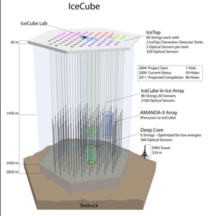
. IceCube is a 1 km

3

neutrino telescope

currently under construction at the South Pole.

The detector will consist of 5160 optical sensors

deployed at depths between 1450 m and 2450 m in

clear Antarctic ice evenly distributed over 86

strings. An air shower array covering a surface

area of 1 km

2

above the in-ice detector will meas-

ure cosmic ray air showers in the energy range

from 300 TeV to above 1 EeV. The detector is de-

signed to detect neutrinos of all flavors: ν

e

, ν

μ

and

ν

τ

. With 59 strings currently in operation, con-

struction is 67% complete. Based on data taken

to date, the observatory meets its design goals.

Selected results will be presented.

Keywords:

neutrinos, cosmic rays, neutrino as-

tronomy.

I. INTRODUCTION

IceCube is a large kilometer scale neutrino tele-

scope currently under construction at the South Pole.

With the ability to detect neutrinos of all flavors over

a wide energy range from about 100 GeV to beyond

10

9

GeV, IceCube is able to address fundamental

questions in both high energy astrophysics and neu-

trino physics. One of its main goals is the search for

sources of high energy astrophysical neutrinos which

provide important clues for understanding the origin

of high energy cosmic rays.

The interactions of ultra high energy cosmic rays

with radiation fields or matter either at the source or

in intergalactic space result in a neutrino flux due to

the decays of the produced secondary particles such

as pions, kaons and muons. The observed cosmic

ray flux sets the scale for the neutrino flux and leads

to the prediction of event rates requiring kilometer

scale detectors, see for example

1

. As primary candi-

dates for cosmic ray accelerators, AGNs and GRBs

are thus also the most promising astrophysical point

source candidates of high energy neutrinos. Galactic

source candidates include supernova remnants, mi-

croquasars, and pulsars. Guaranteed sources of neu-

trinos are the cosmogenic high energy neutrino flux

from interactions of cosmic rays with the cosmic mi-

crowave background and the galactic neutrino flux

resulting from galactic cosmic rays interacting with

the interstellar medium. Both fluxes are small and

their measurement constitutes a great challenge.

Other sources of neutrino radiation include dark mat-

ter, in the form of supersymmetric or more exotic

particles and remnants from various phase transitions

in the early universe.

The relation between the cosmic ray flux and the

atmospheric neutrino flux is well understood and is

based on the standard model of particle physics. The

observed diffuse neutrino flux in underground labo-

ratories agrees with Monte Carlo simulations of the

primary cosmic ray flux interacting with the Earth's

atmosphere and producing a secondary atmospheric

neutrino flux

2

.

Although atmospheric neutrinos are the primary

background in searching for astrophysical neutrinos,

they are very useful for two reasons. Atmospheric

neutrino physics can be studied up to PeV energies.

The measurement of more than 50,000 events per

year in an energy range from 500 GeV to 500 TeV

will make IceCube a unique instrument to make pre-

cise comparisons of atmospheric neutrinos with

model predictions. At energies beyond 100 TeV a

harder neutrino spectrum may emerge which would

be a signature of an extraterrestrial flux. Atmos-

pheric neutrinos also give the opportunity to cali-

brate the detector. The absence of such a calibration

beam at higher energies poses a difficult challenge

for detectors at energies targeting the cosmogenic

neutrino flux.

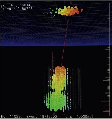
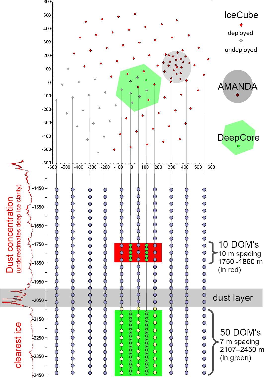
Fig. 1 Schematic view of IceCube. Fifty-nine of 86 strings are in

operation since 2009.

---

2

A. Karle et al., IceCube

II. DETECTOR AND CONSTRUCTION STA-

TUS

IceCube is designed to detect muons and cascades

over a wide energy range. The string spacing was

chosen in order to reliably detect and reconstruct

muons in the TeV energy range and to precisely

calibrate the detector using flashing LEDs and at-

mospheric muons.

The optical properties of the

South Pole Ice have been measured with various

calibration devices

3

and are used for modeling the

detector response to charged particles. Muon recon-

struction algorithms

4

allow measuring the direction

and energy of tracks from all directions.

In its final configuration, the detector will consist

of 86 strings reaching a depth of 2450 m below the

surface. There are 60 optical sensors mounted on

each string equally spaced between 1450m and

2450m depth with the exception of the six Deep

Core strings on which the sensors are more closely

spaced between 1760m and 2450m. In addition there

will be 320 sensors deployed in 160 IceTop tanks on

the surface of the ice directly above the strings. Each

sensor consists of a 25cm photomultiplier tube

(PMT), connected to a waveform recording data ac-

quisition circuit capable of resolving pulses with

nanosecond precision and having a dynamic range of

at least 250 photoelectrons per 10ns. With the most

recent construction season ending in February 2008,

half of the IceCube array has been deployed.

The detector is constructed by drilling holes in

the ice, one at a time, using a hot water drill. Drilling

is immediately followed by deployment of a detector

string into the water-filled hole. The drilling of a

hole to a depth of 2450m takes about 30 hours. The

subsequent deployment of the string typically takes

less than 10 hours. The holes typically freeze back

within 1-3 weeks. The time delay between two sub-

sequent drilling cycles and string deployments was

in some cases shorter than 50 hours. By the end of

February 2009, 59 strings and IceTop stations had

been deployed. We refer to this configuration as

IC59. Once the strings are completely frozen in the

commissioning can start. Approximately 99% of the

deployed DOMs have been successfully commis-

sioned. The 40-string detector configuration (IC40)

has been in operation from May 2008 to the end of

April 2009.

III. MUONS AND NEUTRINOS

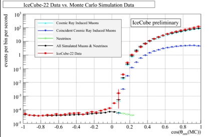
At the depth of IceCube, the event rate from

downgoing atmospheric muons is close to 6 orders

of magnitude higher than the event rate from atmos-

pheric neutrinos. Fig. 2 shows the observed muon

rate (IC22) as a function of the zenith angle

5

.

IceCube is effective in detecting downward going

muons.

A first measurement of the muon energy

spectrum is provided in the references

6

.

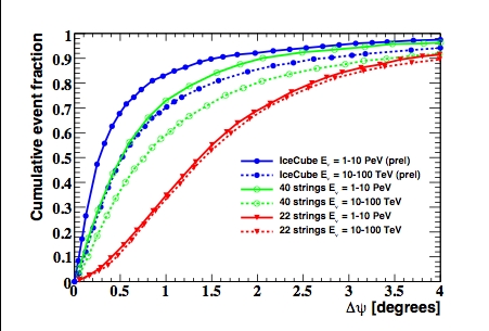
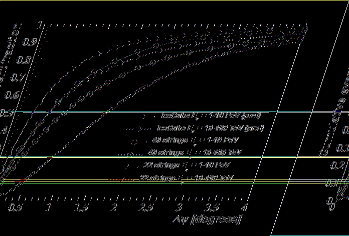
A good angular resolution of the experiment is the

basis for the zenith angle distribution and much more

so for the search of point sources of neutrinos from

galactice sources, AGNs or GRBs. Figure 3 shows

the angular resolution of IceCube for several detector

configurations based on high quality neutrino event

selections as used in the point source search for

IC40

7

.

The median angular resolution of IC40

achieved is already 0.7°, the design parameter for the

full IceCube.

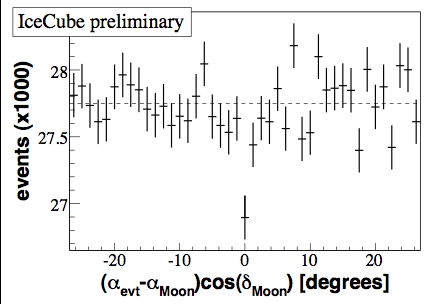
The muon flux serves in many ways also as a

calibration tool. One method to verify the angular

resolution and absolute pointing of the detector uses

the Moon shadow of cosmic rays.

The Moon

reaches an elevation of about 28° above the horizon

at the South Pole. Despite the small altitude of the

Moon, the event rate and angular resolution of

IceCube are sufficient to measure the cosmic ray

shadow of the Moon by mapping the muon rate in

the vicinity of the Moon. The parent air showers

have an energy of typically 30 TeV, well above the

energy where magnetic fields would pose a signifi-

Fig. 2 Muon rate in IceCube as a function of zenith angle

5

.The

data agree with the detector simulation which includes atmos-

pheric neutrinos, atmospheric muons, and coincident cosmic ray

muons (two muons erroneously reconstructed as a single track.)

Fig. 3 The angular resolution function of different IceCube con-

figurations is shown for two neutrino energy ranges samples from

an E

-2

energy spectrum.

---

PROCEEDINGS OF 31

st

ICRC, ŁÓDŹ 2009

3

cant deviation from the direction of the primary

particles. Fig. 4 shows a simple declination band

with bin size optimized for this analysis. A deficit of

~900 events (~4.2σ) is observed on a background of

~28000 events in 8 months of data taking. The defi-

cit is in agreement with expectations and confirms

the assumed angular resolution and absolute point-

ing.

The full IceCube will collect of order 50 000 high

quality atmospheric neutrinos per year in the TeV

energy range. A detailed understanding of the re-

sponse function of the detector at analysis level is the

foundation for any neutrino flux measurement. We

use the concept of the neutrino effective area to

describe the response function of the detector with

respect to neutrino flavor, energy and zenith angle.

The neutrino effective area is the equivalent area for

which all neutrinos of a given neutrino flux imping-

ing on the Earth would be observed. Absorption ef-

fects of the Earth are considered as part of the detec-

tor and folded in the effected area.

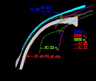
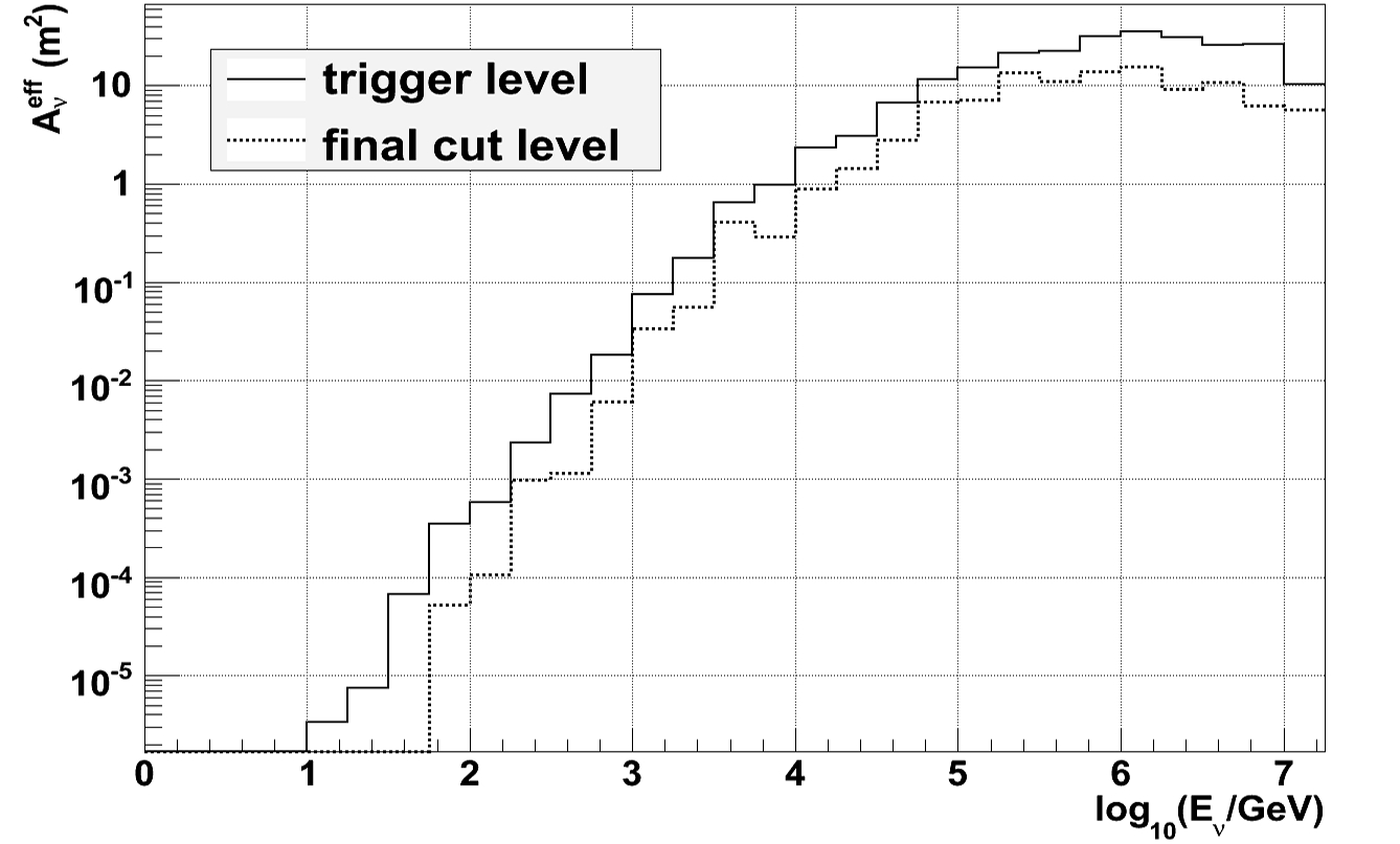
Figure 5 provides an overview of effective areas

for various analyses that are presented at this confer-

ence. First we note that the effective area increases

strongly in the range from 100 GeV to about 100

TeV. This is due to the increase in the neutrino-

nucleon cross-section and, in case of the muons, the

workhorse of high energy neutrino astronomy, due to

the additional increase of the muon range. Above

about 100 GeV, the increase slows down because of

radiative energy losses of muons.

The IC22

8

and IC80 as well as IC86 (IC80+6

Deep core) atmospheric ν

μ

area are shown for upgo-

ing neutrinos. The shaded area (IC22) indicates the

range from before to after quality cuts. The effective

area of IC40 point source analysis

7

is shown for all

zenith angles. It combines the upward neutrino sky

(predominantly energies < 1PeV) with downgoing

neutrinos (predominantly >1 PeV). Also shown is

the all sky ν

μ

+ ν

τ

area of IC80.

The ν

e

effective area is shown for the current

IC22 contained cascade analysis

9

as well as the IC22

extremely high energy (EHE) analysis

10

. It is inter-

esting to see how two entirely different analysis

techniques match up nicely at the energy transition

of about 5 PeV.

The cascade areas are about a factor of 20 smaller

than the ν

μ

areas, primarily because the muon range

allows the detection of neutrino interactions far out-

side the detector, increasing the effective detector

volume by a large factor. However, the excellent

energy resolution of contained cascades will benefit

the background rejection of any diffuse analysis, and

makes cascades a competitive detection channel in

the detector where the volume grows faster than the

area with the growing number of strings.

The figure illustrates why IceCube, and other

large water/ice neutrino telescopes for that matter,

can do physics over such a wide energy range. Un-

like typical air shower cosmic ray or gamma ray de-

tectors, the effective area increases by about 8 orders

of magnitude (10

-4

m

2

to 10

+4

m

2

) over an energy

range of equal change of scale (10 GeV to 10

9

GeV).

The analysis at the vastly different energy scales re-

Fig. 4 4.2σ deficit of events from direction of Moon in the

IceCube 40-string detector confirms pointing accuracy.

Fig. 6 The energy resolution for muons is approximately 0.3 in

log(energy) over a wide energy range

Fig. 5 The neutrino effective area is shown for a several IceCube

configurations (IC22, IC 40, IC86), neutrino flavors, energy

ranges and analysis levels (trigger, final analysis).

---

4

A. Karle et al., IceCube

quires very different approaches, which are pre-

sented in numerous talks in the parallel sessions

11, 45

.

The measurement of atmospheric neutrino flux

requires a good understanding of the energy re-

sponse. The energy resolution for muon neutrinos in

the IC22 configuration is shown in Fig. 6

8

. Over a

wide energy range (1 – 10000 TeV) the energy reso-

lution is ~0.3 in log(energy). This resolution is

largely dominated by the fluctuations of the muon

energy loss over the path length of 1 km or less.

IV. ATMOSPHERIC NEUTRINOS AND THE

SEARCH FOR ASTROPHYSICAL NEUTRINOS

We have discussed the effective areas, as well as

the angular and energy resolution of the detector.

Armed with these ingredients we can discuss some

highlights of neutrino measurements and astrophysi-

cal neutrino searches.

Figure 7 shows a preliminary measurement ob-

tained with the IC22 configuration. An unfolding

procedure has been applied to extract this neutrino

flux. Also shown is the atmospheric neutrino flux as

published previously based on 7 years of

AMANDA-II data. The gray shaded area indicates

the range of results obtained when applying the pro-

cedure to events that occurred primarily in the top or

bottom of the detector. The collaboration is devoting

significant efforts to understand and reduce system-

atic uncertainties as the statistics increases. The data

sample consists of 4492 high quality events with an

estimated purity of well above 95%. Several atmos-

pheric neutrino events are observed above 100 TeV,

pushing the diffuse astrophysical neutrino search

gradually towards the PeV energy region and higher

sensitivity. A look at the neutrino effective areas in

Fig. 5 shows that the full IceCube with 86 strings

will detect about one order of magnitude more

events: ~50000 neutrinos/year.

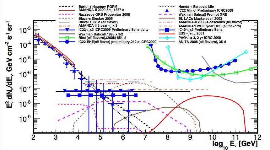
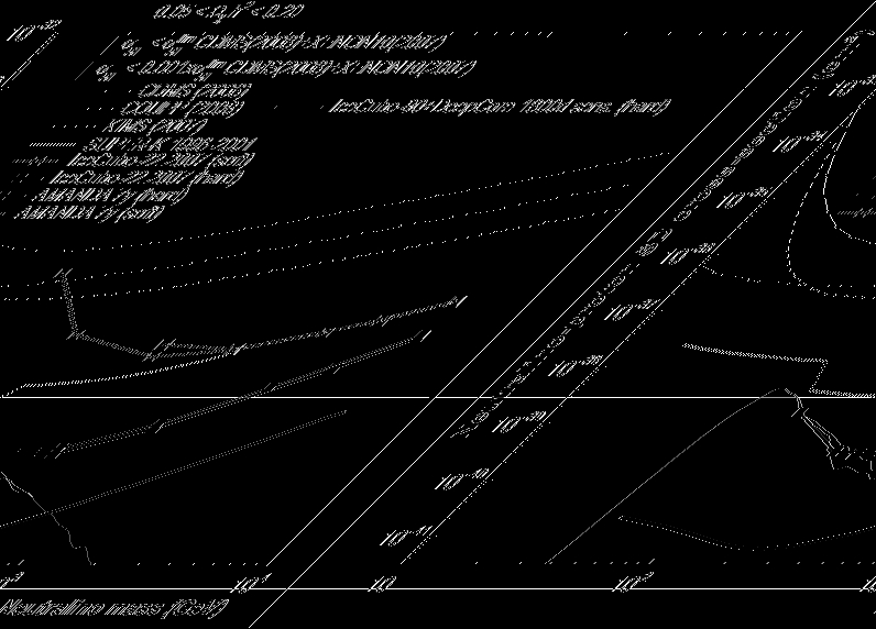
The search for astrophysical neutrinos is summa-

rized in Fig. 8. While the figure focuses on diffuse

fluxes, it is clear that some of these diffuse fluxes

may be detected as point sources. Some examples of

astrophysical flux models that are shown include

AGN Blazars

46

, BL Lacs

47

, Pre-cursor GRB models

and Waxman Bahcall bound

48

and Cosmogenic neu-

Fig. 7 Unfolded muon neutrino spectrum

8

averaged over zenith

angle, is compared to simulation and to the AMANDA result.

Data are taken with the 22 string configuration.

Fig. 8 Measured neutrino atmospheric neutrino fluxes from AMANDA and IceCube are shown together with a number of models for

astrophysical neutrinos and several limits by IceCube and other experiments

---

PROCEEDINGS OF 31

st

ICRC, ŁÓDŹ 2009

5

trinos

49

.

The following limits are shown for AMANDA

and IceCube:

• AMANDA-II, 2000-2006, atmospheric muon

neutrino flux

50

• IceCube-22 string, atmospheric neutrinos,

(preliminary)

8

• AMANDA-II, 2000-2003, diffuse E

-2

muon

neutrino flux limit

51

• AMANDA-II, 2000-2002, all flavors, not con-

tained events, PeV to EeV, E

-2

flux limit

52

• AMANDA-II, 2000-2004, cascades, contained

events, E

-2

flux limit

53

• IceCube-40, muon neutrinos, throughgoing

events, preliminary sensitivity

29

• IceCube-22, all flavor, throughgoing, downgo-

ing, extremely high energies (10 PeV to

EeV)

10

Also shown are a few experimental limits from

other experiments, including Lake Baikal

54

(diffuse,

not contained), and at higher energies some differen-

tial limits by RICE, Auger and at yet higher energies

energies from ANITA.

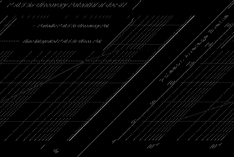
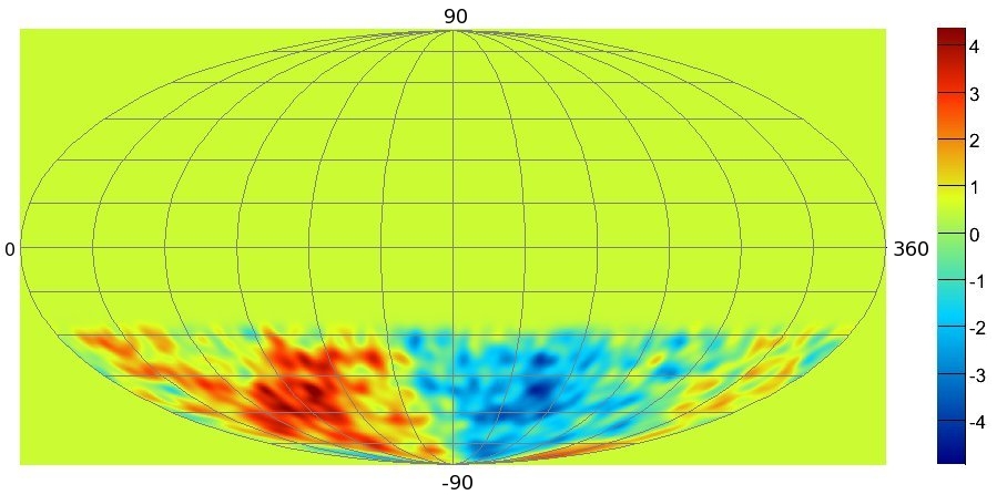
The skymap in Fig. 9 shows the probability for a

point source of high-energy neutrinos. The map was

obtained from 6 months of data taken with the 40

string configuration of IceCube. This is the first re-

sult obtained with half of IceCube instrumented.

The “hottest spot” in the map represents an excess of

7 events, which has a post-trial significance of 10

-4.4

.

After taking into account trial factors, the probability

for this event to happen anywhere in the sky map is

not significant. The background consists of 6796

neutrinos in the Northern hemisphere and 10,981

down-going muons rejected to the 10

-5

level in the

Southern hemisphere. The energy threshold for the

Southern hemisphere increases with increasing ele-

vation to reject the cosmic ray the muon background

by up to a factor of ~10

-5

. The energy of accepted

downgoing muons is typically above 100 TeV.

This unbinned analysis takes the angular resolu-

tion and energy information on an event-by-event

basis into account in the significance calculation.

The obtained sensitivity and discovery potential is

shown for all zenith angles in the figure.

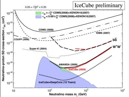
V. SEARCH FOR DARK MATTER

IceCube performs also searches for neutrinos pro-

duced by the annihilation of dark matter particles

gravitationally trapped at the center of the Sun and

the Earth. In searching for generic weakly interacting

massive dark matter particles (WIMPs) with spin-

independent interactions with ordinary matter,

IceCube is only competitive with direct detection

experiments if the WIMP mass is sufficiently large.

On the other hand, for WIMPs with mostly spin-

dependent interactions, IceCube has improved on the

previous best limits obtained by the SuperK experi-

ment using the same method. It improves on the best

limits from direct detection experiments by two or-

ders of magnitude. The IceCube limit as well as a

limit obtained with 7 years of AMANDA are shown

in the figure. It rules out supersymmetric WIMP

models not excluded by other experiments. The in-

stallation of the Deep Core of 6 strings as shown in

Fig. 1 will greatly enhance the sensitivity of IceCube

for dark matter. The projected sensitivity in the

range from 50 GeV to TeV energies is shown in Fig.

11. The Deep Core is an integral part of IceCube

and relies on the more closely spaced nearby strings

for the detection of low energy events as well as on a

highly efficient veto capability against cosmic ray

muon backgrounds using the surrounding IceCube

strings.

Fig, 9: The map shows the probability for a point source of high-

energy neutrinos on the atmospheric neutrino background. The

map was obtained by operating IceCube with 40 strings for half a

year

7

. The “hottest spot” in the map represents an excess of 7

events. After taking into account trial factors, the probability for

this event to happen anywhere in the sky map is not significant.

The background consists of 6796 neutrinos in the Northern hemi-

sphere and 10,981 down-going muons rejected to the 10

-5

level in

the Southern hemisphere.

Fig. 10 Upper limits to E

-2

-type astrophysical muon neutrino spec-

tra are shown for the newest result of ½ year of IC40 and a num-

ber of earlier results obtained by IceCube and other experiments.

---

6

A. Karle et al., IceCube

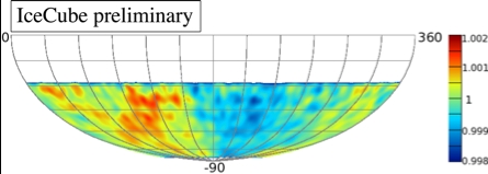
VI. COSMIC RAY MUONS AND HIGH ENERGY

COSMIC RAYS

IceCube is a huge cosmic-ray muon detector and

the first sizeable detector covering the Southern

hemisphere. We are using samples of several billion

downward-going muons to study the enigmatic large

and small scale anisotropies recently identified in the

cosmic ray spectrum by Northern detectors, namely

the Tibet array

55

and the Milagro array

56

. Fig. 12

shows the relative deviations of up to 0.001 from the

average of the Southern muon sky observed with the

22-string array

11

. A total of 4.3 billion events with a

median energy of 14 TeV were used. IceCube data

shows that these anisotropies persist at energies in

excess of 100 TeV ruling out the sun as their origin.

Having extended the measurement to the Southern

hemisphere should help to decipher the origin of

these unanticipated phenomena.

IceCube can detect events with energies ranging

from 0.1 TeV to beyond 1 EeV, neutrinos and cos-

mic ray muons.

The surface detector IceTop consists of ice Cher-

enkov tank pairs. Each IceTop station is associated

with an IceCube string. With a station spacing of

125 m, it is efficient for air showers above energies

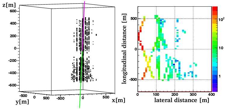
of 1 PeV. Figure 13 shows an event display of a

very high-energy (~EeV) air shower event. Hits are

recorded in all surface detector stations and a large

number of DOMs in the deep ice. Based on a pre-

liminary analysis some 2000 high-energy muons

would have reached the deep detector in this event if

the primary was a proton and more if it was a nu-

cleus. With 1 km

2

surface area, IceTop will acquire

a sufficient number of events in coincidence with the

in-ice detector to allow for cosmic ray measurements

up to 1 EeV. The directional and calorimetric meas-

urement of the high energy muon component with

the in-ice detector and the simultaneous measure-

ment of the electromagnetic particles at the surface

with IceTop will enable the investigation of the en-

ergy spectrum and the mass composition of cosmic

rays.

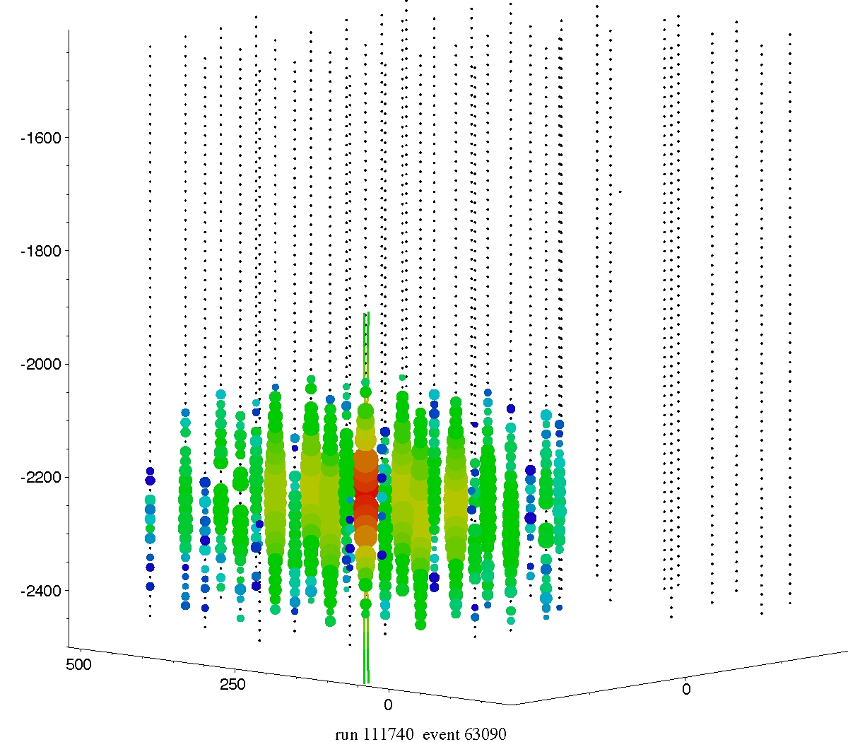
Events with energies above one PeV can deposit

an enormous amount of light in the detector. Figure

14 shows an event that was generated by flasher

pulse produced by an array of 12 UV LEDs that are

mounted on every IceCube sensor. The event pro-

duces an amount of light that is comparable with that

of an electron cascade on the order of 1 PeV. Pho-

tons were recorded on strings at distances up to 600

m from the flasher. The events are somewhat

brighter than previously expected because the deep

ice below a depth of 2100m is exceptionally clear.

Fig. 13 A very high energy cosmic ray air shower ob-

served both with the surface detector IceTop and the in-

ice detector string array.

Fig. 11 The red boxes show the upper limits at 90% confi-

dence level on the spin-dependent interaction of dark matter

particles with ordinary matter

18, 20

. The two lines represent the

extreme cases where the neutrinos originate mostly from

heavy quarks (top line) and weak bosons (bottom line) pro-

duced in the annihilation of the dark matter particles. Also

shown is the reach of the complete IceCube and its DeepCore

extension after 5 years of observation of the sun. The shaded

area represents supersymmetric models not disfavored by di-

rect searches for dark matter. Also shown are previous limits

from direct experiments and from the Superkamiokande ex-

periment.

Fig.12 The plot shows the skymap of the relative intensity in

the arrival directions of 4.3 billion muons produced by cosmic

ray interactions with the atmosphere with a median energy of

14 TeV; these events were reconstructed with an average angu-

lar resolution of 3 degrees. The skymap is displayed in equa-

torial coordinates.

---

PROCEEDINGS OF 31

st

ICRC, ŁÓDŹ 2009

7

The scattering length is substantially larger than in

average ice at the depth of AMANDA.

Extremely high energy (EHE) events, above about

1 PeV, are observed near and above the horizon. At

these energies, the Earth becomes opaque to neutri-

nos and one needs to change the search strategy. In

an optimized analysis, the neutrino effective area

reaches about 4000m

2

for IC80 at 1 EeV. IC80 can

therefore test optimistic models of the cosmogenic

neutrino flux. IceCube is already accumulating an

exposure with the current data that makes detection

of a cosmogenic neutrino event possible.

IceCube construction is on schedule to completion

in February 2011. The operation of the detector sta-

ble and data analysis of recent data allows a rapid in-

crease of the sensitivity and the discovery potential

of IceCube.

VII. ACKNOWLEDGEMENTS

We acknowledge the support from the following

agencies: U.S. National Science Foundation-Office

of Polar Program, U.S. National Science Foundation-

Physics Division, University of Wisconsin Alumni

Research Foundation, U.S. Department of Energy,

and National Energy Research Scientific Computing

Center, the Louisiana Optical Network Initiative

(LONI) grid computing resources; Swedish Research

Council, Swedish Polar Research Secretariat, and

Knut and Alice Wallenberg Foundation, Sweden;

German Ministry for Education and Research

(BMBF), Deutsche Forschungsgemeinschaft (DFG),

Germany; Fund for Scientific Research (FNRS-

FWO), Flanders Institute to encourage scientific and

technological research in industry (IWT), Belgian

Federal Science Policy Office (Belspo); the Nether-

lands Organisation for Scientific Research (NWO);

M. Ribordy acknowledges the support of the SNF

(Switzerland); A. Kappes and A. Groß acknowledge

support by the EU Marie Curie OIF Program.

REFERENCES

[1] E. Waxman and J. Bahcall, Phys. Rev. D 59 (1998)

023002

[2] T. Gaisser,

Cosmic Rays and Particle Physics

Cambridge University Press 1991

[3] M.Ackermann et al., J. Geophys. Res.

111

, D13203

(2006)

[4] J.Ahrens et al., Nucl. Inst. Meth. A

524

, 169 (2004)

[5] P.
Berghaus
for
the
IceCube

Collaboration,

proc.


Proc.
for
the
XV
International
Symposium
on
Very


High
Energy
Cosmic
Ray
Interactions
(ISVHECRI


2008),
Paris,
France,
arXiv:0902.0021

[6] P. Berghaus

et al.

, Direct Atmospheric Muon Energy

Spectrum Measurement with IceCube (IceCube col-

laboration), Proc. of the 31

st

ICRC HE1.5; astro-

ph.HE/arXiv: 0909.0679

[7] J. Dumm

et al.

, Likelihood Point-Source Search with

IceCube (IceCube collaboration), Proc. of the 31

st

ICRC OG2.5D.

[8] D. Chirkin

et al.

, Measurement of the Atmospheric

Neutrino Energy Spectrum with IceCube (IceCube

collaboration), Proc. of the 31

st

ICRC HE2.2

[9] J. Kiryluk

et al.

, First Search for Extraterrestrial Neu-

trino-Induced Cascades with IceCube (IceCube col-

laboration), Proc. of the 31

st

ICRC OG2.5; astro-

ph.HE/arXiv: 0909.0989

[10] K. Mase

et al.

, The Extremely High-Energy Neutrino

Search with IceCube (IceCube collaboration), Proc. of

the 31

st

ICRC HE1.4

[11] R. Abbasi and P. Desiati, JC Díaz Vélez

et al.

, Large-

Scale Cosmic-Ray Anisotropy with IceCube (IceCube

collaboration), Proc. of the 31

st

ICRC SH3.2; astro-

ph.HE/0907.0498

[12] K. Andeen

et al.

, Composition in the Knee Region

with SPASE-AMANDA (IceCube collaboration),

Proc. of the 31

st

ICRC HE1.2

[13] C. Rott et al., Atmospheric Neutrino Oscilaton

Measurement with IceCube (IceCube collaboration),

Proc. of the 31

st

ICRC HE2.3

[14] M. Baker

et al.

, IceCube Time-Dependent Point-

Source Analysis Using Multiwavelength Information

(IceCube collaboration), Proc. of the 31

st

ICRC OG2.5

[15] J. Bazo Alba

et al.

, Search for Neutrino Flares from

Point Sources with IceCube (IceCube collaboration,

to

appear in

Proc. of the 31

st

ICRC OG2.5

[16] M. Bissok

et al.,

Sensor Development and Calibration

for Acoustic Neutrino Detection in Ice (IceCube col-

laboration), Proc. of the 31

st

International Cosmic Ray

Conference, Lodz, Poland (2009) HE2.4; astro-

ph.IM/09073561

[17] D. Boersma

et al.

, Moon-Shadow Observation by

IceCube (IceCube collaboration), Proc. of the 31

st

ICRC OG2.5

Figure 14: A flasher event in IceCube. Such events,

produced by LEDs built in the DOMs, can be used for

calibration purposes.

---

8

A. Karle et al., IceCube

[18] J. Braun and D. Hubert

et al.

, Searches for WIMP

Dark Matter from the Sun with AMANDA (IceCube

collaboration), Proc. of the 31

st

ICRC HE2.3; astro-

ph.HE/09061615

[19] M. D’Agostino

et al.

, Search for Atmospheric Neu-

trino-Induced Cascades (IceCube collaboration), Proc.

of the 31

st

ICRC HE2.2; ; astro-

ph.HE/arXiv:0910.0215

[20] M. Danninger and K. Han

et al.

, Search for the Ka-

luza-Klein Dark Matter with the AMANDA/IceCube

Detectors (IceCube collaboration), Proc. of the 31

st

ICRC HE2.3; astro-ph.HE/0906.3969

[21] F. Descamps

et al.

, Acoustic Detection of High-

Energy Neutrinos in Ice (IceCube collaboration), Proc.

of the 31

st

ICRC HE2.4

[22] M. Duvoort

et al.

, Search for GRB Neutrinos via a

(Stacked) Time Profile Analysis (IceCube collabor-

ation), Proc. of the 31

st

ICRC OG2.4

[23] S. Euler

et al.

, Implementation of an Active Veto

against Atmospheric Muons in IceCube DeepCore

(IceCube collaboration), Proc. of the 31

st

ICRC OG2.5

[24] T. Feusels

et al.

, Reconstruction of IceCube Coinci-

dent Events and Study of Composition-Sensitive Ob-

servables Using Both the Surface and Deep Detector

(IceCube collaboration), Proc. of the 31

st

ICRC HE1.3

[25] A. Francowiak

et al.

, Optical Follow-Up of High-

Energy Neutrinos Detected by IceCube (IceCube and

ROTSE collaborations), Proc. of the 31

st

ICRC OG2.5

[26] R. Franke

et al.

, Neutrino Triggered High-Energy

Gamma-Ray Follow-Up with IceCube (IceCube col-

laboration), Proc. of the 31

st

ICRC OG2.5

[27] L. Gerhardt

et al.

, Study of High p_T Muons in

IceCube (IceCube collaboration), Proc. of the 31

st

ICRC HE1.5; astro-ph.HE/arXiv 0909.0055

[28] D. Grant

et al.

, Fundamental Neutrino Measurements

with IceCube DeepCore (IceCube collaboration),

Proc. of the 31

st

ICRC HE2.2

[29] K. Hoshina

et al.

, Search for Diffuse High-Energy

Neutrinos with IceCube (IceCube collaboration), Proc.

of the 31

st

ICRC OG2.5

[30] W. Huelsnitz

et al.,

Search for Quantum Gravity with

IceCube and High-Energy Atmospheric Neutrinos

(IceCube collaboration), Proc. of the 31

st

ICRC HE2.3

[31] A. Ishihara

et al.

, Energy-Scale Calibration Using

Cosmic-Ray Induced Muon Bundles Measured by the

IceCube Detector with IceTop Coincident Signals

(IceCube collaboration), Proc. of the 31

st

ICRC HE1.5

[32] A. Kappes

et al.

, Searches for Neutrinos from GRBs

with the IceCube 22-String Detector and Sensitivity

Estimates for the Full Detector (IceCube collabor-

ation), Proc. of the 31

st

ICRC OG2.4

[33] F. Kislat

et al.

, A First All-Particle Cosmic-Ray En-

ergy Spectrum from IceTop (IceCube collaboration),

Proc. of the 31

st

ICRC HE1.2

[34] M. Kowarik

et al.

, Supernova Search with the

AMANDA / IceCube Neutrino Telescopes (IceCube

collaboration), Proc. of the 31

st

ICRC OG2.2

[35] D. Lennarz

et al.

, Search for High-Energetic Neutrinos

from Supernova Explosions with AMANDA (IceCube

collaboration), Proc. of the 31

st

ICRC OG2.5; astro-

ph.HE/09074621

[36] K. Meagher

et al.

, Search for Neutrinos from GRBs

with IceCube (IceCube collaboration), Proc. of the 31

st

ICRC OG2.4

[37] E. Middell

et al.

, Improved Reconstruction of Cas-

cade-Like Events (IceCube collaboration), Proc. of the

31

st

ICRC OG2.5

[38] C. Portello-Roucelle

et al.

, IceCube / AMANDA

Combined Analyses for the Search of Neutrino Sour-

ces at Low Energies (IceCube collaboration), Proc. of

the 31

st

ICRC OG2.5

[39] C. Rott

et al.

, Results and Prospects of Indirect

Searches fo Dark Matter with IceCube (IceCube col-

laboration), Proc. of the 31

st

ICRC HE2.3

[40] B. Ruzybayev

et al.

, Small Air Showers in IceCube

(IceCube collaboration), Proc. of the 31

st

ICRC HE1.1

[41] A. Schukraft and J. Hülß

et al.

, AMANDA 7-Year

Multipole Analysis (IceCube collaboration), Proc. of

the 31

st

ICRC OG2.5; astro-ph.HE/09063942

[42] S. Seo

et al.

, Search for High-Energy Tau Neutrinos in

IceCube (IceCube collaboration), Proc. of the 31

st

ICRC OG2.5

[43]

43

A. Silvestri

et al.

, Search for Ultra–High-Energy

Neutrinos with AMANDA (IceCube collaboration),

Proc. of the 31

st

ICRC OG2.5

[44] S. Tilav

et al.

, Atmospheric Variations as Observed by

IceCube (IceCube collaboration), Proc. of the 31

st

ICRC HE1.1

[45] C. Wiebusch

et al.

, Physics Capabilities of the

IceCube DeepCore Detector (IceCube collaboration),

Proc. of the 31

st

ICRC OG2.5; astro-ph.IM/09072263

[46] F. W. Stecker. Phys. Rev. D, 72(10):107301, 2005

[47] A. Mücke et al. Astropart. Phys., 18:593, 2003

[48] S. Razzaque, P. Meszaros, and E. Waxman. Phys.

Rev. D, 68(8):083001, 2003

[49] R. Engel, D. Seckel, and T. Stanev. Phys. Rev. D,

64(9):093010, 2001

[50] A. Achterberg

et al

. (IceCube collaboration),

Phys.Rev.D

79

102005, 2009

[51] A. Achterberg

et al

. (IceCube collaboration),, Phys.

Rev. D

76

042008 (2007);

[52] Ackerman

et al

. (IceCube collaboration), Astrophys.

Jour.

675

2 1014-1024 (2008); astro-ph/07113022

[53] A. Achterberg,

et al

., Astrophys. Jour.

664

397-410

(2007); astro-ph/0702265v2

[54] A.V.Avrorin

et al.

, Astronomy Letters, Vol.35, No.10,

pp.651-662, 2009; arXiv:0909.5562

[55] M. Amenomori et al. [The Tibet AS-Gamma

Collaboration], Astrophys. J. 633, 1005 (2005)

arXiv:astroph/0502039

[56] A.A. Abdo et al., Phys. Rev. Lett. 101: 221101

(2008), arXiv:0801.3827

---

PROCEEDINGS OF THE 31

st

ICRC, ŁOD´ Z´ 2009

1

All-Sky Point-Source Search with 40 Strings of IceCube

Jon Dumm

∗

, Juan A. Aguilar

∗

, Mike Baker

∗

, Chad Finley

∗

, Teresa Montaruli

∗

,

for the IceCube Collaboration

†

∗

Dept. of Physics, University of Wisconsin, Madison, WI, 53706, USA

†

See the special section of these proceedings.

Abstract. During 2008-09, the IceCube Neutrino

Observatory was operational with 40 strings of

optical modules deployed in the ice. We describe

the search for neutrino point sources based on a

maximum likelihood analysis of the data collected

in this configuration. This data sample provides the

best sensitivity to high energy neutrino point sources

to date. The field of view is extended into the down-

going region providing sensitivity over the entire

sky. The 22-string result is discussed, along with

improvements leading to updated angular resolution,

effective area, and sensitivity. The improvement in

the performance as the number of strings is increased

is also shown.

Keywords: neutrino astronomy

I. INTRODUCTION

The primary goal of the IceCube Neutrino Obser-

vatory is the detection of high energy astrophysical

neutrinos. Such an observation could reveal the origins

of cosmic rays and offer insight into some of the

most energetic phenomena in the Universe. In order to

detect these neutrinos, IceCube will instrument a cubic

kilometer of the clear Antarctic ice sheet underneath the

geographic South Pole with an array of 5,160 Digital

Optical Modules (DOMs) deployed on 86 strings from

1.5–2.5 km deep. This includes six strings with a smaller

DOM spacing and higher quantum efficiency compris-

ing DeepCore, increasing the sensitivity to low energy

neutrinos <∼ 100 GeV. IceCube also includes a surface

array (IceTop) for observing extensive air showers of

cosmic rays. Construction began in the austral sum-

mer 2004–05, and is planned to finish in 2011. Each

DOM consists of a 25 cm diameter Hamamatsu photo-

multiplier tube, electronics for waveform digitization,

and a spherical, pressure-resistant glass housing. The

DOMs detect Cherenkov photons induced by relativistic

charged particles passing through the ice. In particular,

the directions of muons (either from cosmic ray showers

above the surface, or neutrino interactions within the ice

or bedrock) can be well reconstructed from the track-like

pattern and timing of hit DOMs.

The 22-string results presented in the discussion are

from a traditional up-going search. In such a search,

neutrino telescopes use the Earth as a filter for the large

background of atmospheric muons, leaving only an irre-

ducible background of atmospheric neutrinos below the

horizon. These have a softer spectrum (∼ E

−3.6

above

100 GeV) than astrophysical neutrinos which originate

from the decays of particles accelerated by the first order

Fermi mechanism and thus are expected to have an E

−2

spectrum. This search extends the field of view above

the horizon into the large background of atmospheric

muons. In order to reduce this background, strict cuts on

the energy of events need to be applied. This makes the

search above the horizon primarily sensitive to extremely

high energy (> PeV) sources.

II. METHODOLOGY

An unbinned maximum likelihood analysis, account-

ing for individual reconstructed event uncertainties and

energy estimators, is used in IceCube point source anal-

yses. A full description can be found in Braun et al. [1].

This method improves the sensitivity to astrophysical

sources over directional clustering alone by leveraging

the event energies in order to separate hard spectrum

signals from the softer spectrum of the atmospheric

neutrino or muon background. For each tested direction

in the sky, the best fit is found for the number of signal

events n

s

over background and the spectral index of

a power law γ of the excess events. The likelihood

ratio of the best-fit hypothesis to the null hypothesis

(n

s

= 0) forms the test statistic. The significance of

the result is evaluated by performing the analysis on

scrambled data sets, randomizing the events in right

ascension but keeping all other event properties fixed.

Uniform exposure in right ascension is ensured as the

detector rotates completely each day, and the location

at 90

◦

south latitude gives a uniform background for

each declination band. Events that are nearly vertical

(declination < −85

◦

or > 85

◦

) are left out of the

analysis, since scrambling in right ascension does not

work in the polar regions.

Two point-source searches are performed. The first is

an all-sky search where the maximum likelihood ratio

is evaluated for each direction in the sky on a grid,

much finer than the angular resolution. The significance

of any point on the grid is determined by the fraction

of scrambled data sets containing at least one grid point

with a log likelihood ratio higher than the one observed

in the data. This fraction is the post-trial p-value for

the all-sky search. Because the all-sky search includes

a large number of effective trials, the second search is

restricted to the directions of a priori selected sources

of interest. The post-trial p-value for this search is again

---

2

J. DUMM et al. ICECUBE POINT SOURCE ANALYSIS

calculated by performing the same analysis on scrambled

data sets.

III. EVENT SELECTION

Forty strings of IceCube were operational from April

2008 to May 2009 with ∼ 90% duty cycle after a good

run selection based on detector stability. The ∼ 3× 10

10

triggered events per year are first reduced to ∼ 1 × 10

9

events using low-level likelihood reconstructions and

energy estimators as part of an online filtering system

on site. These filtered events are sent over satellite to a

data center in the North for further processing, including

higher-level likelihood reconstructions for better angular

resolution. Applying the analysis-level cuts (described

below) that optimize the sensitivity to point sources

finally yields a sample of ∼ 3 × 10

4

events. Due to

offline filtering constraints, 144 days of livetime were

used to design the analysis strategy and finalize event

selection, keeping the time and right ascension of the

events blinded. This represents about one-half of the

final 40-string data sample. Because the northern sky

and southern sky present very different challenges, two

techniques are used to reduce the background due to

cosmic ray muons.

For the northern sky, the Earth filters out atmospheric

muons. Only neutrinos can penetrate all the way through

the Earth and interact near the detector to create up-

going muons. However, since down-going atmospheric

muons trigger the detector at ∼ 1 kHz, even a small

fraction of mis-reconstructed events contaminates the

northern sky search. Events may be mis-reconstructed

due to random noise or light from muons from indepen-

dent cosmic ray showers coincident in the same readout

window of ± 10 µs. Therefore, strict event selection

is still required to reject mis-reconstructed down-going

events. This selection is based on track-like quality

parameters (the reduced likelihood of the track fit and

the directional width of the likelihood space around

the best track fit [2]), a likelihood ratio between the

best up-going and down-going track solution, and a

requirement that the event’s set of hits can be split

into two parts which both reconstruct as nearly-upgoing.

Although the track-like quality parameters have very

little declination dependence, these last two parameters

only work for selecting up-going neutrino candidates

and remove down-going events. This event selection

provides an optimal sensitivity to sources of neutrinos

in the TeV–PeV energy range.

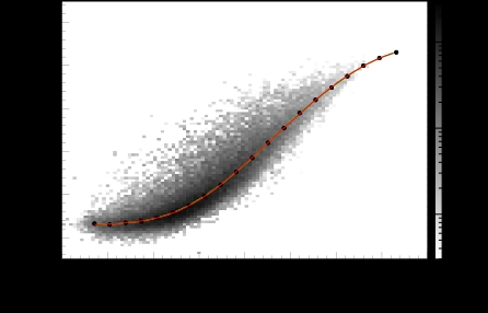
In the southern sky, energy estimators were used to

separate the large number of atmospheric muons from a

hypothetical source of neutrinos with a harder spectrum.

After track-quality selections, similar but tighter than

for the up-going sample, a cut based on an energy

estimator is made until a fixed number of events per

steradian is achieved. Because only the highest energy

events pass the selection, sensitivity is primarily to

neutrino sources at PeV energies and above. Unlike

for the northern sky, which is a ∼ 90% pure sample

ν

/ GeV )

10

(E

log

2

3

4

5

6

7

8

9

(E/GeV)]

10

dP/d[log

0

0.1

0.2

0.3

0.4

0.5

0.6

0.7

0.8

Atmospheric (up-going)

-2

(up-going)

E

-2

(down-going)

E

-1.5

(down-going)

E

Fig. 1: Probability density (P) of neutrino energies at

final cut level for atmospheric and an E

−2

spectrum of

neutrinos averaged over the northern sky and E

−1.5

in

the southern sky.

of neutrino-induced muons, the event sample in the

southern sky is almost entirely well-reconstructed high

energy atmospheric muons and muon bundles.

IV. PERFORMANCE

The performance of the detector and the analysis

is characterized using a simulation of ν

µ

and ν¯

µ

. At-

mospheric muon background is simulated using COR-

SIKA [3]. Muon propagation through the Earth and

ice are done using MMC [4]. A detailed simulation of

the ice [5] propagates the Cherenkov photon signal to

each DOM. Finally, a simulation of the DOM, including

angular acceptance and electronics, yields an output

treated identically to data. For an E

−2

spectrum of

neutrinos the median angular difference between the

neutrino and the reconstructed direction of the muon in

the northern (southern) sky is 0.8

◦

(0.6

◦

). The different

energy distributions in each hemisphere shown in Fig. 1

cause this effect, since the reconstruction performs better

at higher energies. The cumulative point spread functions

for the 22-, 40-, and 80-string configurations of IceCube

are shown in Fig. 2 for two different ranges of energy.

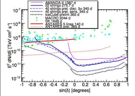
Fig. 3 shows the effective area to an equal-ratio flux

of ν

µ

+ ν¯

µ

. Fig. 4 shows the 40-string sensitivity to

an E

−2

spectrum of neutrinos for 330 days of livetime

and compared to the 22-string configuration of IceCube,

as well as ANTARES sensitivity, primarily relevant for

the southern sky. The 80-string result uses the same

methodology and event selection for the up-going region

as this work.

V. DISCUSSION

The previous season of IceCube data recorded with

the 22-string configuration has already been the subject

of point source searches [7]. The analysis included

5114 atmospheric neutrino events including a contam-

ination of about 5% of atmospheric muons during a

livetime of about 276 days. No evidence was found

for a signal, and the largest significance is located at

---

PROCEEDINGS OF THE 31

st

ICRC, ŁOD´ Z´ 2009

3

Fig. 2: The point spread function of the 22-, 40-, and 80-

string IceCube configurations in two energy bins. This

is the cumulative distribution of the angular difference

between the neutrino and recostructed muon track using

simulated neutrinos. The large improvement between the

22- and 40-string point spread function at high energies

is due to an improvement in the reconstruction, which

now uses charge information.

ν

/ GeV )

10

( E

log

2

3

4

5

6

7

8

9

]

2

Effective Area [m

μ

ν

+

μ

ν

-3

10

-2

10

-1

10

1

10

2

10

3

10

4

10

zenith range (0

°

, 30

°

)

zenith range (30

°

, 60

°

)

zenith range (60

°

, 90

°

)

zenith range (90

°

, 120

°

)

zenith range (120

°

, 150

°

)

zenith range (150

°

, 180

°

)

Fig. 3: The IceCube 40-string solid-angle-averaged ef-

fective area to an equal-ratio flux of ν

µ

and ν¯

µ

, recon-

structed within 2

◦

of the true direction. The different

shapes of each zenith band are due to a combination of

event selection and how much of the Earth the neutrinos

must travel through. Since the chance of a neutrino

interacting increases with its energy, in the very up-going

region high energy neutrinos are absorbed in the Earth.

Only near the horizon do muons from > PeV neutrinos

often reach IceCube. Above the horizon, low energy

events are removed by cuts, and in the very down-going

region effective area for high energies is lost due to

insufficient target material.

153.4

◦

r.a., 11.4

◦

dec. Accounting for all trial factors,

this is consistent with the null hypothesis at the 2.2 σ

level. The events in the most significant location did

not show a clear time dependent pattern, and these

coordinates have been included in the catalogue of

sources for the 40-string analysis.

Declination [degrees]

-80 -60 -40 -20

0

20

40

60

80

]

-1

s

-2

dN/dE [TeV cm

2

E

-12

10

-11

10

-10

10

-9

10

22 strings 275.7 d

40 strings prel. sens. 330 d

IceCube prelim 365 d

ANTARES prel. 365 d

Fig. 4: 40-string IceCube sensitivity for 330 days as

a function of declination to a point source with dif-

ferential flux

dΦ

dE

= Φ

0

(E/TeV)

−2

. Specifically, Φ

0

is

the minimum source flux normalization (assuming E

−2

spectrum) such that 90% of simulated trials result in a

log likelihood ratio log λ greater than the median log

likelihood ratio in background-only trials (log λ = 0).

Comparison are also shown for the 22-string and the

expected performance of the 80-string configuration, as

well as the ANTARES [6] sensitivity.

Since the 22-string analysis, a number of improve-

ments have been achieved. An additional analysis of

the 22-string data optimized for E

−2

and harder spectra

was performed down to −50

◦

declination with a binned

search [8]. These analyses are now unified into one

all-sky search which uses the energy of the events and

extends to −85

◦

declination. Secondly, a new recon-

struction that uses the charge observed in each DOM

performs better, especially on high energy events. Third,

an improved energy estimator, based on the photon

density along the muon track, has a better muon energy

resolution.

With construction more than half-complete, IceCube

is already beginning to demonstrate its potential as an

extraterrestrial neutrino observatory. The latest science

run with 40 strings was the first detector configuration

with one axis the same length as that of the final array.

Horizontal muon tracks reconstructed along this axis

provide the first class of events of the same quality as

those in the finished 80-string detector.

There are now 59 strings of IceCube deployed and

taking data. Further development of reconstruction and

analysis techniques, through a better understanding of

the detector and the depth-dependent properties of the

ice, have continued to lead to improvements in physics

results. New techniques in the southern sky may include

separating muon bundles of cosmic ray showers from

single muons induced by high energy neutrinos. At lower

energies, the identification of starting muon tracks from

neutrinos interacting inside the detector will be helped

with the addition of DeepCore [9].

---

4

J. DUMM et al. ICECUBE POINT SOURCE ANALYSIS

REFERENCES

[1] J. Braun et al. Methods for point source analysis in high energy

neutrino telescopes. Astropart. Phys. 29, 155, 2006.

[2] Neunhoffer, T. Astropart. Phys., 25, 220. 2006.

[3] D. Heck et al. CORSIKA: A Monte Carlo code to simulate

extensive air showers, FZKA, Tech. Rep., 1998.

[4] D. Chirkin and W. Rhode. Preprint hep-ph/0407075, 2004.

[5] J. Lundberg et al. Nucl. Inst. Meth., vol. A581, p. 619, 2007.

[6] J. A. Aguilar et al. Expected discovery potential and sensitivity to

neutrino point-like sources of the ANTARES neutrino telescope.

in proceedings 30

th

ICRC, Merida. 2007.

[7] R. Abbasi et al. (IceCube Collaboration) First Neutrino Point-

Source Results from IceCube in the 22-String Configuration.

submitted, 2009. astro-ph/09052253

[8] R. Lauer, E. Bernardini. Extended Search for Point Sources of

Neutrinos Below and Above the Horizon. in proceedings of 2

nd

Heidelberg Workshop, 2009, astro-ph/09035434.

[9] C. Wiebusch et al. (IceCube Collaboration), these proceedings.

---

PROCEEDINGS OF THE 31

st

ICRC, ŁO´ DZ´ 2009

1

IceCube Time-Dependent Point Source Analysis Using

Multiwavelength Information

M. Baker

∗

, J. A. Aguilar

∗

, J. Braun

∗

, J. Dumm

∗

, C. Finley

∗

, T. Montaruli

∗

, S. Odrowski

†

, E. Resconi

†

for the IceCube Collaboration

‡

∗

Dept. of Physics, University of Wisconsin, Madison, WI 53706, USA

†

Max-Planck-Institut fur Kernphysik, D-69177 Heidelberg, Germany

‡

see special section of these proceedings

Abstract

. In order to enhance the IceCube’s sen-

sitivity to astrophysical objects, we have developed

a dedicated search for neutrinos in coincidence

with flares detected in various photon wavebands

from blazars and high-energy binary systems. The

analysis is based on a maximum likelihood method

including the reconstructed position, the estimated

energy and arrival time of IceCube events. After a

short summary of the phenomenological arguments

motivating this approach, we present results from

data collected with 22 IceCube strings in 2007-2008.

First results for the 40-string IceCube configuration

during 2008-2009 will be presented at the conference.

We also report on plans to use long light curves and

extract from them a time variable probability density

function.

Keywords

: Neutrino astronomy, Multiwavelength

astronomy

I. INTRODUCTION

IceCube is a high-energy neutrino observatory cur-

rently under construction at the geographic South Pole.

The full detector will be composed of 86 strings of

60 Digital Optical Modules (DOMs) each, deployed

between 1500 and 2500m below the glacier surface. A

six string Deep Core with higher quantum efficiency

photomultipliers and closer DOM spacing in the lower

detector will enhance sensitivity to low energy neutrinos.

Muons passing through the detector emit Cˇ erenkov light

allowing reconstruction with

? 1

◦

angular resolution

in the full detector and about

1.5

◦

(median) in the

22 string configuration. In this paper we describe the

introduction of a time dependent term to the standard

search for steady emission of neutrinos presented in Ref.

[3]. We apply it in a search for periodic emission of

neutrinos from seven high-energy binary systems and

for a neutrino emission coincident with a catalogue of

flares occurring when IceCube was taking data in its 22

string configuration. We also describe an extension of the

method that uses multi-wavelength (MWL) lightcurves

to characterize neutrino emission.

II. TIME DEPENDENT POINT SOURCE SEARCH

An unbinned maximum likelihood ratio method, using

a test statistic that compares a signal plus background

hypothesis to a background-only one, has been used for

the search for point sources of neutrinos in IceCube [1].

We use the angular and energy distribution of events

as information to characterize the signal with respect to

the background. In the analysis of the 22-string data

we use the number of hit DOMs in an event as an

energy estimator, while for the 40-string configuration

we use a more sophisticated energy estimator based on

the photon density along the muon track. The analysis

method returns a best-fit number of signal events and

spectral index (though with a large error that depends

on the number of events near the celestial coordinate

being tested).

We use the IceCube 22-string upward-going neutrino

event data sample of 5114 events collected in 275

days of livetime between May 31, 2007 and April

5, 2008 (which includes misreconstructed atmospheric

muon contamination of about 5%). Selection cuts are

based on the quality of the reconstruction, on the angular

uncertainty of the track reconstruction (

σ < 3

◦

) and on

other variables such as the number of DOMs hit by the

direct Cˇ erenkov light produced by muons. Fig 1 shows

that the time distribution of these atmospheric neutrino

events is consistent with a flat distribution.

Neutrinos from a point source are expected to cluster

around the direction of the source and to have a spectrum

dN

dE

∝ E

γ

with spectral index

γ ∼  2

as predicted

by

1

st

order Fermi acceleration mechanisms. On the

other hand, the background of atmospheric neutrinos

is distributed uniformly in right ascension and has an

energy spectrum with

γ ∼  3.6

above 100 GeV. We

construct a signal probability distribution function (pdf):

S

i

=

1

2 πσ

2

i

e



|

?

xi  ?

xs

|

2

2 σ

2

i

∗ E (E

i

|γ ) ∗ T

i

,

(1)

where

σ

i

is the reconstructed angular error of the event

[2],

?x

i

 ?x

s

the angular separation between the recon-

structed event and the source, E is the energy pdf with

spectral index

γ

, and

T

i

is the time pdf of the event. The

background pdf is given by:

B

i

= B (?x

i

) ∗ E

bkg

(E

i

) ∗

1

L

(2)

where

B (?x

i

)

is the background event density (a func-

tion of the declination of the event),

E

bkg

the energy

---

2

BAKER

et al.

ICECUBE TIME DEPENDENT POINT SOURCE ANALYSIS

Fig. 1. Time distribution of the 22-string neutrino events.

distribution of the background, and L the livetime.

The background pdf is determined using the data, and

the final p-values for these analyses are obtained by

comparing scrambled equivalent experiments to data.

Scrambled times are drawn from the distribution of

measured atmospheric muon event times, taking one

event per minute to obtain a constant rate.

The analysis method gives more weight to events

which are clustered in space and at energies higher than

expected from the atmospheric background. In this work

we present the results which include for the first time

a time dependent term in the pdf. Results are given

in terms of p-values, or the fraction of the scrambled

samples with a higher test statistic than found for the

data.

III. BINARY SYSTEM PERIODICITY SEARCH

One class of high-energy binary systems, micro-

quasars, includes a compact object with an accretion

disk emitting relativistic jets of matter. Jets are assumed

to accelerate protons, hence

pp

and

pγ

interactions are

possible. The two microquasars LS 5039 (which is out

of the IceCube field of view) and LSI 61 +303 [4] have

been observed to emit TeV gamma-rays modulated with

the orbital phase of the systems. H.E.S.S. detects the

minimum of the photon emission for LS 5039 during

the superior conjunction, where the compact object is

behind the massive star [5]. The gamma ray modulation

can be interpreted as an indication of absorption of

gammas emitted from the compact object. Nonetheless,

the modulation could be very different in neutrinos,

where neutrino production depends on how much matter

is crossed by the proton beam on which interactions and

decays depend. Since we assume that the modulation is

related to the relative position of the accelerator with

respect to the observer, we also include in our search

objects for which no TeV modulation has yet been

observed, using the period obtained from spectroscopic

observations of the visible binary partner. We then leave

the phase as a free parameter to be fit. Due to low

statistics, a Gaussian will be adequate to describe the

Fig. 2. Comparison of discovery potential at 5σ and 50% probability

between the time-integrated and time-dependent methods for LSI +61

303.

time modulation. Hence our time-dependent pdf is:

T

i

=

√

1

2 πσ

w

e



|

φi  φ

0

|

2

2 σ

2

w

,

(3)

where

σ

w

is the width of the Gaussian in the period,

φ

i

is the phase of the event and

φ

0

is the phase of peak

emission. The phase takes a value between 0 to 1.

We find that this time-dependent method has a better

discovery potential than the time-integrated analysis if

the sigma of the emission is less than about 20% of

the total period (Fig. 2). Since there are more degrees

of freedom, the time-dependent analysis will perform

worse if neutrinos are emitted over a large fraction of

the period.

We examined seven binary systems, listed in Tab. I,

covering a range of declinations and periods. There was

no evidence of periodicity seen for any of the sources

tested. The most significant result for this search has

a pre-trial p-value of 6%, we expect to see this level

of significance from one of our seven trials in 35%

of scrambled samples, hence we find no evidence for

periodicity.

Object

RA (deg)

Dec (deg)

Period (d)

p-value

LSI +61 303

40.1

+61.2

26.5

0.51

Cygnus X-1

299.6

+35.2

5.6

0.63

Cygnus X-3

308.1

+40.9

0.2

0.09

XTE J1118+480

169.5

+48.0

0.2

0.11

GRS1915

288.8

+10.9

30.8

0.61

SS 433

287.9

+5.0

13.1

0.06

GRO 0422+32

65.4

+32.9

0.2

0.39

TABLE I

SYSTEM NAME, EQUATORIAL COORDINATES, PERIOD AND

PRE-TRIAL P-VALUE.

IV. MULTIWAVELENGTH FLARES ANALYSIS

In high-energy environments,

pγ

and

pp

interactions

produce pions and kaons that decay into photons and

neutrinos. Thus, we expect a correlation between TeV

γ

and

ν

µ

fluxes. Blazars and binary systems exhibit

---

PROCEEDINGS OF THE 31

st

ICRC, ŁO´ DZ´ 2009

3

variability, with flares often observed to correlate in

several photon wavebands. Hence, if TeV information is

not available, we can use X-ray and optical data as well.

We use this expected time correlation between photons

and neutrinos to suppress the background of atmospheric

neutrinos, which have a random distribution in time, by

looking for neutrino emission in time windows selected

based on MWL information. By restricting our search

we need fewer events to achieve a

5σ

signal than with

the time-integrated search.

We use MWL observations to create a catalogue of

flares from blazars and binary systems which have states

of heightened non-thermal emission. We determine the

time window of our search based on the MWL data to

characterize the time and duration of peak brightness.

A. Selection of Flares

To collect a list of interesting flares we monitored

alerts such as Astronomer’s Telegram or GCN for

sources observed undergoing a change of state which

may produce heightened neutrino emission. The selected

catalogue is presented in Tab. II and illustrated here:

•

3C 454.3

flares were measured by AGILE GRID

during July 24-30, 2007 [8] and again during Nov.

12-22, 2007 [9].

•

1ES 1959+650

was seen by INTEGRAL in a hard

flux state (Nov. 25-28 2007 [6]). Later Whipple

obtained a few measurements around December 2-7

[7] which we also selected for investigation.

•

Cygnus X-1

had a ”giant outburst” seen by Konus-

Wind and Suzaku-WAM [10]. These giant outbursts

have been modeled in [11].

•

S5 0716+71

was seen flaring in GeV, optical and

radio bands during two periods, September 7-13,

2007 and Oct 19-29, 2007 [12].

B. Method and Results

We tested two methods to search for neutrino flares:

the first case (hereafter the ”box method”), uses a pdf

which counts only events which fall inside the selected

time window:

T

i

=

H (t

max

 t

i

)H (t

i

 t

min

)

t

max



t

min

,

(4)

where H is the Heaviside step function, and

t

min

and

t

max

are fixed from MWL data. The second case is to

find a best-fit Gaussian to describe the neutrino emission,

fitting the mean of the flare and its duration inside the

selected time window. The time factor in the source term

will be:

T

i

=

√

1

2 πσ

t

e



|

ti  t

0

|

2

2 σ

2

t

(5)

where

t

0

is the peak emission and

σ

t

is the width. The

Gaussian search method yields more information about

the flare, such as width and time of the peak of the

emission, and also can use events outside of the time

window. To focus the search on correlation with photon

emission instead of an all-year search, we confined the

Fig. 3.

Comparison of the box and Gaussian method for the flare

search. The mean number of events needed for a

5  σ

detection is

plotted against the width of neutrino emission.

mean to the time window, and the sigma can not be

longer than the time window. The Gaussian introduces

two additional parameters to fit, while the box method

has no additional parameters over the time-integrated

search.

To compare the two methods, we generated signal

events with Gaussian time distributions of different

widths to add to scrambled data. Our figure of merit

is the minimum flux required for 50% probability of

5

σ

discovery. We find the box method outperforms the

Gaussian unless the FWHM of the signal function is

less than 10% or greater than 110% of the width of the

time window. We show the discovery potential curves for

time windows of 3 and 10 days in Fig. 3. We also tested

the possibility that the time window we chose based on

MWL information is not centered on a neutrino flare

by injecting events with an offset in the window, still

finding a region where the box requires fewer events

for discovery. Hence the box method, which performs

better than the Gaussian method in a broad part of the

signal parameter space was selected for providing the

final p-values.

We found that 5 of 7 flares we examined were best

fit by 0 source events, while S5 0716+71 and 1ES

1959+650 each showed one contributing event during

a flare. Considering that we looked at 7 flares, the post

trials p-value is 14% for the most significant result, the

10 day flare of S5 0716+71. This value is compatible

with background fluctuations.

Source

Alert Ref.

Time Window

p-value

1ES 1959+650

[6]

MJD 54428-54433

1

1ES 1959+650

[7]

MJD 54435.5-54440.5

0.08

3C 454

[8]

MJD 54305-54311

1

3C 454

[9]

MJD 54416-54426

1

Cyg X-1

[10]

MJD 54319.5-54320.5

1

S5 0716+71

[12]

MJD 54350-54356

1

S5 0716+71

[12]

MJD 54392-54402

0.02

TABLE II

FLARE LIST: SOURCE NAME, REFERENCES FOR THE ALERT,

INTERVAL IN MODIFIED JULIAN DAY, PRE-TRIAL P-VALUE.

---

4

BAKER

et al.

ICECUBE TIME DEPENDENT POINT SOURCE ANALYSIS

V. FUTURE DEVELOPMENTS: ANALYSIS BASED ON

LONG LIGHT CURVES

With the advent of Fermi, long and regularly sampled

high energy

γ

-ray light curves will be available soon.

The Fermi public data [13] already provide a first

glimpse of the variable behavior of bright sources and

the quality of the data. We plan to analyze Fermi light

curves using the method described in [14]. Following

this approach, the analysis of long light curves will

provide:

•

A systematic selection of flaring periods: until now

the selection of flaring periods is biased because

detections are often triggered by alerts. The moni-

toring of the sky provided by Fermi will eliminate

this.

•

A systematic criterion to define the threshold for a

flare: once enough data will be accumulated, the

flare statistics will provide a characteristic level

and a standard deviation. With a safe 3

σ

threshold,

flaring periods cannot be confused with intrinsic

fluctuations of the detector and can be selected

uniformly across the entire period considered.

•

The possibility to select more than one flare in the

same light curve, to estimate the frequency of the

high states.

•

A non-parametric time dependent signal pdf.

Our analysis of long Fermi light curves is still in de-

velopment and for the moment limited by the relatively

short duration of the Fermi data taking. We illustrate the

method using the light curve collected by RXTE-ASM

for Mkn 421 (Fig. 4). About 10 years of RXTE-ASM

data are analyzed in order to extract a characteristic

level of the source and determine flaring periods, as in

[14]. For example here the threshold for flaring has been

fixed at the 3

σ

level that corresponds to 1.7 RXTE/ASM

count/sec. Interpreting periods selected above this level

with the Maximum Likelihood Block algorithm provides

the time dependent pdf (see Fig. 5).

While the rate of events observed in IceCube is

approximately stable over timescales of a few days, the

variability of the background has to be considered if

longer periods are tested. The main source of variations

of the observed event rates are changes in the detector

uptime. These will be implemented in the description of

the background.

VI. CONCLUSIONS

We have presented the results of a time dependent

analysis of the IceCube 22 string data sample. We

searched for a periodic time structure of neutrinos from

binary systems, and neutrinos in coincidence with high

Fig. 4. Subperiod of Mkn 421 light curve collected by ASM/RXTE

for illustration of the method.

Fig. 5. The time pdf resulting from application of the 3σ threshold

described in the text to the Mkn 421 light curve.

flux states from sources for which other experiments

issued alerts. Results in all cases were consistent with

background fluctuations. We also provide insight on how

MWL information may in the future be directly used to

create a time pdf to analyze correlations of photon and

neutrino emission.

REFERENCES

[1] J. Braun

et al., Astropart. Phys.

29

, 299 (2008)

[2] T. Neunho¨ffer, Astropart. Phys.

25

, 220 (2006)

[3] J. Dumm

et al., for the IceCube Collaboration, these proceedings.

[4] J. Albert

et al., 2009, ApJ

693

, 303

[5] F. Aharonian

et al., 2006 A&A

460

, 743

[6] E. Bottacini

et al., http://www.astronomerstelegram.org/?read=

1315

[7] VERITAS

collab.

http://veritas.sao.arizona.edu/documents/

summary1es1959.table

[8] S. Vercellone

et al., 2008, ApJ

676

, L13

[9] S. Vercellone

et al., 2009, ApJ

690

, 1018

[10] S. Golenetskii,

et al., GCN 6745, Aug 10 2007

[11] G.E. Romero, M.M. Kaufman Bernado and I.F. Mirabel, 2002,

A&A

393

, L61

[12] M. Villata

et al., 2008, A&A

481

, L79

[13] http://fermi.gsfc.nasa.gov/ssc/data/access/lat/msl

lc/

[14] E. Resconi

et al., arXiv:0904.1371.

---

PROCEEDINGS OF THE 31

st

ICRC, ŁOD´ Z´ 2009

1

Search for neutrino flares from point sources with IceCube

J. L. Bazo Alba

∗

, E. Bernardini

∗

, R. Lauer

∗

, for the IceCube Collaboration

†

∗

DESY, D-15738 Zeuthen, Germany.

†

see special section of these proceedings

Abstract. A time-dependent search for neutrino

flares from pre-defined directions in the whole sky

is presented. The analysis uses a time clustering

algorithm combined with an unbinned likelihood

method. This algorithm provides a search for sig-

nificant neutrino flares over time-scales that are

not fixed a-priori and that are not triggered by

multiwavelength observations. The event selection

is optimized to maximize the discovery potential,

taking into account different time-scales of source

activity and background rates. Results for the 22-

string IceCube data from a pre-defined list of bright

and variable astrophysical sources will be reported

at the conference.

Keywords: IceCube, Neutrino Flares, Clustering.

I. INTRODUCTION

Several astrophysical sources are known to have a

variable photon flux at different wavelengths, showing

flares that last between several minutes to several days.

Hadronic models of Active Galactic Nuclei (AGNs) pre-

dict [1][2] neutrino emission associated with these multi-

wavelength (MWL) emissions. Time integrated analyses

are less sensitive in this flaring scenario because they

contain a higher background of atmospheric neutrinos

and atmospheric muons. Therefore a time dependent

analysis is more sensitive because it reduces the back-

ground by searching smaller time scales around the flare.

A direct approach that looks for this correlation using

specific MWL observations is reported in [3].

In order to make the flare search more general, and

since MWL observations are scarce and not available for

all sources, we take an approach not triggered by MWL

observations. We apply a time-clustering algorithm

(see [4]) to pre-defined source directions looking

for the most significant accumulation in time (flare)

of neutrino events over background, considering all

possible combinations of event times. One disadvantage

of this analysis is the increased number of trials,

which reduces the significance. Nevertheless, for flares

sufficiently shorter than the total observation period,

the time clustering algorithm is more sensitive than a

time integrated analysis. The predicted time scales are

well below this threshold.

II. FLARE SEARCH ALGORITHM

The time clustering algorithm chooses the most

promising flare time windows based on the times of the

most signal-like events from the analyzed data. Each

combination of these event times defines a search time

window (∆t

i

). For each ∆t

i

a significance parameter

λ

i

is calculated. The algorithm returns the best λ

max

corresponding to the most significant cluster. The signif-

icance can be obtained using two approaches: a binned

method, as in the previous implementation [4], and

an improved unbinned maximum likelihood method [5]

which enhances the performance.

The unbinned maximum likelihood method defines

the significance parameter by:

λ = −2log

.

L(?x

s

, n

s

= 0)

L(?x

s

, nˆ

s

, γˆ

s

)

¸

,

(1)

where ?x

s

is the source location, nˆ

s

and γˆ

s

are the best

estimates of the number of signal events and source

spectral index, respectively, which are found by max-

imizing the likelihood, (L):

L =

n

Y

tot

i=1

μ

n

s

n

tot

S

i

+

μ

1 −

n

s

n

tot

¶

B

i

¶

(2)

The background probability density function (pdf),

B

i

, calculated purely from data distributions, is given

by:

B

i

= P

space

i

(θ

i

, φ

i

)P

energy

i

(E

i

, θ

i

)P

time

i

(θ

i

),

(3)

where P

space

describes the distribution of events in a

given area (a zenith band of 8

◦

is used for convenience).

In a simple case this probability would be flat because of

random distribution of background events. However, due

to applied cuts, Earth absorption properties and detector

geometry, this probability is dependent on zenith, θ

i

, and

azimuth, φ

i

. The irregular azimuthal distribution caused

by the detector geometry is shown in Fig. 1. For time

integrated analyses covering one year the dependence

on the azimuth is negligible because the exposure for

all right ascension directions is integrated. However, an

azimuth correction becomes important for time scales

shorter than 1 day, reaching up to 40% difference, thus

it should be included in time dependent analyses. P

space

has value unity when integrated over solid angle inside

the test region (i.e. zenith band).

The energy probability P

energy

i

is determined from

the energy estimator distribution and depends on the

zenith coordinate. In the southern sky an energy sensitive

event selection is the most efficient way to reduce the at-

mospheric muon background. This energy cut decreases

with zenith angle, thus creating a zenith dependence

---

2

J. L. BAZO ALBA et al. NEUTRINO FLARES WITH ICECUBE

of the energy. Therefore a zenith dependent energy

probability, shown in Fig. 2, is needed. Note that for

the northern sky this correction is small.

0

]

Azimuth[

0

50

100

150

200

250

300

350

Normalized Events

0.2

0.4

0.6

0.8

1

Fig. 1. Normalized azimuth distribution of the data sample reported

in [9].

cos(

θ

)

-1 -0.8 -0.6 -0.4 -0.2 0 0.2 0.4 0.6 0.8 1

(E)

10

log

0

1

2

3

4

5

6

7

8

9

10

-3

10

10

-2

10

-1

1

Fig. 2. Background energy pdf from data as a function of the energy

estimator and zenith angle. The ultra high energy sample [10] is used.

The southern sky corresponds to cos(θ) > 0.

Given the low statistics at final sample level, estimat-

ing the background by counting events inside a time

window would introduce significant errors for short time

scales. Therefore another approach is used, namely, to

fit the event rates in the entire observed period as a

function of time. Two regions of the sky (South and

North) are distinguished because they have different

properties. The northern sky sample consists mostly of

atmospheric neutrinos which do not show a significant

seasonal variation, therefore a constant fit is used. For

the southern sky, a sinusoidal fit is used because it is

dominated by a background of high energy atmospheric

muons which have seasonal variation. These fits are

shown in Fig. 3 and include the necessary correction

for the uptime

1

of the detector. It has been verified that

the time modulations for different zenith bands within a

1

The uptime takes into account the inefficiency periods and data

gaps after data quality selection.

half hemisphere are the same, thus allowing us to use

all events inside the half hemisphere for the fit of the

rates.

Time MJD

54300 54350 54400 54450 54500 54550

Rate (Hz)

20

25

30

35

40

45

50

-6

×

10

Time MJD

54300 54350 54400 54450 54500 54550

Rate (Hz)

0.16

0.165

0.17

0.175

0.18

0.185

0.19

0.195

-3

×

10

Fig. 3. Uptime corrected rates and their fits for the southern (left)

and northern (right) skies.

The signal pdf, S

i

, is given by:

S

i

= P

space

i

(| ?x

i

− ?x

s

|, σ

i

)P

energy

i

(E

i

, θ

i

, γ

s

), (4)

where, the spatial probability, P

space

i

is a Gaussian func-

tion of | ?x

i

− ?x

s

|, the space angular difference between

the source location, ?x

s

, and each event’s reconstructed

direction, ?x

i

, and σ

i

, the angular error estimation of

the reconstructed track. The estimator used for σ

i

is

the size of the error ellipse around the maximum value

of the reconstructed event track likelihood. The energy

probability, P

energy

i

, constructed from signal simulation,

is a function of the event energy estimation, E

i

, the

zenith coordinate, θ

i

, and the assumed energy spectral

index of the source, γ

s

(E

−γ

s

). A projection of P

energy

i

for the whole sky is shown in Fig. 4. For a given θ

i

and γ

s

the energy pdf is normalized to unity over E

i

.

For the energy a dedicated estimator of the number of

photons per track length is used. No flare time structure

is assumed (i.e. taken to be flat in time). Therefore there

is no need to include a time dependent term in the signal

pdf.

(E)

10

log

0 12 34 5 6 7 8 910

Energy spectral index

1

1.5

2

2.5

3

3.5

4

10

-4

-3

10

10

-2

10

-1

Fig. 4. Projection for the whole sky of the energy component of the

signal pdf as a function of the energy estimator and energy spectral

index. The ultra high energy sample [10] is used.

---

PROCEEDINGS OF THE 31

st

ICRC, ŁOD´ Z´ 2009

3

TABLE I

LIST OF VARIABLE ASTROPHYSICAL SOURCES AND THEIR DETECTION PROBABILITY (TIME VARIABLE AND TIME INTEGRATED) FOR A

SIMULATED FLARE OF 7 DAYS WITH AN E

−2

ENERGY SPECTRUM AND POISSON MEAN OF 5 INJECTED EVENTS. THE EQUIVALENT STEADY

FLUX CORRESPONDS TO 5 EVENTS INJECTED AT ANY TIME IN THE FULL ICECUBE DATA-TAKING PERIOD (276 DAYS).

Source

Type

dec [

◦

]

ra [

◦

]

Detection Probability (3σ) (%)

Eq. flux ×10

−11

Time Variable

Time Integrated

TeVcm

−2s−1

GEV J0540-4359

LBL

-44.1

84.7

46.8

24.5

57.5

GEV J1626-2502

FSRQ

-25.5

246.4

85.6

80.8

30.9

GEV J1832-2128

FSRQ

-21.1

278.4

77.1

72.1

21.2

GEV J2024-0812

FSRQ

-7.6

306.4

37.5

14.4

3.0

3C 279

FSRQ

-5.8

194.1

26.1

9.8

2.4

3C 273

FSRQ

2.0

187.3

50

12.4

1.2

CTA 102

FSRQ

11.7

338.1

36.2

13.6

1.0

GEV J0530+1340

FSRQ

13.5

82.7

31.4

10.1

1.1

3C 454.3

FSRQ

16.1

343.5

70.1

12.2

1.2

GEV J0237+1648

LBL

16.6

39.7

69

11

1.2

We use a binned method implementation of the time

clustering algorithm as a crosscheck of our new un-

binned analysis. In the case of the binned method, a

circular angular search bin (2.5

◦

radius) around the

source direction is used. The times of the events that

define the search time windows (∆t

i

) are given by all the

events inside this angular bin. The significance parame-

ter is obtained from Poisson statistics, given the number

of expected background events inside the bin and the

observed events in each cluster with multiplicity

2

m.

The expected number of background events is calculated

by integrating, in the given time window, the fit to the

rates, as described above. This calculation takes into

account the zenith dependence of the background, in

zenith bands with the size of the bin, the corresponding

uptime factor and the azimuth correction.

The best significance obtained for a cluster is cor-

rected for trial factors by running several Monte Carlo

background-only simulations. The simulation is done

by creating distributions from data of zenith, azimuth,

reconstruction error and energy estimator. The event

characteristics are randomly taken from these distri-

butions while considering the correlations between the

different parameters. In order to study the performance

of the algorithm, we calculate the neutrino flare detection

probability as a function of the signal strength and

duration of the flare by simulating signal events on top

of background events

3

. The properties of signal events

are taken from a dedicated signal simulation and depend

on the assumed energy spectral index. The Point Spread

Function (PSF) is used to smear the events around

the source location, thus simulating the effect of the

direction reconstruction. For each simulation, a random

time is chosen around which signal events are randomly

injected inside the time window defined by the flare

duration. The flare duration is investigated in the range

from 1 day to 15 days, though the algorithm finds the

best time window, which could be larger. We constrain

2

The integral of the Poisson distribution of the background events

starts at (m-1) since the beginning and end of the time period are fixed

from the data itself.

3

The number of injected background and signal events is Poisson

distributed.

the largest flare duration in the algorithm to be less than

30 days, which is sensible from γ-ray observations.

III. SOURCE SELECTION

Since searching for all directions in the sky would de-

crease the significance, we consider only a few promis-

ing sources, thus reducing the number of trials. We

select variable bright astrophysical sources in the whole

sky. The selected blazars, including Flat Spectrum Radio

Quasars (FSRQs) and Low-frequency peaked BL Lacs

(LBLs), are taken from the confirmed Active Galactic

Nuclei (AGN) in the third EGRET catalogue (3EG) [6].

We also require that they are present in the current latest

Fermi catalogue (0FGL) [7]. The criteria for selecting

variable and bright source is based on the following

parameters thresholds:

• Variability index (3EG) > 1

• Maximum 3EG flux (E > 100 MeV) > 40 [10

−8

ph cm

−2

s

−1

]

• Average 3EG flux (E > 100 MeV) > 15 [10

−8

ph

cm

−2

s

−1

]

• Inside visibility region of IceCube.

The selected source list consists of 10 directions

(Table I) that are going to be tested with the time

clustering algorithm. Models like [2] favor fluxes of

higher energy neutrinos from FSRQ sources. Given the

absorption of neutrinos at different energies in the Earth

and the event cut strategy, southern sky FSRQs are more

favored by these models because of their higher energy

range of sensitivity.

IV. DATA SAMPLES

IceCube[8] 22-string data from 2007-08 is used. It

spans 310 days with an overall effective detector uptime

of 88.9% (i.e. 276 days). The whole sky (declination

range from -50

◦

to 85

◦

) is scanned. Different selection

criteria are applied for the northern and southern skies.

Previously obtained reconstructed datasets are used: the

standard point source sample for the northern sky [9]

(5114 events, declination from -5

◦

to 85

◦

, 1.4

◦

sky-

averaged median angular resolution) and the dedicated

ultra high energy sample for the southern sky [10] (1877

events in the whole sky, declination from -50

◦

to 85

◦

,

---

4

J. L. BAZO ALBA et al. NEUTRINO FLARES WITH ICECUBE

-2

s

-1

)

-11

TeV cm

Equivalent steady flux (x10

1

2

3

4

5

6

] (%)

σ

Detection Probability [3

0

10

20

30

40

50

60

70

80

90

100

1 day flare

7 day flare

15 day flare

T integrated

(a) Southern sky at (dec=-7.6, ra=306.4)

-2

s

-1

)

-11

TeV cm

Equivalent steady flux (x10

0.5

1

1.5

2

2.5

] (%)

σ

Detection Probability [3

0

10

20

30

40

50

60

70

80

90

100

1 day flare

7 day flare

15 day flare

T integrated

(b) Northern sky at (dec=16.1, ra=343.5)

Fig. 5. Detection probability (3σ) for two source directions. The curves correspond to different time duration of the flares as function of the

injected flux with a E

−2

energy spectrum, using an unbinned time variable method (dashed), compared to a time integrated method (solid).

The same mean number of events are injected into the time-windows (1, 7, 15, and 276 days) at each point on the x-axis, which is labeled

with the equivalent flux corresponding to the full 276 day period.

1.3

◦

sky-averaged median angular resolution). The first

sample is optimized, within an unbinned method, for

the optimal sensitivity to both hard and soft spectrum

sources. The second sample was optimized for a binned

method at ultra high energies. Therefore it should be

noted that the binned method results are much better in

the southern sky than in the northern sky. Nevertheless,

the unbinned method, for an E

−2

energy spectrum still

performs better in the southern sky.

The energy containment in these two regions is dif-

ferent, with ranges from TeV to PeV and from PeV

to EeV, in the northern and southern sky respectively.

Event tracks are obtained with a multi-photoelectron

4

(MPE) [11] reconstruction which improves the angular

resolution for high energies.

V. RESULTS

The probability of a 3σ flare detection using this time

variable analysis (time clustering algorithm) for a given

number of injected signal events (i.e. Poisson mean of

5 events) with a E

−2

energy spectrum inside a seven-

day window is shown for all sources in Table I. For

comparison purposes, time-integrated detection proba-

bilities integrated over the whole 22-string IceCube data

period (276 days) are also given. In the northern sky,

the same simulated signal was on average four times

more likely to be detected at 3σ with the unbinned time

variable search than with the time integrated search, and

in the southern sky, on average about twice as likely with

the time variable search. The gain is not as substantial

as in the northern sky because the discovery potential

without time properties is already greater since for the

same number of injected signal events the background

is relatively smaller. A more detailed example for two

sources, at the southern and northern skies, for different

time scales and signal fluxes is presented in Fig. 5. For

4

The MPE reconstruction takes the arrival time distribution of the

first of N photons using the cumulative distribution of the single photon

pdf.

shorter flare durations the detection probability increases

and is well above a time integrated search. It can be seen

that there is a different behaviour for each part of the sky.

This is caused by the different type of backgrounds (high

energy atmospheric muons in the south and atmospheric

neutrinos in the north) and the difference in number of

final events in each sample (less events in the southern

sky) due to the different selection cuts.

VI. SUMMARY

We have presented the sensitivity of the time cluster-

ing algorithm using an unbinned maximum likelihood

method. This is an improvement over the previous

performances using a binned method and time integrated

analyses. The search window for variable sources has

been extended to the southern sky. IceCube 22-string

data will be analyzed using this method looking for

neutrinos flares with no a priori assumption on the time

structure of the signal.

REFERENCES

[1] D. F. Torres and F. Halzen, Astropart. Phys. 27 (2007) 500.

[2] A. Atoyan and C. D. Dermer, New Astron. Rev. 48 (2004) 381.

[3] M. Baker et al. for the IceCube Collab.: Contributions to this

conference.

[4] K. Satalecka et al. for the IceCube Collab.: Contributions to the

ICRC, Merida, Mexico, July 3-11, pages 115-118, (2007).

[5] J. Braun et al., Astropart. Phys. 29 (2008) 299.

[6] P. L. Nolan et al., The Astrophysical Journal. Vol. 597, No 1,

(2003) pp. 615-627.

[7] A. A. Abdo et al., Fermi LAT Collaboration, (2009).

arXiv:0902.1340

[8] A. Karle et al., for the IceCube Collab.: ARENA Proceedings

(2008).

[9] J. L. Bazo Alba et al. for the IceCube Collab.: NOW 2008

Proceedings. Nucl. Phys. B (Proc. Suppl.) Vol. 188 (2009) pp.

267-269. arXiv:0811.4110

[10] R. Lauer et al. for the IceCube Collab.: Proceedings 2nd

Heidelberg Workshop ”HE γ-rays and ν’s from Extra-Galactic

Sources”, (2009). arXiv:0903.5434

[11] J. Ahrens et al. for the AMANDA Collab., Nucl. Instrum. Meth.

A 524 (2004) 169.

---

PROCEEDINGS OF THE 31

st

ICRC, ŁO´ DZ´ 2009

1

Neutrino triggered high-energy gamma-ray follow-up with IceCube

Robert Franke

∗

, Elisa Bernardini

∗

for the IceCube collaboration

†

∗

DESY Zeuthen,D-15738 Zeuthen, Germany

†

See the special section of these proceedings.

Abstract

. We present the status of a program

for the generation of online alerts issued by Ice-

Cube for gamma-ray follow up observations by Air

Cherenkov telescopes (e.g. MAGIC). To overcome the

low probability of simultaneous observations of flares

of objects with gamma-ray and neutrino telescopes

a neutrino-triggered follow-up scheme is developed.

This mode of operation aims at increasing the avail-

ability of simultaneous multi-messenger data which

can increase the discovery potential and constrain the

phenomenological interpretation of the high energy

emission of selected source classes (e.g. blazars).

This requires a fast and stable online analysis of

potential neutrino signals. We present the work

on a significance-based alert scheme for a list of

phenomenologically selected sources. To minimize the

rate of false alerts due to detector instabilities a fast

online monitoring scheme based on IceCube trigger

and filter rates was implemented.

Keywords

: IceCube neutrino gamma-ray follow-up

I. INTRODUCTION

A Neutrino Triggered Target of Opportunity pro-

gram (NToO) was developed already in 2006 using the

AMANDA array to initiate quasi-simultaneous gamma-

ray follow-up observations by MAGIC. The aim of such

an approach is to increase the chance to discover cosmic

neutrinos by on-line searches for correlations with estab-

lished signals (e.g. flares in high-energy gamma-rays)

triggered by neutrino observations. For sources which

manifest large time variations in the emitted radiation,

the signal-to-noise ratio can be increased by limiting

the neutrino exposures to most favorable periods. The

chance of discovery can then be enhanced (the so

called ”multi-messenger approach”) by ensuring a good

coverage of simultaneous data at a monitoring waveband

(e.g. gamma-rays). The first realization of such an ap-

proach led to two months of follow-up observations of

AMANDA triggers by MAGIC, focused on a selected

sample of Blazars as target sources [1]. An extension

of this program to IceCube and also to optical follow-

up observations has been later realized with the ROTSE

network of optical telescopes, addressing possible cor-

relations between neutrino multiplets and either GRBs

or Supernovae [2].

Multi-messenger studies can be accomplished off-

line, searching for correlations between the measured

intensity curves in the electromagnetic spectrum and the

time of the detected neutrinos. The major limitations

encountered so far were due to the scarce availability

of information on the electromagnetic emission of the

objects of interest, which typically are not observed

continuously. Whenever data is available, such an a-

posteriori approach is however very powerful, and it is

part of the research plans of the IceCube Collaboration.

We emphasize that a neutrino telescope at the South

Pole is continuously and simultaneously sensitive to

all objects located in the northern hemisphere. The

investigation of the correlation between the observed

properties of the electromagnetic emission and the de-

tected neutrinos is therefore at any time feasible once

the relevant electro-magnetic information is available.

In other words, on-line and off-line approaches have to

be seen as complementary and not mutually exclusive.

In case of variable objects like Blazars, FSRQs as

well as Galactic systems like microquasars and magne-

tars, hadronic models describing the very high energy

gamma-rays emission also predict simultaneous high

energy neutrinos. Absorption processes might attenuate

the gamma-ray luminosity when the objects are brightest

in neutrinos, so that an anti-correlation or time-lag might

be predicted as well. In all cases, the availability of

simultaneous data on high energy gamma-ray emission

and (possibly) neutrinos is mandatory to test different

scenarios and shed light on the emission mechanisms

(e.g. extract information on the optical depth and on

other astrophysical source parameters).

II. SELECTION OF TARGET SOURCES

The most interesting objects as a target for gamma-ray

follow-up observations of IceCube events are promising

sources of TeV neutrinos, which are either known to

exhibit a bright GeV flux in gamma-rays and show

extrapolated fluxes detectable by Imaging Air Cherenkov

Telescopes, or are already detected by IACTs and

are variable. Candidates currently being considered are

AGNs (HBL, LBL, FSRQs), Microquasars and Magne-

tars (SGRs). A preliminary source list based on observa-

tions with the FERMI [6] and EGRET [3] experiments

is based on the following criteria:

•

Source is present in both the third EGRET(3EG)

and Fermi catalogues;

•

Source is classified as variable in the Fermi cata-

logue;

•

Variability Index

> 1

in the 3EG catalog (taken

from [5]);

•

Maximum 3EG flux

> 40 · 10

 8

ph cm

 2

s

 1

, E >

100

MeV;

---

2

R. FRANKE

et al.

NTOO WITH ICECUBE

cos(

θ

)

-1

-0.9

-0.8

-0.7

-0.6

-0.5

-0.4

-0.3

-0.2

-0.1

0

Rate [Hz]

0

0.02

0.04

0.06

0.08

0.1

0.12

0.14

0.16

0.18

0.2

0.22

-3

×

10

Fig. 1. Predicted rate of atmospheric neutrinos based on Monte-Carlo

for IceCube in its 2009/2010 configuration with

59

deployed strings.

•

Average 3EG flux

> 15 · 10

 8

phcm

 2

s

 1

, E >

100

MeV;

•

Difference between the maximum 3EG flux and the

minimum 3EG flux

> 30 · 10

 8

ph cm

 2

s

 1

, E >

100

MeV.

The sources that were selected according to these criteria

can be found in Table I.

III. EVENT SELECTION

The basis for the event selection is an on-line filter

that searches for up-going muon tracks. The rate of this

filter is about

24

Hz for IceCube in its 2009/2010 con-

figuration with

59

deployed strings. As the computing

resources at the South Pole are limited one can not

run more elaborate reconstructions at this rate, so a

further event selection has to be done. This so called

Level-2 filter searches events that were reconstructed

with a zenith angle

θ > 80

◦

(

θ = 0

◦

equals vertically

down-going tracks) with a likelihood reconstruction. By

requiring a good reconstruction quality the background

of misreconstructed atmospheric muons is further re-

duced. The parameters used to assess the track quality

are the likelihood of the track reconstruction and the

number of unscattered photons with a small time residual

w.r.t. the Cherenkov cone. The reduced event rate of

approximately

2.9

Hz can then be reconstructed with

more time intensive reconstructions, like a likelihood

fit seeded with ten different tracks (iterative fit). The fit

with the best likelihood is used for further cuts. Based on

this reconstruction the final event sample is selected by

employing a zenith angle cut of

θ > 90

◦

for the iterative

reconstruction and further event quality cuts based on

this reconstruction. In addition to the already mentioned

parameters we also employ a cut on the longest distance

between hits with a small time residual compared to

their expected arrival time calculated from the track

geometry when projected on the reconstructed track. The

resulting rate of atmospheric neutrinos as predicted by

Monte Carlo as a function of zenith angle can be seen

in Figure 1.

IV. THE TIME-CLUSTERING ALGORITHM

The timescale of a neutrino flare is not fixed a-priori

and thus a simple rolling time window approach is not

adequate to detect flares. The time clustering approach

that was developed for an unbiased neutrino flare search

[7] looks for any time frame with a significant deviation

of the number of detected neutrinos from the expected

background. The simplest implementation uses a binned

approach where neutrino candidates within a fixed bin

around a source are regarded as possible signal events.

To exploit the information that can be extracted from

the estimated reconstruction error and other event prop-

erties like the energy an unbinned maximum-likelihood

method is under development.

If a neutrino candidate is detected at time

t

i

around a

source candidate the expected background

N

i,j

bck

is calcu-

lated for all other neutrino candidates

j

with

t

j

< t

i

from

that source candidate. To calculate

N

i,j

bck

the detector

efficiency as a function of the azimuth angle and the

uptime has to be taken into account. The probability to

observe the multiplet

(i, j)

by chance is then calculated

according to

?

∞

k=N

i,j

obs

 1

(N

i,j

bck

)

k

k!

e

 N

i,j

bck

(1)

where

N

obs

is the number of detected on-source neutrinos

between

t

j

and

t

i

. It has to be reduced by

1

to take

into account the bias that one only does this calculation

when a signal candidate is detected. As typical flares

in high energy gamma-rays have a maximal duration of

several days we constrain our search for time clusters of

neutrinos to three weeks.

If the cluster with the highest significance exceeds a

certain threshold (e.g. corresponding to

5 σ

) the detector

stability will be checked and an alert will be send to an

Cherenkov telescope to initiate a follow-up observation.

V. DATA QUALITY

Data quality is very important for any online alert

program to minimize the rate of false alerts due to

detector or DAQ instabilities. IceCube has a very ex-

tensive monitoring of the DAQ and South Pole on-line

processing. However, most of the information is only

available with a certain delay after data-taking and thus

not useful for follow-up program which requires fast

alerts. To ensure that alerts are only sent for neutrino

multiplets that where detected during stable running

conditions a simple but powerful stability monitoring

scheme has been developed. It is based on a continuous

measurement of the relevant trigger and filter rates and

their respective ratios in time bins of

10

minutes. These

values are then compared to a running average of these

rates over approximately four days to detect significant

deviations. The running average is necessary as slow

seasonal changes in the atmosphere and faster weather

changes influence the rate of atmospheric muons which

dominate the Level-2 rate. An example of this behaviour

---

PROCEEDINGS OF THE 31

st

ICRC, ŁO´ DZ´ 2009

3

TABLE I

PRELIMINARY CANDIDATE SOURCE LIST FOR NEUTRINO TRIGGERED FOLLOW-UP OBSERVATIONS. THE TYPE OF AGN HAS BEEN TAKEN

FROM [4]

Source name

Blazar type

Dec.

[

◦

]

RA

[

◦

]

max. 3EG flux

[10

 8

cm

 2

s

 1

]

min. 3EG flux

[10

 8

cm

 2

s

 1

]

avg. 3EG flux

[10

 8

cm

 2

s

 1

]

3C 273

FSRQ

2.0

187.3

48.3

8.5

15.4

CTA 102

FSRQ

11.7

338.1

51.6

12.1

19.2

GEV J0530+1340

FSRQ

13.5

82.7

351.4

32.4

93.5

3C 454.3

FSRQ

16.1

343.5

116.1

24.6

53.7

GEV J0237+1648

LBL

16.6

39.7

65.1

11.6

25.9

15/12

20/12

25/12

30/12

05/01

10/01

15/01

20/01

25/01

30/01

05/02

10/02

15/02

20/02

25/02

05/03

10/03

15/03

20/03

25/03

30/03

05/04

10/04

15/04

20/04

Date

0.0

0.5

1.0

1.5

2.0

2.5

3.0

3.5

4.0

Rate [Hz]

Fig. 2. Rate of the Level-2 online filter for four months (December

2008 till April 2009) in 10-minute bins with IceCube in its 2008/2009

configuration with 40 deployed strings. The Level-2 filter is an online

filter that is used for different follow-up observation programs. The

slow change in the rate is due to seasonal variations in the atmospheric

muon background rate caused by pressure changes in the atmosphere.

can be seen in Figures 2 and 3. This system was

tested off-line on data from IceCube in its 40-string

configuration and proved to correlate very well with the

extensive off-line detector monitoring. The fraction of

data that has to be discarded due to detector or software

problems was about

6 %

, which includes all periods

in Figures 2 and 3 that significantly deviate from the

average. This method will be implemented online for

IceCube in its 2009/2010 configuration with

59

deployed

strings.

VI. SIGNIFICANCE CALCULATION

Under the hypothesis that all the neutrinos are of

atmospheric origin, the probability of observing at least

N

obs

multiplets above the significance threshold and

detecting at least

N

coinc

coincident gamma-ray flares is

given by:

?

+∞

m=N

obs

(N

bck

)

m

m!

e

 N

bck

?

m

j=N

coinc

m!

j!(m  j)!

(p

gam

)

j

(1 p

gam

)

m j

(2)

where the first term describes the Poisson probability

of observing at least

N

obs

neutrino multiplets with

N

bck

background expected, and the second term describes the

probability of observing at least

N

coinc

out of

m

– the

running number of observed multiplets, larger or equal

0123456

Level 2 online filter rate [Hz]

0

500

1000

1500

2000

2500

Number of 10 min bins

Fig. 3. Histogram of the rates of the online Level-2 filter of IceCube

in its 2008/2009 configuration with 40 deployed strings for the four

months shown in figure 2. The bin at a value of

5.5

Hz contains all

entries bigger than

5.5

Hz.

to

N

obs

– each with a probability of

p

gam

. We note that this

probability can be calculated anytime a-posteriori, once

a realistic knowledge of the probability

p

gam

to detect

a gamma-ray flare in a time window

∆t

is available.

In order to avoid statistical biases it is mandatory,

however, that the statistical test is defined a-priori, i.e.

that the conditions to accept an observation and defining

a coincidence are previously fixed. Methods on how the

to reliably estimate the probability

p

gam

of detecting a

gamma-ray flare in a time window

∆t

, which is influ-

enced by the source elevation and weather conditions,

from the frequency of the observed gamma-ray flares are

under development. The significance calculated above

also does not account for the trial factor correction due

to the selection of three or more objects, which can

however be calculated as the product of the individual

terms corresponding to each source. The probability of

having at least one coincidence in any of the proposed

sources is, for example:

P =1

N

?

Sources

i=1

P

0

i

(3)

where

P

0

i

is the probability of having zero coincidences

at the source

i

.

VII. THE GAMMA-RAY FOLLOW-UP OBSERVATION

SCHEME

We propose an observation scheme as follows:

---

4

R. FRANKE

et al.

NTOO WITH ICECUBE

0

10

20

30

40

50

60

70

80

Declination [degree]

10

-2

10

-1

10

0

10

1

Alert rate [1/year]

3 sigma

5 sigma

Fig. 4. Preliminiary alert rate from atmospheric neutrino background

for IceCube in its 2009/2010 configuration with

59

deployed strings

for an alert threshold for the multiplet significance corresponding to

3σ

(upper points) and

5σ

(lower points) and a bin size of

2

◦

.

•

Up to 1 day after receiving an IceCube alert from

one of the pre-defined directions, the source is

scheduled to be observed as soon as visible and

observation conditions allow.

•

If the gamma-ray observation is possible, it will

continue for one hour.

•

The results of the on-line analysis will be checked

and, if there is a positive hint (above 3

σ

) the

gamma-ray observations may be extended. In case

of a positive observation (i.e. a gamma-ray flux

trespassing the pre-defined threshold defining a

flare), the opportunity to trigger multi-wavelength

observations should then be considered. Due to

the irreducible background of atmospheric neutri-

nos (Figure 1) one can estimate the alert rate for

different zenith regions (Figure 4) for thresholds

corresponding to

3σ

and

5σ

. The on-source bin has

been preliminarily chosen to have a radius of

2

◦

.

Based on a simple Monte Carlo simulation that does not

take into account detector features like the azimuth de-

pendent efficiency we calculated the discovery probabil-

ities for different numbers of injected on-source events

(see Figure 5) at a declination of

26

◦

. The discovery

probability is defined here as the probability to detect a

5 σ

deviation with the time clustering method.

VIII. STATUS

The event selection and software to calculate the

significance of a neutrino cluster are implemented and

ready to be deployed at the South Pole. As IceCube in

its 2009/2010 configuration with

59

deployed strings is

considerably bigger than the previous detector configu-

ration the stability monitoring needs to be checked with

the first weeks of physics data. Pending the approval

of the follow-up program by a Cherenkov telescope

collaboration we then aim for a timely implementation

of this program.

1234567

Number of injected signal neutrino events

0.0

0.1

0.2

0.3

0.4

0.5

0.6

0.7

0.8

Probability to trigger on neutrino flare

1 day

2 days

4 days

8 days

Fig. 5.

Preliminary discovery probability for a certain number of

injected on-source neutrino events for different flare durations for a

source at a declination of

26

◦

. The discovery probability is defined

here as the probability to detect a

5 σ

deviation with the time-clustering

method. This does not contain the probability of the gamma-ray

observation.

IX. OUTLOOK

Besides enhancing the chance to discover point

sources of neutrinos, the gamma-ray follow-up approach

here discussed can increase the chance of detecting

unusual gamma-ray emission of the selected objects.

It also can provide an important contribution to the

understanding of the flaring behavior of a few emitters of

high energy gamma-rays in a way complementary to X-

ray observations. Most relevant, it can provide a series of

coincidences and therefore represent an important input

to dedicated multi-wavelength follow-up observations,

which will assess in more details the phenomenology

of the potential sources. In fact – thanks to the existing

communication infrastructures of multi-wavelength cam-

paigns – the observation of gamma-ray flares can start

a monitoring of the objects at other wavelengths (e.g.

X-ray) that would further complement the information

that are discussed here.

REFERENCES

[1] M. Ackermann

et al.

, Proc. 29th ICRC, arXiv:astro-ph/0509330.

[2] Kowalski, M. and Mohr, A., Astropart. Phys., Vol. 27, (2007)

pp. 533-538, arXiv:astro-ph/0701618.

[3] Hartman

et al.

, The Astrophysical Journal Supplement Series,

Vol. 123, No. 1. (1999), pp. 79-202.

[4] Nandikotkur G., Jahoda K.M., Hartman R.C., 2007, ApJ, 657,

706.

[5] Nolan P.L.

et al.

, The Astrophysical Journal. Vol 597, No 1,

(2003) pp. 615-627.

[6] Fermi Collab. Submitted to Astrophysical Journal Supplement

(2009).

[7] K. Satelecka

et al.

for the IceCube collaboration, Proc. 30th

ICRC, pp. 115-118.

---

PROCEEDINGS OF THE 31

st

ICRC, ŁO´ DZ´ 2009

1

Moon Shadow Observation by IceCube

D.J. Boersma

∗

, L. Gladstone

†

and A. Karle

†

for the IceCube Collaboration

‡

∗

RWTH Aachen University, Germany

†

Department of Physics, University of Wisconsin, Madison, WI 53706, USA

‡

see special section of these proceedings

Abstract

. In the absence of an astrophysical stan-

dard candle, IceCube can study the deficit of cosmic

rays from the direction of the Moon. The observation

of this “Moon shadow” in the downgoing muon flux is

an experimental verification of the absolute pointing

accuracy and the angular resolution of the detector

with respect to energetic muons passing through.

The Moon shadow has been observed in the 40-

string configuration of IceCube. This is the first stage

of IceCube in which a Moon shadow analysis has

been successful. Method, results, and some systematic

error studies will be discussed.

Keywords

: IceCube, Moon shadow, pointing capa-

bility

I. INTRODUCTION

IceCube is a kilometer-cube scale Cherenkov detector

at the geographical South Pole, designed to search

for muons from high energy neutrino interactions. The

arrival directions and energy information of these muons

can be used to search for point sources of astrophysical

neutrinos, one of the primary goals of IceCube.

The main component of IceCube is an array of optical

sensors deployed in the glacial ice at depths between

1450 m and 2450 m. These Digital Optical Modules

(DOMs), each containing a 25 cm diameter photo-

multiplier tube with accompanying electronics within

a pressure housing, are lowered into the ice along

“strings.” There are currently 59 strings deployed of 86

planned; the data analyzed here were taken in a 40 string

configuration, which was in operation between April

2008 and April 2009. There are 13 lunar months of data

within that time. In this analysis we present results from

8 lunar months of the 40 string configuration.

For a muon with energy on the order of a TeV,

IceCube can reconstruct an arrival direction with or-

der

1

◦

accuracy. For down-going directions, the vast

majority of the detected muons do not originate from

neutrino interactions, but from high energy cosmic ray

interactions in the atmosphere. These cosmic ray muons

are the dominant background in the search for astro-

physical neutrinos. They can also be used to study the

performance of our detector. In particular, we can verify

the pointing capability by studying the shadow of the

Moon in cosmic ray muons.

As the Earth travels through the interstellar medium,

the Moon blocks some cosmic rays from reaching the

Earth. Thus, when other cosmic rays shower in the

Earth’s atmosphere and create muons, there is a rela-

tive deficit of muons from the direction of the Moon.

IceCube detects these muons, not the primary cosmic

rays. Since the position and size of the Moon is so well

known, the resulting deficit can be used for detector cal-

ibration. The idea of a Moon shadow was first proposed

in 1957 [1], and has become an established observation

for a number of astroparticle physics experiments; some

examples are given in references [2], [3], [4], [5]. Exper-

iments have used the Moon shadow to calibrate detector

angular resolution and pointing accuracy [6]. They have

also observed the shift of the Moon shadow due to the

Earth’s magnetic field [7]. The analysis described here

is optimized for a first observation, and does not yet

include detailed studies such as describing the shape of

the observed deficit. These will be addressed in future

studies.

II. METHOD

A. Data and online event selection

Data transfer from the South Pole is limited by the

bandwidth of two satellites; thus, not all downgoing

muon events can be immediately transmitted. This anal-

ysis uses a dedicated online event selection, choosing

events with a minimum quality and a reconstructed

direction within a window of acceptance around the

direction of the Moon. The reconstruction used for the

online event selection is a single (i.e., not iterated) log-

likelihood fit.

The online event selection is defined as follows, where

δ

denotes the Moon declination:

•

The Moon must be at least

15

◦

above the horizon.

•

At least 12 DOMs must register each event.

•

At least 3 strings must contain hit DOMs.

•

The reconstructed direction must be within 10

◦

of

the Moon in declination.

•

The reconstructed direction must be within

40

◦

/ cos(δ)

of the Moon in right ascension; the

cos(δ)

factor corrects for projection effects.

These events are then sent via satellite to the northern

hemisphere for further processing, including running the

higher-quality 32-iteration log-likelihood reconstruction

used in further analysis.

The Moon reached a maximum altitude of

27

◦

above

the horizon (

δ =  27

◦

) in 2008, when viewed from

---

2

D.J. BOERSMA

et al.

ICECUBE MOON SHADOW

log10(E/GeV)

3

4

5

6

7

8

rate [Hz]

-3

10

10

-2

10

-1

1

10

10

2

Fig. 1. The energy spectrum of (simulated) CR primaries of muons

(or muon bundles) triggering IceCube. Red: all events; blue: primaries

with

δ >  30

◦

.

time since 3 September 2008 [days]

0

10

20

30

40

50

60

event rate [Hz]

0

5

10

15

20

25

]

o

-(Moon declination)[

0

5

10

15

20

25

Fig. 2.

The rate of events passing the Moon filter (in Hz, lower

curve) averaged hourly, together with the position of the Moon above

the horizon at the South Pole (in degrees, upper curve), plotted versus

time over 3 typical months.

the IceCube detector. The trigger rate from cosmic ray

muons is more than 1.2 kHz in the 40 string configu-

ration, but most of those muons travel nearly vertically,

and thus they cannot have come from directions near the

Moon. Only

∼ 11%

of all muons that trigger the detector

come from angles less than

30

◦

above the horizon.

Furthermore, muons which are closer to horizontal (and

thus closer to the Moon) must travel farther before

reaching the detector. They need a minimum energy

to reach this far (see Fig. 1): the cosmic ray primaries

which produce them must have energies of at least 2 TeV.

Three typical months of data are shown in Fig. 2,

along with the position of the Moon above the horizon.

The dominant shape is from the strong increase in muon

flux with increasing angle above the horizon: as the

Moon rises, so do the event rates near the Moon. This

can be seen clearly in the correlation between the two

sets of curves. There is a secondary effect from the

layout of the 40 strings. One dimension of the detector

layout has the full width (approximately 1km) of the

completed detector, while the other is only about half

as long. When the Moon is aligned with the short axis,

fewer events pass the filter requirements. This causes the

12 hour modulation in the rate.

B. Optimization of offline event selection and search bin

size

A simulated data sample of

10

5

downgoing muon

events was generated using CORSIKA [8].

A set of cuts was developed using the following esti-

mated relation between the significance

S

, the efficiency

ψ

[degrees]

0

1

2

3

4

5

6

7

8

9

10

’)

ψ

’ PSF(

ψ

d

ψ

0

⌠

0

0.2

0.4

0.6

0.8

1

Fig. 3. The x-axis shows the angular difference

ψ

between the true

and reconstructed track. The y-axis shows the fraction of events with

this or lower angular error. The blue curve shows the event sample

after offline event selection, and the red curve shows the event sample

after online event selection.

η

of events passing the cut, and the resulting median

angular resolution

Ψ

med

of the sample:

S (cuts) ∝

?

η(cuts)

Ψ

med

(cuts)

(1)

Since the deficit is based on high statistics of events in

the search bin, this function provides a good estimator

for optimizing the significance.

The following cuts were chosen:

•

At least 6 DOMs are hit with light that hasn’t been

scattered in the ice, allowing a -15 nsec to +75 nsec

window from some minimal scattering.

•

Projected onto the reconstructed track, two of those

hits at least 400 meters apart.

•

The

1σ

estimated error ellipse on the reconstructed

direction has a mean radius less than

1.3

◦

.

The cumulative point spread function of the sample after

the above quality cuts is shown as the blue line in Fig. 3.

The size

Ψ

search

of the search bin is optimized for a

maximally significant observation using a similar

√

N

-

error based argument and the resulting relation, which

follows. Using the cumulative point spread function of

the sample after quality cuts, we have:

S (Ψ

search

) ∝

?

Ψ

search

0

P SF (ψ

′

)dψ

′

Ψ

search

(2)

Maximizing this significance estimator gives an optimal

search bin radius of

0.7

◦

. This analysis uses square bins

with an area equal to that of the optimized round bin,

with side length

1.25

◦

.

C. Calculating significance

To show that the data are stable in right ascension

α

,

we show, in Fig. 4, the number of events in the central

declination band. The errors shown are

√

N

. The average

of all bins excluding the Moon bin is 27747, which is

plotted as a line to guide the eye. The Moon bin has 852

events below this simple null estimate. This represents

a

5.2σ

deficit using

√

N

errors.

---

PROCEEDINGS OF THE 31

st

ICRC, ŁO´ DZ´ 2009

3

(

α

evt

-

α

Moon

)cos(

δ

Moon

) [degrees]

-20

-10

0

10

20

events

27000

27500

28000

IceCube

IceCube preliminarypreliminary

Fig. 4. Number of events per

1.25

◦

square bin, relative to the position of the Moon. The declination of the reconstructed track is within

0.625

◦

bin from the declination of the Moon. The average of all bins except the Moon bin is shown as a redline to guide the eye.

-0.07 -0.39 -0.96 -0.05 -0.34 1.62 -0.72 -0.11 0.98 1.69 1.66 -0.14 -0.4 -1.5 0.63 1.17 0.75 -0.22 0.72 -0.04 0.44 -0.54 -0.88

-1.05 0.52 -0.69 1.94 0.41 1.3 -0.05 -0.06 -1.17 0.83 -0.43 -0.61 -1.59 -0.2 -1.26 0.38 0.36 1.23 -0.91 -0.41 -0.05 0.72 1.13

-1.27 0.67 -0.09 0.15 -2.16 0.2 1.13 0.45 0.55 0.63 -1.23 -1.14 -1.69 0.21 0.97 -0.75 0.33 -0.98 -0.74 -0.6 0.49 0.93 -0.27

-0.4 0.05 -0.07 0.02 -0.29 0.98 2.16 0.05 -0.74 -0.86 -0.37 -5.04 -1.89 -0.6 -0.64 0.9 -0.43 2.95 -1.06 -0.77 3.04 0.69 0.8

1.86 0.34 0.91 -0.92 0.79 -1.27 0.98 -0.56 0.07 -0.5 -1.17 -1.42 -1.52 -0.06 1.14 -0.64 0.59 -0.15 0.62 -0.75 0.89 1.02 0.65

0.81 1.47 -1.7 -0.28 -1.35 -1.31 -0.74 -1.4 -0.86 1.13 0.5 -0.82 2.84 1.68 -1.3 1.99 0.58 -2.03 -0.02 -0.22 -1.05 0.47 -2.31

0.02 -0.33 -0.26 0.98 0.29 1.06 -0.81 0.01 -1.22 -1.58 0.47 0.34 -0.46 -0.8 -1.22 -1.98 1.73 3.43 0.03 -0.31 0.86 -0.47 0.49

(

α

event

-

α

Moon

)cos(

δ

Moon

) [degrees]

-10

-5

0

5

10

[degrees]

event

δ

-

Moon

δ

-4

-3

-2

-1

0

1

2

3

4

-6

-4

-2

0

2

4

IceCube preliminary

6

Fig. 5. The significance of deviations in a region centered on the Moon.

Significance observed

-4

-2

0

2

4

# of bins

0

5

10

15

20

25

30

χ

2

/ ndf

9.715 / 9

Constant

30.09

±

3.18

Mean

-0.02742

±

0.08082

Sigma

0.9472

±

0.0633

Fig. 6. Each of the deviations shown in Fig. 5 is plotted here. The

deviations of the central 9 bins are shown in red. The surrounding bins

are shown with a black line histogram, and fit with a Gaussian curve.

Although this shows that the data are stable, this

error system is vulnerable to variations in small data

samples. Although we don’t see such variations here, we

considered it prudent to consider an error system which

takes into account the size of the background sample.

We used a standard formula from Li and Ma [9] for

calculating the significance of a point source:

S =

N

on

 αN

off

?

α(N

on

+ N

off

)

.

(3)

where

N

on

is the number of events in the signal sample,

N

off

is the number of events in the off-source region, and

α

is the ratio between observing times on- to off-source.

We take

α

instead as the ratio of on- to off-source areas

observed, since the times are equal.

The above significance formula is applied to the Moon

data sample in the following way. The data are first

plotted in the standard Moon-centered equatorial coor-

dinates, correcting for projection effects with a factor of

cos(δ)

. The plot is binned using the

1.25

◦

× 1.25

◦

bin

size optimized in the simulation study. Each bin suc-

cessively is considered as an on-source region. There is

a very strong declination dependence in the downgoing

muon flux, so variations of the order of the Moon deficit

are only detectable in right ascension. Thus, off-source

regions are selected within the same zenith band as the

on-source region. Twenty off-source bins are used for

each calculation: ten to the right and ten to the left of

the on-source region, starting at the third bin out from

the on-source bin (i.e., skipping two bins in between).

III. RESULTS

For a region of 7 bins or

8.75

◦

in declination

δ

and 23

bins or

28.75

◦

in right ascension

α

around the Moon, the

significance of the deviation of the count rate in each bin

with respect to its off-source region was calculated, as

described in section II-C. The result is plotted in Fig. 5.

The Moon can be seen as the

5.0σ

deficit in the central

bin, at

(0, 0)

.

To test the hypothesis that the fluctuations in the back-

ground away from the Moon are distributed randomly

around 0, we plot them in Fig. 6. The central 9 bins,

including the Moon bin, are not included in the Gaussian

---

4

D.J. BOERSMA

et al.

ICECUBE MOON SHADOW

fit, but are plotted as the lower, shaded histogram. The

width of the Gaussian fit is consistent with 1; therefore,

the background is consistent with random fluctuations.

IV. CONCLUSIONS AND FUTURE PLANS

IceCube has observed the shadow of the Moon as

a

5.0σ

deviation from event counts in nearby regions,

using data from 8 of the total 13 lunar months in the data

taking period with the 40-string detector setup. From

this, we can conclude that IceCube has no systematic

pointing error larger than the search bin,

1.25

◦

.

In the future, this analysis will be extended in many

ways. First, we will include all data from the 40 string

detector configuration. We hope to repeat this analysis

using unbinned likelihood methods, and to describe the

size, shape, and any offset of the Moon Shadow. We will

then use the results of these studies to comment in more

detail on the angular resolution of various reconstruction

algorithms within IceCube. This analysis is one of the

only end-to-end checks of IceCube systematics based

only on experimental data.

LG acknowledges the support of a National Defense

Science and Engineering Graduate Fellowship from the

American Society for Engineering Education.

REFERENCES

[1] G.W. Clark,

Arrival Directions of Cosmic-Ray Air Showers from

the Northern Sky

October 15, 1957, Physical Review Vol 108,

no 2.

[2] A. Karle for the HEGRA collaboration,

The Angular Resolution

of the Hegra Scintillation Counter Array at La Palma

, Ann Arbor

1990 Proceedings, High Energy Gamma-Ray Astronomy 127-

131.

[3] Giglietto, N.

Performance of the MACRO detector at Gran Sasso:

Moon shadow and seasonal variations

, 1997, Nuclear Physics B

Proceedings Supplements, Volume 61, Issue 3, p. 180-184.

[4] M.O. Wasco for the Milagro collaboration,

Study of the Shadow

of the Moon and the Sun with VHE Cosmic Rays

, 1999

arXiv:astro-ph/9906.388v1

[5] The Soudan 2 collaboration,

Observation of the Moon Shadow in

Deep Underground Muon Flux

, 1999 arXiv:hep-ex/9905.044v1

[6] The Tibet AS Gamma Collaboration, M. Amenomori,

et al.

,

Multi-TeV Gamma-Ray Observation from the Crab Nebula Using

the Tibet-III Air Shower Array Finely Tuned by the Cosmic-Ray

Moon’s Shadow

, arXiv:astro-ph/0810.3757v1

[7] L3 Collaboration, P. Achard

et al.

,

Measurement of the Shad-

owing of High-Energy Cosmic Rays by the Moon: A Search

for TeV-Energy Antiprotons

Astropart.Phys.23:411-434,2005,

arXiv:astro-ph/0503472v1

[8] D. Heck, J. Knapp, J.N. Capdevielle, G. Schatz, T. Thouw,

CORSIKA: A Monte Carlo Code to Simulate Extensive Air

Showers

, FZKA 6019 (1998)

[9] Li, T.-P. and Ma, Y.Q.,

Analysis methods for results in gamma-

ray astronomy

1983, ApJ 272,317

---

PROCEEDINGS OF THE 31

st

ICRC, ŁOD´ Z´ 2009

1

IceCube/AMANDA combined analyses

for the search of neutrino sources at low energies

Cecile´

Roucelle

∗

, Andreas Gross

∗

, Sirin Odrowski

∗

, Elisa Resconi

∗

, Yolanda Sestayo

∗

for the IceCube Collaboration

†

∗

MPIK, Heidelberg, Germany

†

See the special section of these proceedings

Abstract. During the construction of IceCube, the

AMANDA neutrino telescope has continued to ac-

quire data and has been surrounded by IceCube

strings. Since the year 2007, AMANDA has been

fully integrated for data acquisition and joint Ice-

Cube/AMANDA events have been recorded. Because

of the finer spacing of AMANDA phototubes, the

inclusion of AMANDA significantly extends the de-

tection capability of IceCube alone for low energy

neutrinos (100 GeV to 10 TeV). We present the results

of two analyses performed on the 2007-2008 Icecube

(22 string) and AMANDA data. No evidence of high

energy neutrino emission was observed; upper limits

are reported.In 2008-09, IceCube acquired data in a

40 string configuration together with the last year of

operation of AMANDA. Progress on the analysis of

this new combined IceCube/AMANDA sample are

presented as well. In addition, a novel method to

study an extended region surrounding the most active

parts of Cygnus with these datasets is described here.

Keywords: Neutrino astronomy, galactic sources,

IceCube, AMANDA, DeepCore

I. INTRODUCTION

Recent detections by Cherenkov telescopes provide

evidence of particle acceleration up to TeV energies

in astrophysical sources [1]. The TeV γ-ray emission

from these sources could arise from the acceleration

of electrons (production of γ-rays via inverse Compton

scattering) or the acceleration of hadrons (production

of γ-rays through the decay of neutral pions produced

in pp/pγ interactions). In the later scenarios, the γ-

ray production would be accompanied by the neutrino

production since charged pions, like neutral pions, would

be generated and decay within the source. The detection

of high-energy neutrinos would thus be an unambiguous

proof for the acceleration of hadrons in these sources.

In particular, galactic TeV γ-ray sources present the

bulk of their γ-ray emission at energies lower than a

few TeV. The spectrum from these sources is soft with

a typical spectral index (|Γ| > 2) and often exhibits

an exponential cut-off at a few TeV. Both observations

suggest a break in the neutrino spectrum below 100

TeV. Accordingly, the flux from these sources would

differ from the standard spectral index of -2 for neu-

trino sources. Additionnaly, they represent “low energy”

sources (TeV) for IceCube and would be challenging

to detect. To enhance the sensitivity to this type of

sources, an analysis comprising both the IceCube and

the AMANDA detector has been performed. The higher

density of optical modules in AMANDA than in Ice-

Cube provides a sufficient increase in the number of

hits that reconstruction of low energy, neutrino-induced

events is possible. This increase in statistics particularly

benefits searches for sources with steeply falling spectra

(see Sec. III and Sec.IV). A first analysis has been

made using the 22 string configuration of IceCube in

combination with the AMANDA detector; the results

are presented in this proceeding. A new sample of data

has been collected with IceCube-40 and AMANDA and

is under analysis. We present here the general scheme

for this analysis, with particular emphasis on a specific

development to enhance the detection sensitivity for

extended active regions in the galactic plane.

II. GALACTIC SOURCES : THE γ-ν CONNECTION

Since neutrino and γ-rays are expected to be produced

together in hadronic acceleration processes, the neutrino

spectrum can be inferred from the observed γ-ray spec-

trum of the source by a two-step procedure:

1 - The γ-ray spectrum from a source is fitted as-

suming a pp interaction model obtained using the

parametrizations given in [4]. Possible γ-ray ab-

sorption is estimated and corrected for before the

fit.

2 - With the obtained proton distribution and the

target density, the expected neutrino spectrum is

estimated.

The Crab Nebula γ-ray energy spectrum has been mea-

sured in details by the H.E.S.S. experiment [8]. It is

described by a power law with spectral index (Γ) of

-2.4 and has a γ-ray energy cutoff at ∼14 TeV. Although

numerous arguments attribute the γ-ray production from

this source to e

+

/e

−

acceleration, its status as a standard

candle argues for its use as a reference for neutrino

astronomy. Moreover, the establishment of sufficiently

low upper limits by IceCube on the neutrino emission

could bring new constraints on the possible hadron ac-

celeration at this source. Assuming that γ-rays from the

Crab Nebula originate from hadronic processes (decay of

π

0

mesons generated from pp interactions at the source)

and that their absoption is negligible, the ν spectrum

obtained is:

Φ = 3 × 10

−7

e

−E/7TeV

(E/GeV)

−2.4

GeV

−1

cm

−2

s

−1

(1)

---

2

C. ROUCELLE et al. ICECUBE-AMANDA COMBINED ANALYSIS

In the following, we use this computed spectrum as

a reference (“Crab Nebula spectrum”) to estimate the

sensitivity of analyses to low energy sources.

III. ICECUBE-22/AMANDA: RESULTS

During the two deployment seasons 2003-2004 and

2004-2005 at the South Pole, the data acquisition system

(DAQ) of AMANDA was significantly upgraded to pro-

vide nearly deadtime-less operation and full digitization

of the electronic readout [2]. This was achieved by using

Transient Waveform Recorders (TWR). The new DAQ

system allowed for the reduction of the multiplicity trig-

ger threshold and, consequently, of the energy threshold

to ∼50 GeV. By being optimally sensitive to neutrinos

under 1 TeV, AMANDA thus complements IceCube well

and was integrated into the full IceCube analysis starting

in January 2006.

A. Data sample and methods

The IceCube 22-string run represents 276 days taken

between May 2007 and April 2008. Within this pe-

riod, the AMANDA detector was taking jointly with

IceCube for 143 days. Nevertheless, since the 2006-07

deployment season, every time the AMANDA detector is

triggered, a readout request is sent to the IceCube detec-

tor. Events are then merged for processing. The trigger

rates are strongly dominated by downgoing, atmospheric

muons produced in cosmic ray air showers above the

detector. They outnumber atmospheric neutrinos by a

factor ∼ 10

6

. This background is largely eliminated

by limiting the analysis to upgoing muons using a fast

reconstruction algorithm which is applied to all of the

data. The selected events are then further pared down by

applying a cpu-intensive, likelihood-based reconstruc-

tion algorithm that accounts for the properties of the

ice and then cutting on the fit direction and fit quality

parameters. In this analysis, these cuts were optimized

to obtain the best discovery potential for a source with a

“Crab Nebula” spectrum (Eqn. 1). As low energy events

are mainly due to the dominant atmospheric neutrino

background, a significantly larger number of events is

obtained with this selection than with other IceCube-22

point source searches [12].

In total, 8727 events are selected, of which 3430

are combined IceCube/AMANDA events. Despite the

smaller size of AMANDA (1/6 of the volume of

IceCube-22) and its shorter livetime (less than 60%

wrt. IceCube-22), the contribution of AMANDA to the

combined detector sample, particularly at low energies,

is clearly visible in the energy distribution simulated at-

mospheric neutrinos retained at the final event selection

in the analysis (Fig. 1). As a consequence, the sensitivity

achieved with this approach for a source with a spectrum

similar to the one expected for the Crab Nebula (Γ=-2.4;

cut-off at 7 TeV) is better than the one achieved with

the IceCube only analysis (Fig. 2). Even though, for a

harder spectrum (Γ=-2;no cutoff), the standard IceCube

only analysis remains better adapted.

log (E/GeV)

1

1.5

2

2.5

3

3.5

4

4.5

5

5.5

MC)

ν

#events (conv. atm

0

100

200

300

400

500

combined (IC22+AMANDA)

AMANDA

IC22, no AMANDA

Fig. 1. Event energy distribution for simulated atmospheric neutrinos

at the final level of the galactic point source analysis normalized to the

livetime of the IceCube 22 strings data taking (276 days) for IceCube

only events and to the combined IceCube+AMANDA livetime (143

days) for the AMANDA and combined events.

log(E/GeV)

2

10

3

10

4

10

5

10

6

10

]

-1

s

-2

[GeV cm

Φ

2

E

-8

10

-7

10

-6

10

std. analysis, Crab-like spectrum

Low E analysis, Crab-like spectrum

-2

spectrum

std. analysis, E

-2

spectrum

Low E analysis, E

Fig. 2.

Sensitivity for a source spectrum with Γ=-2 and a “Crab”

spectrum (Γ=-2.4; cut-off at 7 TeV). This analysis (gray) is compared

to the standard IceCube only analysis (black).

B. Search on an a priori selected list of point sources

With this dataset, a search for neutrino emission was

performed for a list of four, preselected sources: the Crab

Nebula, Cas A, SS 433 and LS I +61 303. For three of

them, the γ-ray spectrum is known ([8]-[11]), so we

optimized the analysis for the expected corresponding

neutrino spectrum (for SS 433, which has no measured

γ-ray spectrum, the optimisation was made with respect

to a test spectrum with a spectral index Γ=-2.4 and a

cut-off at 7 TeV). The test-statistic for the analysis is

the log likelihood ratio of the signal hypothesis with

best fit parameters to the pure background hypothesis.

This method is widely used in IceCube [7]. This test-

statistic provides an estimate for the significance of a

deviation from background (pre-trial p-value) at a posi-

tion in the sky. The post-trial p-value is then determined

by applying the analysis to randomized samples. With

this method, the lowest pre-trial p-value (p=0.14) was

obtained for the Crab Nebula. This p-value or a lower

one can be achieved in 37% of randomized samples.

This excess is therefore not significant. The number of

---

PROCEEDINGS OF THE 31

st

ICRC, ŁOD´ Z´ 2009

3

signal events detected and their associated pre-trial p-

values are summarized in the table below. Based on the

γ-ray observations, the expected neutrino spectral index

and possible cut-off energies have been calculated using

the method described in Sec. II and are indicated in the

same table.

Source

Γ

ν

ν cut-off

Nb. of signal

p-value

events

(pre-trial)

Crab Nebula

-2.39

7 TeV

3.3

0.14

Cas A

-2.4

-

-1.9

0.65

SS433

-

-

-0.9

0.67

LSI+61 303

-2.8

-

-0.4

0.47

E [GeV]

3

10

4

10

5

10

]

-1

s

-2

dN/dE [GeVcm

2

E

-9

10

-8

10

-7

10

-6

10

-5

10

Crab reference neutrino spectrum

Crab (IC22+AMANDA upper limit)

E [GeV]

3

10

4

10

5

10

]

-1

s

-2

dN/dE [GeVcm

2

E

-13

10

-12

10

-11

10

CasA (IC22+AMANDA upper limit)

CasA reference neutrino spectrum

Fig. 3. Top: Crab upper limit obtained for this study compared to

the reference neutrino spectrum computed for the Crab as in section II

using [4] for modeling. Bottom: Cas A upper limit obtained for this

study compared to its reference neutrino spectrum.

Upper limits on the neutrino flux were derived from

the number of events observed in the direction of the dif-

ferent sources with this analysis. The limits obtained for

the Crab Nebula and Cas A are presented in Fig. 3 and

compared to their expected neutrino spectrum. The limit

that can be set by this IceCube-22/AMANDA analysis

is for example for the Crab Nebula a factor 18.9 above

the expected reference spectrum. This calculation was

also made for the case of Cas A (Fig. 3, bottom). This

source was detected by HEGRA up to 10 TeV without

evidence of high energy cut-off [9]. We extrapolate the

power-law γ-ray spectrum given in [10] up to higher

energies.

Fig. 4. Galactic plane scan (longitude : 31.5

◦

< l < 214.5

◦

, latitude

: -3

◦

< b < 3

◦

) pretrial significance map for IceCube-22/AMANDA.

The strongest excess at l=75.875

◦

, b=2.675

◦

(pre-trial p-value =

0.0037). 95% of randomized datasets yielded a more significant excess.

C. Galactic plane scan

In addition to these sources, we performed an un-

binned point source search of the galactic plane in

the nominal field of view of IceCube (longitude :

31.5

◦

<l<214.5

◦

, latitude -3

◦

<b<3

◦

). The result of this

search is shown Fig. 4. The most significant deviation

from background observed in this galactic plane unbi-

ased search is seen at l=75.875

◦

, b=2.675

◦

in galactic

coordinates. The pre-trial p-value at this location is

0.0037. For 95% of the randomized datasets (reproduc-

ing a pure background hypothesis) an equal or lower

probability is found and thus the observed excess is not

significant.

IV. ICECUBE-40/AMANDA: EXPECTATIONS

A. Data sample

For the dataset acquired between April 17, 2008 and

February 2nd 2009 with the IceCube 40 strings configu-

ration, the total livetime of the IceCube was 268.7 days,

and the AMANDA sub-detector performed much better

than for the 2007/8 season with a total livetime of 240

days on the same period, corresponding to almost 90%

of the IceCube livetime. As a consequence, even with

the doubling of the size of IceCube, the relative number

of combined IceCube-40/AMANDA events compared to

the IceCube-40 only events remain comparable to the

ratios obtained with the IceCube-22/AMANDA dataset.

The data is still under processing for the selection of

neutrino candidates and final exploitation will be made

in the near future. Beyond replicating the galactic plane

scan and the search for the same list of a priori selected

sources with these new data, we will search for multiple

unresolved sources in the Cygnus region applying a new

analysis strategy.

B. Extended sources: Multi-Point Source analysis

A particular interest is given to active regions of

the galactic plane, where several accelerators might

contribute to a possible neutrino signal. The Cygnus

region is a very active star-forming region located at

---

4

C. ROUCELLE et al. ICECUBE-AMANDA COMBINED ANALYSIS

dfinal

Entries 7898669

Mean

48.26

RMS

30.69

angular distance (degrees)

0

20

40

60

80

100

2

2.5

3

3.5

4

4.5

5

dfinal

Entries 7898669

Mean

48.26

RMS

30.69

parejas final

Fig. 5. Number of event pairs (distant of less than 2

◦

) for the signal

case divided by the average histogram of random cases with the MPS

method for a simulated case presenting 3 sources (yielding each 8

events in the detector) randomly distributed in a region of 11

◦

x7

◦

.

galactic longitude 65

◦

< l < 85

◦

. Recently, the Mi-

lagro collaboration measured both a diffuse TeV γ-ray

emission and a bright, extended TeV source [5]. These

observations suggest the presence of cosmic rays sources

which accelerate hadrons that subsequently interact with

the local, dense interstellar medium to produce γ-rays

and possibly neutrinos through pion decay. Estimates of

the neutrino emission from the zone of diffuse γ-ray

emission are reported in [6].

The current point source search method is optimized

for resolveable sources. However, to study extended re-

gions like the Cygnus region, this method is not optimal.

A better analysis for these cases takes advantage of the

possibility of clustering of neutrino events in the totality

of the region to improve the detection probability. In

this multi-point source (MPS) analysis, we construct a

two-point correlation function in which each neutrino

candidate that pointed inside the region of study is paired

with all other neutrino candidates. A test statistic is then

obtained from the number of “close” pairs for which

the angular separation is at most 2 degrees, the bin

size for achieving the best signal to noise ratio (for

IceCube-22/AMANDA data). An excess in the number

of these close pairs would indicate an emission from

astrophysical sources in the chosen region. This method

is sensitive not only to clustered signal that would come

from a single source, but also would take advantage of

the presence of a diffuse signal.

To illustrate the potential of this method, we give

an example of its performance for the IceCube-

22/AMANDA configuration. Using the point-spread

function obtained from the data (median value: 1.5

◦

), we

inserted simulated neutrino events from three possible

sources in the IceCube-22/AMANDA dataset. Each sim-

ulated source yielded eight events in the detector and was

positioned randomly within a region of 11

◦

x7

◦

centered

around Cygnus. Fig. 5 shows the histogram of event

pairs for the signal case divided by the average histogram

of random cases. The first bin thus corresponds to the ex-

cess of “close pairs”. In order to evaluate the significance

associated with this excess, the number of close pairs in

10

7

scrambled sky maps is used. The excess obtained in

this example has a p-value of 3×10

−7

, corresponding to

a 5σ detection. For the same configuration, the standard

point source analysis [12] is less sensitive as it would

require 11 events from each of the sources to reach a

detection at the 5σ level (instead of just 8). This analysis

will be applied to the unblinded data for IceCube-

22/AMANDA and IceCube-40/AMANDA in the near

future. For IceCube-22/AMANDA, we will use a region

surrounding the most active sources observed by Milagro

on Cygnus to define our primaries (72

◦

< l < 83

◦

; -3

◦

<

b < 4

◦

).

V. CONCLUSION AND OUTLOOK

Numerous galactic sources observed with γ-rays

present a soft spectrum and possibly a cut off at an

energy E <100 TeV. Under the hypothesis that accel-

eration of hadrons explains the γ-ray emission, the as-

sociated neutrino spectrum should exhibit a similar cut-

off. The merging of the AMANDA and IceCube detector

offers an enhancement in sensitivity for the search for

these sources. The results of the IceCube-22/AMANDA

configuration show no significant excess either for a

systematic galactic plane scan on the parts visible for

IceCube or for a list of a priori selected sources. The

data acquired with the IceCube-40/AMANDA configura-

tion are under study and an additional analysis allowing

the investigation of the extended Cygnus region will be

added. The AMANDA detector, which was shut down

on May 15, 2009 as part of the startup of the physics run

for the IceCube 59-string configuration detector, paved

the road for the development of a nested, higher gran-

ularity detector array within IceCube. A new detector

array of this type, called “IceCube DeepCore”, is under

construction [13]. It will consist of at least six strings

instrumenting the deep ice (below 2100m) deployed in

the center of IceCube and will be completed during the

2009-2010 deployment season.

REFERENCES

[1] F. A. Aharonian et al., 2006a, ApJ, 636, 777

[2] W. Wagner, [AMANDA Coll.], ICRC 2003

[3] A. Gross, C. Ha, C. Rott, M. Tluczykont, E. Resconi,

T. DeYoung, G. Wikstrom,¨ [IceCube Coll.], ICRC 2007,

arXiv:0711.0353

[4] S. R. Kelner et al. 2006, PhRvD, 74, 034018

[5] A. A. Abdo et al, ApJ, 688, 1078, arXiv:0805.0417

[6] S. Gabici, A. M. Taylor, R. J. White, S. Casanova, F. A.

Aharonian, Astropart.Phys. 29 (2008) 180. arXiv:0806.2459

[7] J.Braun et al., Astropart. Phys. 29 (2008) 299.

[8] F. Aharonian et al. [H.E.S.S. coll], A&A 457 (2006)899.

[9] F. Aharonian et al. [H.E.S.S. coll], A&A, 370 (2001)112

[10] J. Albert et al., A&A, 474, (2007)937

[11] J. Albert et al., 2006, Sci, 312, 1771

[12] R. Abbasi et al. [IceCube coll], under pub., arXiv:0905.2253

[13] C. Wiebusch [IceCube coll.] these proceedings

---

PROCEEDINGS OF THE 31

st

ICRC, ŁOD´ Z´ 2009

1

AMANDA 7-Year Multipole Analysis

Anne Schukraft

∗

, Jan-Patrick Hulߨ

∗

for the IceCube Collaboration

†

∗

III. Physikalisches Institut, RWTH Aachen University, Germany

†

see the special section of these proceedings

Abstract. The multipole analysis investigates the

arrival directions of registered neutrino events in

AMANDA-II by a spherical harmonics expansion.

The expansion of the expected atmospheric neutrino

distribution returns a characteristic set of expansion

coefficients. This characteristic spectrum of expan-

sion coefficients can be compared with the expansion

coefficients of the experimental data. As atmospheric

neutrinos are the dominant background of the search

for extraterrestrial neutrinos, the agreement of ex-

perimental data and the atmospheric prediction can

give evidence for physical neutrino sources or sys-

tematic uncertainties of the detector. Astrophysical

neutrino signals were simulated and it was shown

that they influence the expansion coefficients in a

characteristic way. Those simulations are used to

analyze deviations between experimental data and

Monte Carlo simulations with regard to potential

physical reasons. The analysis method was applied on

the AMANDA-II neutrino sample measured between

2000 and 2006 and results are presented.

Keywords: Neutrino astrophysics, Anisotropy,

AMANDA-II

I. INTRODUCTION

The AMANDA-II neutrino detector located at South

Pole was constructed to search for astrophysical neutri-

nos. These neutrinos could originate from many different

Galactic and extragalactic candidate source types such

as Active Galactic Nuclei (AGN), supernova remnants

and microquasars. The detection of neutrinos is based on

the observation of Cherenkov light emitted by secondary

muons produced in charged current neutrino interactions.

This light is observed by photomultipliers deployed in

the Antarctic ice. Their signals are used to reconstruct

the direction and the energy of the primary neutrino.

AMANDA-II took data between 2000 and 2006. The

background of atmospheric muons is reduced by select-

ing only upward-going tracks in the detector, as only

neutrinos are able to enter the detector from below. This

restricts the field of view to the northern hemisphere.

The data is filtered and processed to reject

misreconstructed downward-going muon tracks [1]. The

final data sample contains 6144 neutrino induced events

between a declination of 0

◦

and +90

◦

with a purity of

> 95% away from the horizon.

II. ANALYSIS PRINCIPLE

The idea of this analysis is to search for deviations of

the measured AMANDA-II neutrino sky map from the

expected event distribution for atmospheric neutrinos,

which constitute the main part of the data sample [2].

A method to study such anisotropies is a multipole

analysis, which was also used to quantify the Cosmic

Microwave Background fluctuations. The analysis is

based on the decomposition of an event distribution

f(θ, φ) =

P

N

events

i=1

δ(cos θ

i

− cos θ)δ(φ

i

− φ) into

spherical harmonics Y

m

l

(θ, φ), where θ and φ are the

zenith and azimuth of the spherical analysis coordinate

system. The expansion coefficients are

a

m

l

=

Z

2π

0

dφ

Z

1

−1

d cos θ f(θ, φ)Y

m∗

l

(θ, φ).

(1)

They provide information about the angular structure of

the event distribution f(θ, φ). The index l corresponds

to the scale of the angular structure δ ≈

180

◦

l

while

m gives the orientation on the sphere. The expansion

coefficients with m = 0 depend only on the structure in

the zenith direction of the analysis coordinate system.

Averaging over the orientation dependent a

m

l

yields the

multipole moments

C

l

=

1

2l +1

X

+l

m=−l

|a

m

l

|

2

.

(2)

They form an angular power spectrum characteristic for

different input neutrino event distributions.

The initial point of this analysis is the angular power

spectrum of only atmospheric neutrino events. There-

fore, neutrino sky maps containing 6144 atmospheric

neutrino events according to the Bartol atmospheric

neutrino flux model [3] are simulated and numerically

decomposed with the software package GLESP [4].

Statistical fluctuations are considered by averaging over

1000 random sky maps, resulting in a mean ?C

l

? and a

statistical spread σ

C

l

of each multipole moment.

The same procedure is applied to simulated sky maps

containing atmospheric and different amounts of signal

neutrinos with a total event number of likewise 6144

events. The influence of the signal neutrinos on the

angular power spectrum is studied in terms of the pulls

d

l

=

?C

l

? − ?C

l,atms

?

σ

C

l,atms

.

(3)

---

2

SCHUKRAFT et al. AMANDA MULTIPOLE ANALYSIS

l

0

10

20

30

40

50

60

70

80

l,atms

C

σ

>)/

l,atms

> - <C

l

(<C

-6

-4

-2

0

2

4

N

Sources

(#neutrinos)

0 (0)

200 (519)

400 (1038)

600 (1557)

(a)

l

0

10

20

30

40

50

60

70

80

0

l,atms

a

σ

>)/

0

l,atms

> - <a

0

l

(<a

-6

-4

-2

0

2

4

6

fraction (#neutrinos)

0 (0)

0.02 (122)

0.04 (245)

0.06 (368)

0.08 (491)

(b)

Fig. 1. (a): Pull plot for the multipole moments C

l

of the isotropic point source model. Sources are simulated with a mean source strength

µ = 5 and an E

−2

ν

energy spectrum. The number of sources N

sources

on the full sphere is varied. The corresponding number of signal

neutrinos on the northern hemisphere is given in brackets. The errors bars are hidden by the marker symbols. (b): Pull plot for the expansion

coefficients a

0

l

of the cosmic ray interaction model with the Galactic plane in Galactic coordinates. The fraction of neutrinos in the sky map

originating from the Galactic plane is varied. The corresponding number of signal neutrinos is given in brackets. The errors bars are hidden by

the marker symbols.

III. SIGNAL SIMULATION

The different models for candidate neutrino sources

investigated in this analysis are:

1) Isotropically distributed point sources

2) A diffuse flux from FR-II galaxies and blazars [5]

3) AGN registered in the Veron-Cetty´

and Veron´

(VCV) catalog [6]

4) Galactic point sources such as supernova remnants

or microquasars

5) Cosmic rays interacting in the Galactic plane.

All simulated pointlike neutrino sources are character-

ized by a Poissonian distributed source strength with

mean µ and an energy spectrum E

−γ

ν

. The relative angu-

lar detector acceptance depends on the neutrino energy

and therefore on the spectral index of the simulated neu-

trino source. Signal neutrinos are simulated according to

this acceptance considering systematic fluctuations. The

total number of signal neutrinos in a sky map of the

northern hemisphere with N

sources

simulated sources on

the full-sky is therefore given by ∼ 0.5 · µ · N

sources

.

Additionally the angular resolution is taken into account.

It dominates over the uncertainty between the neutrino

and muon direction.

The spectral index of pointlike sources is varied

between 1.5 ≤ γ ≤ 2.3. As the spectral index of

atmospheric neutrinos is close to 3.7, signal and back-

round neutrinos underlie different angular detector ac-

ceptances. Thus, additionally to the clustering of events

around the source directions also the shape of the total

angular event distribution is used to identify a signature

of signal neutrinos in the angular power spectrum [7].

Neutrinos from our Galaxy disturb the atmospheric

event distribution by their bunching within the Galactic

plane modeled by a Gaussian band along the Galactic

equator. Neutrinos produced in cosmic ray interactions

with the interstellar medium of our Galaxy are assumed

to follow the E

−2.7

primary energy spectrum.

A further topic (model 6) that can be studied with a

multipole analysis are neutrino oscillations. The survival

probability of atmospheric muon neutrinos depends

on the neutrino energy and the traveling length of the

neutrino as well as the mixing angle θ

23

and the squared

mass difference ∆m

2

23

. The traveling length can be

expressed by the Earth’s radius and the zenith angle of

the neutrino direction [7]. Thus, the neutrino oscillations

disturb the angular event distribution of atmospheric

neutrinos. With the assumption of sin

2

(2θ

23

) ≈ 1 the

squared mass difference remains for investigation. Due

to the relatively high energy threshold of 50 GeV the

effect is small.

IV. EVALUATION OF THE POWER SPECTRA

The deviations from a pure atmospheric angular power

spectrum caused by signal neutrinos are studied by the

pulls. These pulls are exemplarily shown in Fig. 1a for

the model of isotropic point sources. The behaviour

of the pulls is characteristic for each signal model.

Different multipole moments carry different sensitivity

to the neutrino signal. The absolute value of the pull

increases linearly with the amount of signal neutrinos in

the sky maps. Each pull has a predefined sign.

The deviation of a particular sky map with multipole

moments C

l

from the pure atmospheric expectation

?C

l,atms

? is quantified by a significance indicator D

2

defined as

D

2

=

1

l

max

l

X

max

l=1

sgn

l

· w

l

·

μ

C

l

− ?C

l,atms

?

σ

C

l,atms

¶

2

, (4)

where l

max

determines the considered multipole mo-

ments. The term in brackets is the pull between the

---

PROCEEDINGS OF THE 31

st

ICRC, ŁOD´ Z´ 2009

3

particular sky map and the mean of the atmospheric

expectation as defined in Eq. 3. The factors

w

l

=

?C

l

? − ?C

l,atms

?

q

σ

2

C

l

+ σ

2

C

l,atms

(5)

are defined to weight the pulls according to their ex-

pected sensitivity to the signal. For each neutrino signal

model one dedicated set of weights w

l

is determined.

Due to the linear increase of the pulls with the signal

strength the strength chosen to calculate w

l

is arbitrary.

The weight factors w

l

carry the expected sign of the

pulls. sgn

l

is the sign of the measured pull. Thus, the

D

2

calculated for the particular sky map is increased if

the observed deviation has the direction expected for the

signal model and reduced otherwise.

Due to the weighting of the pulls, the sensitivity

becomes stable for high l

max

. A choice of l

max

= 100

is sufficient to provide best sensitivity to all investigated

signal models.

The D

2

of a sky map is interpreted physically by the

use of confidence belts. Therefore, 1000 sky maps for

every signal strength within a certain range are simu-

lated and the D

2

-value for each sky map is calculated

separately to obtain the D

2

distributions. The calculation

of the average upper limit at 90% confidence level

assuming zero-signal is used to estimate the sensitivity

of the analysis to different astrophysical models apriori.

As the multipole analysis is applied to a wide range

of astrophysical topics, the trial factor of the analysis

becomes important. The trial factor raises with each new

set of weights used to evaluate the experimental data.

For this reason, models with almost similar weights are

combined to a common set of weights and only six sets

are remaining.

If the signal signatures show up only in the zenith

direction of the analysis coordinate system the expansion

coefficients a

0

l

are more sensitive than the multipole

moments C

l

. The reason is, that the expansion coeffi-

cients with m = 0 are independent from the azimuth

φ and contain the pure information about the zenith

direction θ. A signal only depending on θ causes only

statistical fluctuations but no physical information in

the other expansion coefficients. Therefore, the signal

has only power in the a

0

l

. The analysis method stays

exactly the same in these cases, except that all C

l

are

replaced by the a

0

l

. This is related to the models of

neutrinos from the Galactic plane and from sources of

the VCV catalog, which show north-south-symmetries

of the neutrino signals in Galactic and supergalactic

coordinates, respectively. Unlike the multipole moments

C

l

, the a

0

l

do not average over different orientations.

Therefore, the analysis of the a

0

l

strongly depends on the

used coordinate system. An example for pulls of a

0

l

for

the model of a diffuse neutrino flux from the Galactic

plane is shown in fig. 1b. The characteristic periodic

behavior of the pulls is explained by the symmetry

properties of the spherical harmonics.

l

0

2

4

6

8

10

12

14

16

18

20

l,atms

C

σ

>)/

l,atms

- <C

l

(C

-6

-4

-2

0

2

4

6

Pulls experimental data

Pulls for 600 mini sources (μ = 5)

Pulls for 100000 nano sources (μ = 0.02)

Fig. 2. Pull plot for the experimental multipole moments C

l

. Expected

pulls for typical model parameters of isotropic point sources are shown

for comparison. The error bars symbolize the statistical fluctuation

expected for an atmospheric neutrino sky map.

l

0

2

4

6

8

10

12

14

16

18

20

0

l,atms

a

σ

>)/

0

l,atms

- <a

0

l

(a

-5

-4

-3

-2

-1

0

1

2

3

4

5

Pulls experimental data

Pulls

ν

from galactic plane (fraction 2%)

Fig. 3. Pull plot for the experimental expansion coefficients a

0

l

in

Galactic coordinates. Expected pulls for typical parameters of cosmic

ray interactions with the Galactic plane are shown for comparison.

The error bars symbolize the statistical fluctuation expected for an

atmospheric neutrino sky map.

V. EXPERIMENTAL RESULTS

The experimental data is analyzed in two steps. First,

the experimental data is tested for its compatibility with

the pure atmospheric neutrino hypothesis. Secondly, the

experimental pulls are compared with the expectations

for the different investigated neutrino models.

The pulls of the experimental data are shown for the

multipole moments C

l

in Fig. 2 and for the expansion

coefficients a

0

l

in Galactic coordinates in Fig. 3. To

compare the measured data with the expected event dis-

tribution, a D

2

is calculated for the multipole moments

C

l

and the expansion coefficients a

0

l

for transformations

into equatorial, Galactic and supergalactic coordinates

separately. As no signal model is tested sgn

l

= w

l

= 1

is assumed. A comparison with the corresponding D

2

distributions results in the p-values giving the proba-

bility to obtain a D

2

which is at least as extreme as

the measured one assuming that the pure atmospheric

neutrino hypothesis is true (Table I).

---

4

SCHUKRAFT et al. AMANDA MULTIPOLE ANALYSIS

The statistical consistency of C

l

and a

0

l

in equa-

torial coordinates with the atmospheric expectation is

marginal. Rotating to inclined coordinate systems, e.g.

Galactic and supergalactic, the consistency improves.

The deviation from the pure atmospheric expectation is

not compatible with any of the signal models (see Fig.

2, 3 for examples). The discrepancy may be attributed

to uncertainties in the theoretical description of the

atmospheric neutrino distribution, or to a contribution

of unsimulated background of down-going muons mis-

reconstructed as up-going, or to the modeling of prop-

erties of the AMANDA detector.

TABLE I

P-VALUES FOR THE COMPATIBILITY OF EXPERIMENTAL DATA AND

PURE ATMOSPHERIC NEUTRINO HYPOTHESIS.

Observable

p-value

C

l

0.02

a

0

l

, Equatorial

0.02

a

0

l

, Galactic

0.15

a

0

l

, Supergalactic

0.70

The signal models are tested by calculating the D

2

-

values of the experimental data using the corresponding

sign and weight factors. As the observed deviations do

not fit any of the investigated signal models the physical

model parameters are constrained. Due to the observed

systematic effects affecting mainly the multipole mo-

ments C

l

and the equatorial expansion coefficients a

0

l

no limits on the models analyzed in the corresponding

coordinate systems (models 1, 2 and 6) are derived. The

other models are less affected. The limits given below

do not include these systematic effects.

A limit on the source strength assuming the VCV

source distribution (model 3) is calculated for those

sources closer than 100 Mpc to the Earth. In this model

all sources are expected to have the same strength and

energy spectrum. For a typical spectral index of γ = 2

the average source flux is limited by the experimental

data to a differential source flux of dΦ/dE · E

2

≤ 1.6 ·

10

−10

GeV cm

−2

s

−1

sr

−1

in the energy range between

1.6 TeV and 1.7 PeV.

For the random Galactic sources (model 4), the

number of sources is constrained assuming the same

source strength and energy spectrum for all sources

as well. For a spectral index of γ = 2, the limit

on the number of sources is set by AMANDA to

N

sources

≤ 39 assuming a source strength of dΦ/dE ·

E

2

≤ 10

−8

GeV cm

−2

s

−1

sr

−1

or N

sources

. 4300 for

sources with dΦ/dE · E

2

≤ 10

−10

GeV cm

−2

s

−1

sr

−1

.

For source fluxes in between the limit can be ap-

proximated by assuming linearity between N

sources

and

log

¡

dΦ/dE · E

2

¢

.

The differential flux limit obtained from the

experimental data on the diffuse neutrino flux from

cosmic ray interactions in the Galactic plane (model 5)

is dΦ/dE · E

2.7

≤ 3.2 · 10

−4

GeV

1.7

cm

−2

s

−1

sr

−1

.

This flux limit is shown in Fig. 4 together with the

results of two other AMANDA analyses and two

Energy [GeV]

2

10

3

10

4

10

5

10

6

10

7

10

8

10

9

10

]

-1

sr

-1

s

-2

cm

1.7

[GeV

2.7

/dE * E

Φ

d

-7

10

-6

10

-5

10

-4

10

-3

10

-2

10

-1

10

Limit Multipole 7yr

Limit Multipole 4yr

Limit J. Kelley 4yr AMANDA-II

Prediction Gaisser, Halzen & Stanev

Prediction Ingelman & Thunman

Fig. 4. Limit of the 7yr multipole analysis on the diffuse neutrino flux

from cosmic ray interactions in the Galactic plane in dependence of

the valid energy range. The limit is compared with two other analyses

[2], [8] and two theoretical predictions [9], [10].

theoretical flux predictions. The seven year multipole

analysis provides currently the best limit. However, it

is still not in reach of the theoretical predictions.

VI. CONCLUSION

It is shown that the multipole analysis is sensitive to

a wide range of physical topics. Its area of application

is in particular the field of many weak sources in

transition to diffuse fluxes. With the statistics of seven

years of AMANDA data and improvements of the

analysis technique the method is now restricted by

systematic uncertainties in the atmospheric neutrino

zenith distribution of the order of a few percent.

Transforming to coordinate systems less affected by

the equatorial zenith angle such as the Galactic and

supergalactic system physical conclusions are still

possible. A compatibility of the measurement with

the background expectation of atmospheric neutrinos

is observed. Current efforts to better understand the

observed systematics would allow an application of the

multipole analysis on future high statistic IceCube data.

REFERENCES

[1] R. Abbasi et al., Phys. Rev. D 79, 062001 (2009).

[2] J.-P. Hulß,¨

Ch. Wiebusch for the IceCube Collaboration, 30

th

International Cosmic Ray Conference (ICRC 2007), Merida,

arXiv:0711.0353.

[3] G. Barr et al., Phys. Rev. D 70, 023006 (2004).

[4] Doroshkevich et al., International Journal of Modern Physics D,

Vol 14, No. 2 (2005), http://www.glesp.nbi.dk/.

[5] J. Becker, P. Biermann, W. Rhode, Astroparticle Physics, Vol

23, No. 4 (2005).

[6] M.-P. Veron-Cetty´

, P. Veron,´

A&A, 455, 733 (2006).

[7] A. Schukraft, Multipole analysis of the AMANDA-II neutrino

skymap, diploma thesis, RWTH Aachen (2009).

[8] J. Kelley for the IceCube Collaboration, 29

th

International

Cosmic Ray Conference (ICRC 2005), Pune, arXiv:0711.0353.

[9] T. Gaisser, F. Halzen, T. Stanev, Phys. Rept., 258:173-236 (1995).

[10] G. Ingelman, M. Thunman, arxiv:hep-ph/9604286 (1996).

This contribution is supported by the German Academic Exchange

Service (DAAD).

---

PROCEEDINGS OF THE 31

st

ICRC, ŁO´ DZ´ 2009

1

Measurement of the atmospheric neutrino energy spectrum with

IceCube

Dmitry Chirkin

∗

for the IceCube collaboration

†

∗

University of Wisconsin, Madison, U.S.A.

†

See the special section of these proceedings.

Abstract

. The IceCube detector, as configured dur-

ing its operation in 2007, consisted of 22 deployed

cables, each equipped with 60 optical sensors, has

been the biggest neutrino detector operating during

the year 2007, superseded only by its later config-

urations. A high quality sample of more than 8500

atmospheric neutrinos was extracted from this single

year of operation and used for the measurement

of the atmospheric muon neutrino energy spectrum

from 100 GeV to 500 TeV discussed here. Several

statistical techniques were used in an attempt to

search for deviation of the neutrino flux from that

of conventional atmospheric neutrino models.

Keywords

: atmospheric neutrinos, charm search,

IceCube

I. INTRODUCTION

Most of the events recorded by the IceCube detector

constitute the background of atmospheric muons that

are produced in air showers. Once this background is

removed the majority of events that remain are atmo-

spheric neutrino events, i.e., (mostly) muons created

by atmospheric neutrinos. Although much smaller, this

also constitutes background for the majority of research

topics in IceCube (e.g., extra-terrestrial neutrino flux

searches), except one: the atmospheric neutrino study.

As part of this study we verify that the atmospheric

neutrinos observed by IceCube are consistent with pre-

vious measurements at lower energies, and agree with

the theoretical extrapolations at higher energies. Since

much uncertainty remains in the description of the

higher energy atmospheric neutrinos, this study could

provide interesting constraints on (not yet observed)

charm contribution to the atmospheric neutrino produc-

tion. Since such charm contribution may affect the flux

of atmospheric neutrinos in a way similar to extra-

terrestrial diffuse contributions, we attempt to look for

both simultaneously in a single likelihood approach.

II. EVENT SELECTION

For this analysis the new machine learning method

(

SBM

) described in [1] was employed. The quality

parameters used with the event selection method of this

paper include and build upon those discussed previously

in [2]. Unfortunately the size limit of this proceeding

precludes us from discussing all of the event selection

quality parameters and techniques; instead we describe

one new technique in detail below.

78

21

46

50

72

74

29

30

40

56

59

67

73

38

47

65

39

49

66

48

57

58

x

[

m

]

y

[

m

]

-300

-200

-100

0

100

200

300

400

500

600

-100 0 100 200 300 400 500 600 700

Fig. 1. View of the IceCube 22 string configuration, as used in the

run of 2007. The size of the circle and color indicate the relative string

weight, used to compute several quality parameters, such as the size

of the veto region for contained events, or the total weight, which,

much like the number of hit strings, gauges the size of an event and

its importance for the analysis.

Events in IceCube are normally formed by the DAQ

by combining all hits satisfying the simple majority trig-

ger. The simple majority trigger is defined to combine

all hits, which belong to one or more hit sets of at

least

n

different-channel hits within

w

ns of each other.

Typically

n = 8

or more hits are required to be within

w = 5

us of each other to satisfy this trigger.

The simple majority trigger combines hits into events

only separating them in time. In IceCube a substantial

fraction of events so formed turns out to consist of

hits originating from two or more separate particles, or

bundles of particles, typically unrelated to each other,

traveling through well separated (in space) parts of the

detector. In order to split up such events and to keep the

rate of coincident (now in both time and space) events

low, hits in the events were recombined via the use of

the

topological trigger

. The definition of this trigger is

very similar to that of the simple majority trigger given

above: the

topological trigger

combines all

topologically

connected

hits, which belong to one or more hit sets

of at least

n

different-channel hits within

w

ns of each

other. Two hits are called

topologically connected

if they

satisfy all of the following (the numbers in italics show

the values used in the present analysis):

•

both hits originate on the detector strings

---

2

CHIRKIN

et al.

ATMOSPHERIC NEUTRINOS WITH ICECUBE

1-cos(θ)

entries

10

-1

1

10

0

0.2

0.4

0.6

0.8

1

1.2

preliminary

Fig. 2. Zenith angle distribution of remaining data events in 275.5

days of IceCube data (black) comparison with atmospheric neutrino

prediction from simulation (red). Several double coincident air shower

muon events remain at this level in simulation (shown in green).

Vertically up-going tracks are at 0, horizontal tracks are at 1.

•

if both hits are on the same string they should not

be separated by more than

30

optical sensors

•

the strings of both hits must be within

500

meters

of each other

•

the

δt  δr/c

must be less than

1000

ns.

At least

4

topologically-connected hits within

4

us

are required to form a topological triggered set, which

is then passed through the simple majority trigger. Just

like in the simple majority trigger, the hits not directly

connected to each other can belong to the same event

if they form topologically-connected sets satisfying the

multiplicity condition with at least one and the same hit

belonging to both sets.

The required distance between the strings (

500

me-

ters) was left intentionally high to allow easy scaling of

the present analysis to higher-string IceCube detector

configurations. Still, the rate of unrelated coincident

events is much reduced via the use of the topological

trigger. More importantly, the fraction of such events

after the topological trigger stays at the same low level

as the detector grows.

An alternative approach to recognize coincident events

by reconstructing them with double-muon hypothesis

was tried in a separate effort. In the present work

however it is believed that the topological trigger offers

several crucial advantages:

•

the separation of coincident events is performed at

the hit selection level

•

the method is faster as it does not require compli-

cated dual-muon fits

•

not only 2 but also 3 and more coincident events

can be separated

•

all of these are kept for the analysis (in the alter-

native approach coincident events are thrown out)

•

noise hits are cleaned very efficiently

•

the rate of unresolved coincident events and coin-

cident noise hits is kept at the same low level as

the detector grows.

The event selection resulted in 8548 events found in

275.5 days of data of IceCube (see the 22-string config-

neutrino signal

corsika showers

data, SBM step 1

data, SBM step 2

log

10

(E

reco

(COG)

[

GeV

])

entries

10

-2

10

-1

1

10

2 2.5 3 3.5 4 4.5 5 5.5 6 6.5 7

preliminary

Fig. 3. Reconstructed muon energy at the closest approach point to

the center-of-gravity of hits in the event. Data distribution is shown at

both steps 1 and 2 of the SBM event selection method [1]. After the

∼

90% purity level is reached in simulation (step 1) it is necessary to

remove more events from data that do not look like well-reconstructed

muons; this is achieved by comparing data events to simulated muon

neutrino events (step 2).

uration in Figure 1), or 31 events per day at

>∼

90%

estimated (from simulation) purity level (contaminated

by remaining atmospheric muon background). Compare

this to expectation from simulation of 29.0 atmospheric

neutrino events per day (Figure 2).

III. ATMOSPHERIC NEUTRINO SPECTRUM

UNFOLDING

Figure 3 compares the measured muon energy distri-

bution for conventional atmospheric neutrino simulation

and data at

>∼

90% purity level. The difference between

data at steps 1 and 2 of the SBM event selection is due to

the presence of events that were unlike those simulated.

Such events are removed at step 2 by comparing them

to the events in the atmospheric neutrino simulation [1].

At this time the difference between the two data curves

should be treated as a measure of (at least some of) the

systematic errors introduced by our simulation.

The uncertainty in our measurement of muon energy

is

∼

0.3 in

log

10

(E

µ

)

in a wide energy range (from 1

TeV to 100 PeV). A larger smearing, estimated from

neutrino simulation (based on [3]), is introduced when

matching the muon energy at the location of the detector

to the parent neutrino energy.

We tried a variety of unfolding techniques to obtain

the distribution of the parent muon neutrinos, including

the SVD [4] with regularization term that was the

second derivative of the unfolded statistical weight;

and iterative Bayesian unfolding [5] with a 5-point

spline fit smoothing function (with and without the

smearing kernel smoothing). Since we are looking for

deviations of the energy spectrum from the power law,

the SVD with regularization term that is the second

derivative of the log(flux) was selected as our method of

choice. Additionally, we chose to include the statistical

uncertainties of the unfolding matrix according to [6]

(using the equivalent number of events concept as in

[7]). The chosen method yielded the most consistent

description of spectrum deviations that were studied;

---

PROCEEDINGS OF THE 31

st

ICRC, ŁO´ DZ´ 2009

3

log

10

(Unfolded E

pri

[

TeV

])

Observed event counts

unfolded event counts of simulated dataset

0

500

1000

1500

2000

2500

3000

-1 -0.5 0 0.5 1 1.5 2 2.5 3 3.5 4

preliminary

Fig. 4. Unfolded distribution of muon neutrino energies: the original

distribution modeled according to [11] (red), median and 90% band

of the unfolded result of 10000 simulated sets, drawn from the same

simulation (blue dots/lines and black boxes, respectively). A small bias

introduced by the regularization term shows up as a slight mismatch

between the original and unfolded median bin values. Also shown is

the distribution modeled according to [3] (green).

unfolded spectrum of simulated dataset

log

10

(Unfolded E

pri

[

TeV

])

(E/GeV)

2

⋅Φ

[

GeV

-1

cm

-2

s

-1

sr

-1

]

10

-9

10

-8

10

-7

10

-6

10

-5

10

-4

10

-1

1

10

10

2

10

3

preliminary

Fig. 5. Unfolded muon neutrino spectrum, averaged over zenith angle,

same color designations as in Figure 4. The green points of [3] form a

band as they are shown un-averaged, for each zenith angle separately.

also errors estimated from half-width of the likelihood

function were reasonable when compared to the spread

of unfolded results in a large pool of simulated data sets

(see Figures 4 and 5).

It is possible to study the effect of small charm

and

E

 2

isotropic diffuse contributions (as the two

commonly studied deviations from the conventional neu-

trino flux models). Injecting known amounts of such

contributions into the simulated event sets one computes

the 90% confidence belt as in [8], [9], [10] (shown in

Figure 6 for statistical weight of events in one of the

bins of the unfolded distribution). The following table

summarizes the average upper limits for diffuse and

RQPM (optimistic) charm models (using conventional

neutrino flux description as in [11]):

flux

bin 8

bin 9

bin 10

bin 11

energies, TeV

46.4

100

215

1  10

PeV

E

 2

,

10

 8

·

5.48

3.00

3.00

4.06

RQPM (opt)

·

0.74

0.90

1.34

REFERENCES

[1] M Ackermann, et al. Journal of Geophysical Research, Vol. 111,
D13203 (2006).
[2] E. Waxman and J. Bahcall, Phys. Rev. D 59, 023002 (1998).
[3] G.D. Barr, T.K. Gaisser, S. Robbins, and T. Stanev, Phys. Rev.
D 74, 094009 (2006).
[4] G. Firoentini, A. Naumov, and F.L Villante, Phys. Lett. B 510,
173 (2001).
[5] E.V. Bugaev et al. , Il Nuovo Cimento 12C, No. 1, 41 (1989).
[6] G.C. Hill and K. Rawlins, Astropart. Phys. 19, 393 (2003).
[7] J. Ahrens et al. , Nucl. Inst. Meth. A 524, 169 (2004)
[8] Lundberg, J.; Miocinovic, P. Woschnagg, K. et al. Nucl. Inst.
Meth. A 581, 619 (2007).
[9] S. Grullon et al. ”Reconstruction of high energy muon events in
icecube using waveforms,” in Proc. of 30th ICRC (2007).
[10] J.D. Zornoza, D. Chirkin, ”Muon energy reconstruction and
atmospheric neutrino spectrum unfolding with the IceCube de-
tector”, in Proc. of 30th ICRC (2007).
[11] G. Feldman and R. Cousins Phys. Rev. D 57 3873 (1998), G. C.
Hill Phys. Rev. D 118101 (2003).
[12] A. Achterberg et al., Phys. Rev. D, 76, 042008 (2007).
[1] A. Achterberg et al., Astropart.Phys.26:155-173 (2006)
[2] R. Abbasi et al., Nucl.Instrum.Meth.A601:294-316 (2009)
[3] M. Kowalski, PhD-Thesis, Humboldt University to Berlin (2004)
[4] C. Wiebusch, PhD-Thesis, RWTH Aachen, PTHA 95/37 (1995)
[5] M. Ackermann et al., J. Geophys. Res., 111, D13203 (2006)
[6] http://photonics.sourceforge.net
[7] J. Lundberg et al., Nucl.Instrum.Meth.A581:619-631 (2007)
[8] J. Kiryluk et al., in Proc. of 30th ICRC (2007)
[1] Achterberg, A., et al. 2008, Astrophys. J. 674, 357
[2] Achterberg, A., et al. 2007, Astrophys. J. 664, 397
[3] Waxman, E., & Bahcall, J. N. 2000, Astrophys. J., 541, 707
[4] Dai, Z. G., & Lu, T. 2001, Astrophys. J. 551, 249
[5] Dar, A., & De Rujula, A. 2001, arXiv:astro-ph/0105094
[6] Ahrens, J., et al. 2004, Nucl. Instr. Meth. A 524, 169
[7] Halzen, F., & Hooper, D. W. 1999, Astrophys. J. 527, L93
[8] Gregory, P. C. 2005, Bayesian Logical Data Analysis for the
Physical Sciences, Cambridge University Press, UK, 2005
[9] van Eijndhoven, N. 2008, Astropart. Phys. 28, 540
[10] Punzi, G. 2003, Statistical Problems in Particle Physics, Astro-
physics and Cosmology, 79
[11] Hill, G. C., Hodges, J., Hughey, B., Karle, A., & Stamatikos, M.
2006, Statistical Problems in Particle Physics, Astrophysics and
Cosmology, 108
[12] Hill, G. C., & Rawlins, K. 2003, Astropart. Phys. 19, 393
[13] IceCube Collaboration: R. Abbasi 2009, arXiv:0902.0131
[14] Ahrens, J., et al. 2004, Astropart. Phys. 20, 507
[1] G. Jungman, M. Kamionkowski and K. Griest, Phys. Rep. 267,
195 (1996).
[2] W. H. Press and D. N. Spergel, Astrophys. J 296, 679 (1985).
[3] A. Achterberg et al., Astropart. Phys. 26, 155 (2006).
[4] D. Cowen for the IceCube coll., Proc. of NEUTEL09, (2009).
[5] R. Abbasi et al., Phys. Rev. Lett. 102, 201302 (2009).
[6] S. S. Kerthi et al., Neural Comp. 13, 637 (2001).
[7] M. Blennow, J. Edsjo,¨ T. Ohlsson, JCAP 01, 021 (2008).
[8] D. Heck et al., FZKA Report 6019 (1998).
[9] A. Gazizov and M. Kowalski, Comput. Phys. Commun. 172, 203
(2005).
[10] G. D. Barr et al., Phys. Rev. D 70, 023006 (2004).
[11] D. Chirkin and W. Rhode, hep-ph/0407075v2.
[12] J. Lundberg et al., Nucl. Instr. Meth. A 581, 619 (2007).
[13] M. Ackermann et al., J. Geophys. Res. 111, 02201 (2006).
[14] G. J. Feldman and R. D. Cousins, Phys. Rev. D 57, 3873 (1998).
[15] M. M. Boliev et al., Nucl. Phys. Proc. Suppl. 48, 83 (1996).
[16] M. Ambrosio et al., Phys. Rev. D 60, 082002 (1999).
[17] S. Desai et al., Phys. Rev. D 70, 083523 (2004).
[18] M. Ackermann et al., Astropart. Phys. 24, 459 (2006).
[19] P. Gondolo et al., JCAP 0407, 008 (2004).
[20] Z. Ahmed et al., astro-ph/0802.3530.
[21] J. Angle et al., Phys. Rev. Lett. 100, 021303 (2008).
[22] G. Wikstrom¨ and J. Edsjo,¨ JCAP 04, 009 (2009).
[23] H. S. Lee et al., Phys. Rev. Lett. 99, 091301 (2007).
[24] E. Behnke et al., Science 319, 933 (2008).
[25] A. Gross et al. for the IceCube coll., astro-ph/0711.0353.
[26] J. Lundberg and J. Edsjo,¨ Phys. Rev. D 69, 123505 (2004).
[27] A. Gould, Astrophys. J. 328, 919 (1988).
[28] A. H. G. Peter, astro-ph/0902.1348.
[29] T. Bruch, A. H. G. Peter, J. Read, L. Baudis and G. Lake, astro-
ph/0902.4001.
[30] C. Rott, for the IceCube coll., these proceedings.
[31] H. Yuksel, S. Horiuchi, J. F. Beacom and S. Ando, astro-
ph/0707.0196.
[32] J. F. Beacom, N. F. Bell and G. D. Mack, Phys. Rev. Lett. 99,
231301 (2007).
[33] G. Mack, and C. Rott, forthcoming.
[34] D. Grant et al., for the IceCube coll., these proceedings.
[35] O. Adriani et al., Nature 458, 607 (2009).
[36] Fermi/LAT Collaboration, arXiv:0905.0025.
[37] H. Yuksel, M. D. Kistler and T. Stanev, astro-ph/0810.2784.
[1] V. S. Berezinsky and O. F. Prilutsky, Pulsars and Cosmic Rays in
the Dense Supernova Shells, A&A, 66 (1978), no.3, pp. 325-334
[2] H. Sato, Pulsars Covered by the Dense Envelopes as High-
Energy Neutrino Sources, Progr. Theor. Phys., 58 (1977), no.2,
pp. 549-559
[3] J. Braun et al., Search for point sources of high energy neutrinos
with final data from AMANDA-II, Phys. Rev. D, 79 (2009), no.6,
pp. 062001-1 - 062001-15
[4] List
of
supernovae
from
the
CBAT,
http://cfa-
www.harvard.edu/iau/lists/Supernovae.html
[5] Asiago Supernova Catalogue, http://cdsarc.u-strasbg.fr/viz-
bin/Cat?B/sn
[6] Sternberg Astronomical Institute (SAI) Supernova Catalogue
http://www.sai.msu.su/sn/sncat/
[7] D. Lennarz, Search for High Energetic Neutrinos from Supernova
Explosions with the AMANDA Neutrino Telescope, Diploma
thesis, RWTH Aachen University (2009)
[8] G. J. Feldman and R. D. Cousins, Unified Approach to the
Classical Statistical Analysis of Small Signals, Phys. Rev. D,
57 (1998), no.7, pp. 3873-3889
[1] K. Mannheim, Astropart. Phys. 3, 295 (1995).
[2] K. Mannheim et al., Phys. Rev. D 63, 023003 (2001).
[3] F. Stecker, Phys. Rev. D 72, 107301 (2005).
[4] E. Waxman and J. Bahcall, Phys. Rev. D 59, 023002 (1999).
[5] J. Bahcall and E. Waxman, Phys. Rev. D 64, 023002 (2002).
[6] E. Waxman, Phil.Trans.Roy.Soc.Lond. A 365, 1323 (2007).
[7] A. Silvestri, Ph.D. Thesis, University of California, Irvine (2008).
[8] E. Andres et al., Nature 410, 441 (2001).
[9] W. Wagner et al., Proc. 28th ICRC, 2, 1365 (2003).
[10] A. Silvestri et al., Proc. 29th ICRC, 5, 431 (2005).
[11] A. Silvestri et al., Mod. Phys. Lett. A 22, 1769 (2007).
[12] D. Heck, DESY-PROC-1999-01, 227 (1999).
[13] D. Chirkin and W. Rhode, hep-ph/0407075 (2004).
[14] S. Hundertmark,Proc.1st νTelescopes Workshop, Zeuthen (1998).
[15] M. Ackermann et al., J. Geophys. Res. 111, D13203 (2006)
[16] M. Kowalski and A. Gazizov, Comput. Phys. Comm. 172, 203
[17] G. Hill and K. Rawlins, Astropart. Phys. 19, 393 (2003).
[18] G. J. Feldman and R. D. Cousins, Phys. Rev. D 57, 3873 (1998).
[19] G. Hill, Phys. Rev. D 67, 118101 (2003).
[20] A. Cooper-Sarkar and S. Sarkar, JHEP 75, 801 (2008).
[21] O. E. Kalashev et al., Phys. Rev. D 66, 063004 (2002).
[22] R. Engel et al., Phys. Rev. D 64, 093010 (2001).
[23] I. Kravchenko et al., Phys. Rev. D 73, 082002 (2006).
[24] A. Achterberg et al., Phys. Rev. D 76, 042008 (2007).
[25] K. Martens et al., astro-ph/0707.4417, (2007).
[26] M. Ackermann et al., Astrophys. J. 675, 1014 (2008).
[27] P. Gorham et al., astro-ph/0812.2715, (2008).
[28] J. Abraham et al., astro-ph/0903.3385, (2009).
[29] K. Mase, A. Ishihara and S. Yoshida et al., Proc. 31th ICRC,
these Proceedings (2009).
[30] M. Ambrosio et al., Astrophys. J. 546, 1038 (2001).
[31] S. Desai et al., Astropart. Phys. 29, 42 (2008).
[1] F. Halzen and D. Hooper, Rept. Prog. Phys. 65, 1025 (2002).
[2] A. Neronov and M. Ribordy, arXiv:0905.0509 (2009).
[3] S. Pakvasa, Nucl. Phys. B137 295 (2004).
[4] D. Meloni and T. Ohlsson, Phys. Rev. D75, 125017 (2007).
[5] J.G. Learned and S. Pakvasa, Astropart. Phys. 3, 267 (1995).
[6] D. F. Cowen, J. Phys. 60, 227 (2007).
[7] E. Bugaev et al., Astropart. Phys. 21, 491 (2004).
[8] T. DeYoung, S. Razzaque and D. F. Cowen, J. of Phys. 60, 231
(2007).
[9] L. Pasquali and M. H. Reno, Phys. Rev. D59, 093003 (1999).
[10] R. Enberg et al., Phys. Rev. D78, 043005 (2008).
[11] M. Ribordy, Nucl. Inst. Meth. A574, 137 (2006).
[12] J. Kiryluk, “First search for extraterrestrial neutrino-induced
cascades with IceCube” in these proceedings.
[1] R. Engel, Nuclear Physics B Proc. Suppl.,
151
:437 (2006).
[2] S. Klein and D. Chirkin, 30th ICRC (2007), arXiv:0711.0353v1.
[3] R. Vogt, M. Cacciari and P. Nason, Nucl. Phys.
A774
, 661
(2006).
[4] T.K. Gaisser, “Cosmic Ray and Particle Physics,” Cambridge
University Press, 1990.
[5] L. Pasquali, M. Reno, and I. Sarcevic, Phys. Rev. D
59
:034020
(1998).
[6] W. Apel
et al.
, Astropart. Phys.
29
:412 (2008); J. Bluemer et
al,arXiv:0904.0725.
[7] S. Klepser, 21st European Cosmic Ray Symposium (2008),
arXiv:0811.1671.
[8] X. Bai, 30th ICRC (2007), arXiv:0711.0353v1.
[9] Ambrosio
, Phys. Rev. D
60
:032001 (1999).
[10] M. Thunman, P. Gondolo, and G. Ingelman, Astropar. Phys.
5
:309 (1996).
[11] R. Enberg, M. Reno and I. Sarcevic, Phys. Rev. D
78
:043005
(2008).
[12] Z. Conesa del Valle, The European Physical Journal C,
49
:149
[13] S. Adler
, Phys. Rev. Lett.
91
:241803 (2003).
[14] D. MacKay “Information Theory, Inference and Learning Algo-
rithms,” Cambridge University Press (2003).
[15] D. Heck, Forschungszentrum Karlsruhe Report FZKA 6019
[16] P. Berghaus, T. Montaruli, and J. Ranft, Journal of Cosmology
and Astropar. Phys.
6
:003 (2008).
[17] P. Berghaus, these proceedings.
[18] A. Olivas, these proceedings.
[1] Karle, A. for the IceCube Collaboration (2008), IceCube: Con-
struction Status and First Results, arXiv:0812.3981v1.
[2] Clem, J. et al. (2008), Response of IceTop tanks to low-energy
particles, Proceedings of the 30th ICRC, Vol. 1 (SH), p.237-240.
[3] Dorman, L. (2004), Cosmic Rays in the Earth’s Atmosphere and
Underground, Springer Verlag.
[4] Barrett P. et al. (1952), Interpretation of cosmic-ray measurements
far underground, Reviews of Modern Physics, Vol. 24, Issue 3,
p.133-178.
[5] Ambrosio, M. et al. (1997), Seasonal variations in the underground
muon intensity as seen by MACRO, Astroparticle Physics, Vol. 7,
Issue 1-2, p.109-124.
[6] Gaisser, T. (1990), Cosmic rays and particle physics. Cambridge,
UK: Univ. Pr.
[7] Grashorn, E. et al., Observation of the seasonal variation in
underground muon intensity, Proceedings of the 30th ICRC, Vol.
5 (HE part 2), p.1233-1236.
[8] Osprey, S., et al. (2009), Sudden stratospheric warmings seen in
MINOS deep underground muon data, Geophys. Res. Lett., 36,
L05809, doi:10.1029/2008GL036359.
[9] Varotsos, C., et al. (2002), Environ. Sci. & Pollut. Res., p.375.
[10] http://ozonewatch.gsfc.nasa.gov
[11] http://www.cpc.noaa.gov/products/stratosphere/strat-trop/
[1] J. Ahrens et al. (IceCube Collaboration), Astropart. Phys. 20
(2004) 507-532, 2004
[2] M. Ackermann et al. (IceCube Collaboration), J. of Geophys.
Res. 111 (2006) D13203, July 2006
[3] R. G. Stokstad et al. (IceCube Collaboration), Nucl. Phys. B
(Proc. Suppl.) 118 (2003) 514.
[4] O. Schulz et al. (IceCube Collaboration), these proceedings.
[5] D. Grant et al. (IceCube Collaboration), these proceedings.
[6] S. Schonert¨
et al., Phys. Rev. D 79, 043009 (2009)
[7] F. Aharonian et al. (HESS Collaboration), Astron. Astrophys. 464,
235-243 (2007)
[8] J. Dumm et al. (IceCube Collaboration), these proceedings.
[9] M. Danninger, priv. Comm., see also R. Abbasi et al. (IceCube
Collaboration), arXiv:0902.2460, accept. by Phys. Rev. Lett..
[10] see e.g. Athar, PhysRev.D 71, 103008 (2005)
[11] J. Bahcall,&,P. Meszaros, Phys. Rev. Lett. 85, 1362-1365 (2000).
[1] E. Resconi, et al., IceCube Collaboration, Proceedings to
VLVnT08, (2008).
[2] A. Achterberg, et al., IceCube Collaboration, Astroparticle
Physics 26, 155 (2006).
[3] M. Ackermann, et al., IceCube Collaboration, Journal of Geo-
physical Research, Vol. 111, D13203 (2006).
[4] J. N. Bahcall and P. Meszaros, Physics Review Letters, Vol. 85,
p. 1362, (2000).
[5] E. K. Akhmedov, M. Maltoni and A. Y. Smirnov, Journal of High
Energy Physics 5, 77 (2007).
[6] D. Heck et al, Report FZKA 6019 (1998).
[7] G. D. Barr, et al., Physical Review D 70, 023006 (2004).
[8] J. Lundberg et al., Nuclear Instruments and Methods, Vol. A581,
pp. 619-631, (2007).
[1] J. Abraham et al., Science 318, 938 (2007).
[2] F. Stecker et al., Phys. Rev. Lett. 66, 2697 (1991); erratum Phys.
Rev. Lett. 69, 2738 (1992).
[4] K. Mannheim, Astropart. Phys. 3, 295 (1995).
[5] F. Halzen and E. Zas, Astrophys. J. 488, 669 (1997).
[6] R. J. Protheroe, astro-ph/9607165 (1996).
[7] A. Silvestri et al., Proc. 31th ICRC, these Proceedings (2009).
[1] T. Huege, H. Falcke, Astron. & Astrophys. 412, 1934, (2003).
[2] http://www.icecube.wisc.edu.
[3] J. Auffenberg et al. ICRC arXiv:0708.3331 (2007).
[4] http://www.nec2.org.
[5] E. M. Lau et al. Radio Sci. 41, RS4007, (2006).
[6] J. Auffenberg et al. Arena, doi:10.1016/j.nima.2009.03.179
[7] I. Kravchenko et al. Phys. Rev. D 73, 082002 (2006).
[1] I.F. Mirabel, Science, 312, 1759, (2006).
[2] M. Tavani, J. Arons, Ap.J., 477, 439 (1997).
[3] V. Bosch-Ramon et al., A&A, 447, 263 (2006).
[4] L. Maraschi, A. Treves, MNRAS, 194, 1 (1981).
[5] M. Chernyakova, A. Neronov, et al. MNRAS, 367, 1201 (2006).
[6] D.F. Torres, F. Halzen, A.Ph., 27, 500, (2007).
[7]
http://icecube.wisc.edu/
[8] A. Neronov, M. Ribordy, Phys. Rev. D79, 043013 (2009).
[1] R. Abbasi et al., Nucl. Instr. Meth.A601:294-316,2009.
[2] V. Berezinsky and G. Zatsepin, Phys. Lett. B 28 (1969) 423.
[3] R. Engel, D. Seckel & T. Stanev, Phys. Rev. D
64
(2001) 093010.
[4] L. A. Anchordoqui, H. Goldberg, D. Hooper, S. Sarkar &
A. M. Taylor, Phys. Rev. D
76
(2007) 123008.
[5] J. Abraham et al. [Pierre Auger Collaboration], Astropart. Phys.
(2008) 188. [Erratum-ibid.
30
(2008) 45]
[6] K. H. Kampert [Pierre Auger Collaboration], AIP Conf. Proc.
1085
(2009) 30.
[7] G. Askaryan, JETP 14 (1962) 441; G. Askaryan, JETP 21 (1965)
658.
[8] G. Askaryan, Sov. J. Atom. Energy 3 (1957) 921.
[9] E. Zas, F. Halzen & T. Stanev, Phys. Rev. D45 (1992) 362.
[10] B. Price and L. Bergstrm, Appl. Opt. 36 (1997) 4181; L.
Bergstrm, B. Price et al., Appl. Opt. 36, 4168 (1997); B. Price,
J. Geophys. Res.111, B02201 (2006).
[11] S. Boeser et al., arXiv:0807.4676 [astro-ph]; S. Boeser et al., Int.
J. Mod. Phys. A21S1 (2006) 107.
[12] J. Vandenbroucke et al., arXiv:0811.1087 [astro-ph].
[13] F. Descamps et al. [IceCube coll.], in these proceedings.
[14] D. Besson et al., Int. J. Mod. Phys. A21S1 (2006) 259.
[15] M. Ackermann et al., J. Geophys. Res. 111, D13203 (2006).