Searching for Quantum Gravity with High-energy Atmospheric

Neutrinos and AMANDA-II

by

John Lawrence Kelley

A dissertation submitted in partial fulfillment of the

requirements for the degree of

Doctor of Philosophy

(Physics)

at the

University of Wisconsin – Madison

2008

---

?

c

2008 John Lawrence Kelley

All Rights Reserved

---

Searching for Quantum Gravity with High-energy

Atmospheric Neutrinos and AMANDA-II

John Lawrence Kelley

Under the supervision of Professor Albrecht Karle

At the University of Wisconsin – Madison

The AMANDA-II detector, operating since 2000 in the deep ice at the geographic South Pole,

has accumulated a large sample of atmospheric muon neutrinos in the 100 GeV to 10 TeV energy

range. The zenith angle and energy distribution of these events can be used to search for various

phenomenological signatures of quantum gravity in the neutrino sector, such as violation of Lorentz

invariance (VLI) or quantum decoherence (QD). Analyzing a set of 5511 candidate neutrino events

collected during 1387 days of livetime from 2000 to 2006, we find no evidence for such effects and set

upper limits on VLI and QD parameters using a maximum likelihood method. Given the absence of

new flavor-changing physics, we use the same methodology to determine the conventional atmospheric

muon neutrino flux above 100 GeV.

Albrecht Karle (Adviser)

---

i

The collaborative nature of science is often one of its more enjoyable aspects, and I owe a debt

of gratitude to many people who helped make this work possible.

First, I offer my thanks to my adviser, Albrecht Karle, for his support and for the freedom to

pursue topics I found interesting (not to mention multiple opportunities to travel to the South Pole).

I would like to thank Gary Hill for numerous helpful discussions, especially about statistics, and for

always being willing to talk through any problem I might have. Francis Halzen sold me on IceCube

during my first visit to Madison, and I have learned from him never to forget the big picture.

Many thanks to Teresa Montaruli for her careful analysis and insightful questions, and to

Paolo Desiati for listening patiently and offering helpful advice. I thank Dan Hooper for suggesting

that I look into the phenomenon of quantum decoherence and thus starting me off on this analysis

in the first place. And I thank Kael Hanson for providing fantastic opportunities for involvement in

IceCube hardware and software development, and Bob Morse for a chance to explore radio detection

techniques.

I offer my thanks as well to my officemate and friend, Jim Braun, for a collaboration that

has made the past years much more enjoyable. The O(1000) pots of coffee we have shared were also

rather instrumental in fueling this work.

I would like to thank my parents, James and Lorraine, for their unflagging encouragement

through all of my career-related twists and turns. Finally, I offer my deepest gratitude to my partner,

Autumn, for her support, flexibility, and understanding — and for leaving our burrito- and sushi-filled

life in San Francisco to allow me to pursue this degree. May the adventures continue.

---

ii

Contents

1 Introduction

1

2 Cosmic Rays and Atmospheric Neutrinos

4

2.1 Cosmic Rays . . . . . . . . . . . . . . . . . . . . . . . . . . . . . . . . . . . . . . . . .

4

2.2 Atmospheric Neutrinos and Muons . . . . . . . . . . . . . . . . . . . . . . . . . . . . .

7

2.2.1 Production . . . . . . . . . . . . . . . . . . . . . . . . . . . . . . . . . . . . . .

7

2.2.2 Energy Spectrum and Angular Distribution . . . . . . . . . . . . . . . . . . . .

7

2.3 Neutrino Oscillations . . . . . . . . . . . . . . . . . . . . . . . . . . . . . . . . . . . . . 10

3 Quantum Gravity Phenomenology

13

3.1 Violation of Lorentz Invariance . . . . . . . . . . . . . . . . . . . . . . . . . . . . . . . 13

3.2 Quantum Decoherence . . . . . . . . . . . . . . . . . . . . . . . . . . . . . . . . . . . . 17

4 Neutrino Detection

21

4.1 General Techniques . . . . . . . . . . . . . . . . . . . . . . . . . . . . . . . . . . . . . . 21

4.2 Ceˇ renkov Radiation . . . . . . . . . . . . . . . . . . . . . . . . . . . . . . . . . . . . . 22

4.3 Muon Energy Loss . . . . . . . . . . . . . . . . . . . . . . . . . . . . . . . . . . . . . . 23

4.4 Other Event Topologies . . . . . . . . . . . . . . . . . . . . . . . . . . . . . . . . . . . 23

4.5 Background . . . . . . . . . . . . . . . . . . . . . . . . . . . . . . . . . . . . . . . . . . 25

5 The AMANDA-II Detector

26

5.1 Overview . . . . . . . . . . . . . . . . . . . . . . . . . . . . . . . . . . . . . . . . . . . 26

5.2 Optical Properties of the Ice . . . . . . . . . . . . . . . . . . . . . . . . . . . . . . . . . 26

---

iii

5.3 Data Acquisition and Triggering . . . . . . . . . . . . . . . . . . . . . . . . . . . . . . 28

5.4 Calibration . . . . . . . . . . . . . . . . . . . . . . . . . . . . . . . . . . . . . . . . . . 30

6 Simulation and Data Selection

31

6.1 Simulation . . . . . . . . . . . . . . . . . . . . . . . . . . . . . . . . . . . . . . . . . . . 31

6.2 Filtering and Track Reconstruction . . . . . . . . . . . . . . . . . . . . . . . . . . . . . 32

6.3 Quality Cuts . . . . . . . . . . . . . . . . . . . . . . . . . . . . . . . . . . . . . . . . . 34

6.3.1 Point-source Cuts . . . . . . . . . . . . . . . . . . . . . . . . . . . . . . . . . . 34

6.3.1.1 Likelihood Ratio . . . . . . . . . . . . . . . . . . . . . . . . . . . . . . 34

6.3.1.2 Smoothness . . . . . . . . . . . . . . . . . . . . . . . . . . . . . . . . . 35

6.3.1.3 Paraboloid Error . . . . . . . . . . . . . . . . . . . . . . . . . . . . . . 35

6.3.1.4 Flariness and Stability Period . . . . . . . . . . . . . . . . . . . . . . 36

6.3.2 Purity Cuts . . . . . . . . . . . . . . . . . . . . . . . . . . . . . . . . . . . . . . 36

6.3.3 High-N

ch

Excess and Additional Purity Cuts . . . . . . . . . . . . . . . . . . . 38

6.4 Final Data Sample . . . . . . . . . . . . . . . . . . . . . . . . . . . . . . . . . . . . . . 45

6.5 Effective Area . . . . . . . . . . . . . . . . . . . . . . . . . . . . . . . . . . . . . . . . . 47

6.6 A Note on Blindness . . . . . . . . . . . . . . . . . . . . . . . . . . . . . . . . . . . . . 47

7 Analysis Methodology

49

7.1 Observables . . . . . . . . . . . . . . . . . . . . . . . . . . . . . . . . . . . . . . . . . . 49

7.2 Statistical Methods . . . . . . . . . . . . . . . . . . . . . . . . . . . . . . . . . . . . . . 52

7.2.1 Likelihood Ratio . . . . . . . . . . . . . . . . . . . . . . . . . . . . . . . . . . . 53

7.2.2 Confidence Intervals . . . . . . . . . . . . . . . . . . . . . . . . . . . . . . . . . 54

7.3 Incorporating Systematic Errors . . . . . . . . . . . . . . . . . . . . . . . . . . . . . . 55

7.4 Discussion . . . . . . . . . . . . . . . . . . . . . . . . . . . . . . . . . . . . . . . . . . . 57

7.5 Complications . . . . . . . . . . . . . . . . . . . . . . . . . . . . . . . . . . . . . . . . . 57

7.5.1 Computational Requirements . . . . . . . . . . . . . . . . . . . . . . . . . . . . 57

7.5.2 Zero Dimensions . . . . . . . . . . . . . . . . . . . . . . . . . . . . . . . . . . . 59

7.6 Binning and Final Event Count . . . . . . . . . . . . . . . . . . . . . . . . . . . . . . . 59

---

iv

8 Systematic Errors

62

8.1 General Approach . . . . . . . . . . . . . . . . . . . . . . . . . . . . . . . . . . . . . . 62

8.2 Sources of Systematic Error . . . . . . . . . . . . . . . . . . . . . . . . . . . . . . . . . 64

8.2.1 Atmospheric Neutrino Flux Normalization . . . . . . . . . . . . . . . . . . . . . 64

8.2.2 Neutrino Interaction . . . . . . . . . . . . . . . . . . . . . . . . . . . . . . . . . 66

8.2.3 Reconstruction Bias . . . . . . . . . . . . . . . . . . . . . . . . . . . . . . . . . 66

8.2.4 Tau-neutrino-induced Muons . . . . . . . . . . . . . . . . . . . . . . . . . . . . 67

8.2.5 Background Contamination . . . . . . . . . . . . . . . . . . . . . . . . . . . . . 68

8.2.6 Timing Residual Uncertainty . . . . . . . . . . . . . . . . . . . . . . . . . . . . 69

8.2.7 Muon Energy Loss . . . . . . . . . . . . . . . . . . . . . . . . . . . . . . . . . . 69

8.2.8 Primary Cosmic Ray Slope . . . . . . . . . . . . . . . . . . . . . . . . . . . . . 69

8.2.9 Charmed Meson Contribution . . . . . . . . . . . . . . . . . . . . . . . . . . . . 69

8.2.10 Rock Density . . . . . . . . . . . . . . . . . . . . . . . . . . . . . . . . . . . . . 71

8.2.11 Pion/Kaon Ratio . . . . . . . . . . . . . . . . . . . . . . . . . . . . . . . . . . . 71

8.2.12 Optical Module Sensitivity and Ice . . . . . . . . . . . . . . . . . . . . . . . . . 72

8.3 Final Analysis Parameters . . . . . . . . . . . . . . . . . . . . . . . . . . . . . . . . . . 74

9 Results

77

9.1 Final Zenith Angle and N

ch

Distributions . . . . . . . . . . . . . . . . . . . . . . . . . 77

9.2 Likelihood Ratio and Best-fit Point . . . . . . . . . . . . . . . . . . . . . . . . . . . . . 77

9.3 Upper Limits on Quantum Gravity Parameters . . . . . . . . . . . . . . . . . . . . . . 79

9.3.1 Violation of Lorentz Invariance . . . . . . . . . . . . . . . . . . . . . . . . . . . 79

9.3.2 Quantum Decoherence . . . . . . . . . . . . . . . . . . . . . . . . . . . . . . . . 81

9.4 Determination of the Atmospheric Neutrino Flux . . . . . . . . . . . . . . . . . . . . . 81

9.4.1 Result Spectrum . . . . . . . . . . . . . . . . . . . . . . . . . . . . . . . . . . . 81

9.4.2 Valid Energy Range of Result . . . . . . . . . . . . . . . . . . . . . . . . . . . . 87

9.4.3 Dependence on Flux Model . . . . . . . . . . . . . . . . . . . . . . . . . . . . . 87

9.5 Comparison with Other Results . . . . . . . . . . . . . . . . . . . . . . . . . . . . . . . 88

---

v

10 Conclusions and Outlook

91

10.1 Summary . . . . . . . . . . . . . . . . . . . . . . . . . . . . . . . . . . . . . . . . . . . 91

10.2 Discussion . . . . . . . . . . . . . . . . . . . . . . . . . . . . . . . . . . . . . . . . . . . 91

10.3 Outlook . . . . . . . . . . . . . . . . . . . . . . . . . . . . . . . . . . . . . . . . . . . . 92

10.3.1 IceCube . . . . . . . . . . . . . . . . . . . . . . . . . . . . . . . . . . . . . . . . 92

10.3.2 Sensitivity Using Atmospheric Neutrinos . . . . . . . . . . . . . . . . . . . . . . 95

10.3.3 Astrophysical Tests of Quantum Gravity . . . . . . . . . . . . . . . . . . . . . . 95

A Non-technical Summary

104

B Effective Area

108

C Reweighting of Cosmic Ray Simulation

112

C.1 Event Weighting (Single Power Law) . . . . . . . . . . . . . . . . . . . . . . . . . . . . 112

C.2 Livetime . . . . . . . . . . . . . . . . . . . . . . . . . . . . . . . . . . . . . . . . . . . . 114

C.3 Event Weighting (H¨orandel) . . . . . . . . . . . . . . . . . . . . . . . . . . . . . . . . . 114

D Effective Livetimes and their Applications

116

D.1 Formalism . . . . . . . . . . . . . . . . . . . . . . . . . . . . . . . . . . . . . . . . . . . 116

D.1.1 Constant Event Weight . . . . . . . . . . . . . . . . . . . . . . . . . . . . . . . 117

D.1.2 Variable Event Weights . . . . . . . . . . . . . . . . . . . . . . . . . . . . . . . 118

D.2 Application 1: Cosmic Ray Simulation . . . . . . . . . . . . . . . . . . . . . . . . . . . 119

D.3 Application 2: The Error on Zero . . . . . . . . . . . . . . . . . . . . . . . . . . . . . . 120

D.3.1 A Worst-case Scenario . . . . . . . . . . . . . . . . . . . . . . . . . . . . . . . . 120

D.3.2 Variable Event Weights . . . . . . . . . . . . . . . . . . . . . . . . . . . . . . . 122

D.3.3 An Example . . . . . . . . . . . . . . . . . . . . . . . . . . . . . . . . . . . . . 123

D.3.4 A Caveat . . . . . . . . . . . . . . . . . . . . . . . . . . . . . . . . . . . . . . . 124

---

1

Chapter 1

Introduction

Our Universe is a violent place. Stars burn through their elemental fuel and explode. Matter spirals

to its doom around supermassive black holes at the center of galaxies. Space still glows in every

direction from the primordial explosion of the Big Bang.

Born from these inhospitable conditions are the neutrinos. Anywhere nuclear reactions or

particle collisions take place, neutrinos are likely to be produced — in the Big Bang, in stars, and

even in our own nuclear reactors. The neutrino, having no electric charge, interacts only via the

weak force, and thus normal matter is nearly transparent to it. Trillions of neutrinos pass through

our bodies every second, and we never notice.

Wolfgang Pauli postulated the existence of the neutrino in 1933 to solve a problem with missing

energy in radioactive beta decay [1]. Twenty years later, Reines and Cowan first detected neutrinos

by placing liquid scintillator targets next to the Hanford and Savannah River nuclear reactors [2].

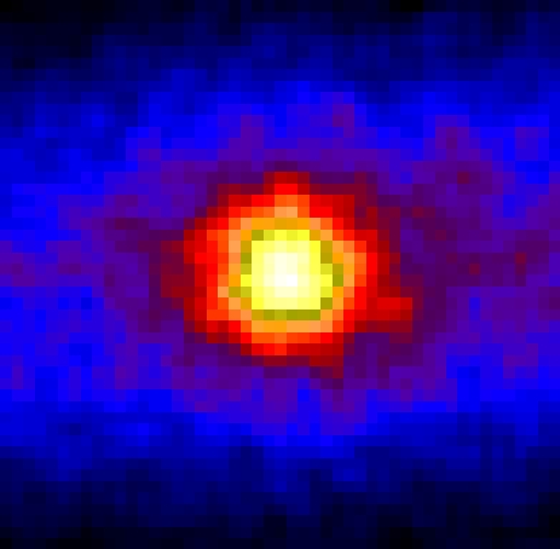
Today, we have also detected neutrinos from our Sun ([3]; see also fig. 1.1), from nuclear decay deep

in the Earth [4], and even from a nearby supernova [5, 6]. Figure 1.2 shows the fluxes and energy

ranges spanned by known and hypothetical neutrino sources.

Another product of the high-energy processes in the universe are cosmic rays: high-energy

protons and atomic nuclei that are accelerated to energies far beyond that of any particle accelerator

on Earth. These cosmic rays bombard the Earth continuously, producing yet more neutrinos that

rain down upon us from high in our atmosphere.

Given a large enough target, we can detect these high-energy atmospheric neutrinos. The

AMANDA-II neutrino detector employs the huge ice sheet at the South Pole as such a target, and

---

2

Figure 1.1: “Picture” of the Sun in neutrinos, as seen by the Super-Kamiokande neutrino

detector. Image credit: R. Svoboda and K. Gordan.

Figure 1.2: Neutrino fluxes as function of energy (multiplied by E

3

to enhance spectral

features) from various sources, including the cosmic neutrino background from the Big

Bang (CνB), supernovae neutrinos (SN ν), solar neutrinos, and atmospheric neutrinos

(from [7]).

---

3

uses sensitive light sensors deep in the ice to detect the light emitted by secondary particles produced

when a neutrino occasionally hits the ice or the bedrock. AMANDA-II accumulates such neutrinos at

the rate of about 16 per day, about four of which are sufficiently high quality to use for an analysis.

Why study these neutrinos? Nature provides a laboratory with energies far above what we

can currently produce on Earth, and studying these high-energy neutrinos can possibly reveal hints

of surprising new physical effects. We know that our theories of gravity and quantum mechanics are

mutually incompatible, but we have no theory of quantum gravity to unify the two. At high enough

energies, we should be able to probe effects of quantum gravity, and neutrinos may prove crucial to

this effort.

In this work, we examine atmospheric neutrinos detected by AMANDA-II from the years 2000

to 2006 for evidence of quantum gravitational effects, by determining their direction and approximate

energy. We have found no evidence for such effects, leading us to set limits on the size of any violations

of our existing theories. Finally, we determine the atmospheric neutrino flux as a function of energy,

extending measurements by other neutrino experiments.

---

4

Chapter 2

Cosmic Rays and Atmospheric Neutrinos

2.1 Cosmic Rays

Cosmic rays are protons and heavier ionized nuclei with energies up to 10

20

eV that constantly

bombard the Earth’s atmosphere. Exactly where they come from and how they are accelerated

to such incredible energies are both open questions. Nearly 100 years after Victor Hess’s balloon

experiments in 1912 showed that cosmic rays come from outer space [8], we still do not know their

source. One of the main difficulties is that the magnetic field of the Galaxy scrambles any directional

information that might point back to a source. Still, all but the highest-energy cosmic rays come

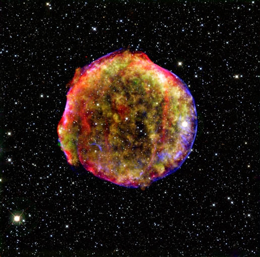
from within our Galaxy, and the expanding shocks around supernovae remnants are a likely candidate

acceleration site [9]. Figure 2.1 shows a composite image of the expanding shock wave around the

Tycho supernova remnant.

The cosmic ray energy spectrum is a power law with differential flux approximately propor-

tional to E

? 2.7

[11]. Figure 2.2 shows measurements of the flux from both direct measurements

(space- and balloon-based instruments) and indirect measurements (air shower arrays). Above about

10

6

GeV, the spectrum steepens to approximately dN/dE ∝ E

? 3

, a feature known as the knee. The

exact mechanism for this transition is unknown, but one possibility is a rigidity-dependent cutoff of

the spectrum as cosmic rays diffuse out of the Galaxy [12].

---

5

Figure 2.1:

X-ray and infrared multi-band image of Tycho’s supernova remnant

(SN 1572), a possible source of galactic cosmic ray acceleration [10]. Image credit:

MPIA/NASA/Calar Alto Observatory.

---

6

10

-10

10

-8

10

-6

10

-4

10

-2

10

0

10

0

10

2

10

4

10

6

10

8

10

10

10

12

E

2

dN/dE

(GeV cm

-2

sr

-1

s

-1

)

E

kin

(GeV / particle)

Energies and rates of the cosmic-ray particles

protons only

all-particle

electrons

positrons

antiprotons

CAPRICE

BESS98

AMS

Ryan et al.

Grigorov

JACEE

Akeno

Tien Shan

MSU

KASCADE

CASA-BLANCA

DICE

HEGRA

CasaMia

Tibet

AGASA

HiRes

Figure 1. Global view of the cosmic-ray spectrum.

would be an increase in the relative abundance of heavy nuclei as first protons, then helium,

then carbon, etc. reach an upper limit on total energy per particle [17]. The first evidence of

such a sequence (which I call a “Peters cycle” [1]) is provided by the recent publication of the

KASCADE experiment [21], which was discussed extensively at this workshop. The data from

KASCADE are limited in energy to below 10

17

eV. The larger KASCADE Grande array [22],

which encloses an area of one square kilometer, will extend the reach of this array to 10

18

eV.

KASCADE measures the shower size at the ground, separately for protons and for GeV muons.

Inferences from the measurements about primary composition depend on simulations of showers

through the atmosphere down to the sea level location of the experiment.

17

Figure 2.2: The cosmic ray energy spectrum as measured by various direct and indirect

experiments, from [13]. The flux has been multiplied by E

2

to enhance features in the

steep power-law spectrum.

---

7

2.2 Atmospheric Neutrinos and Muons

2.2.1 Production

As cosmic rays interact with air molecules in the atmosphere, a chain reaction of particle

production (and decay) creates an extensive air shower of electrons, positrons, pions, kaons, muons,

and neutrinos. Atmospheric neutrinos are produced through hadronic interactions generating charged

pions and kaons, which then decay into muons and muon neutrinos:

π

+

(K

+

) → µ

+

+ ν

µ

(2.1)

π

?

(K

?

) → µ

?

+ ν¯

µ

.

(2.2)

Some of the muons produced in the decay will also eventually decay via exchange of a W

±

boson,

producing both electron and muon neutrinos:

µ

+

→ ν¯

µ

+ e

+

+ ν

e

(2.3)

µ

?

→ ν

µ

+ e

?

+ ν¯

e

.

(2.4)

However, many of these atmospheric muons will survive to ground level and, depending on their

energy, can penetrate kilometers into the Earth before decaying. The process of atmospheric muon

and neutrino production is shown schematically in fig. 2.3.

2.2.2 Energy Spectrum and Angular Distribution

Atmospheric muon neutrinos dominate over all other neutrino sources in the GeV to TeV

energy range. The flux of atmospheric electron neutrinos is over one order of magnitude smaller than

the flux of muon neutrinos at these energies [15]. While the flux of parent cosmic rays is isotropic,

the kinematics of the meson interaction and decay in the atmosphere alters the angular distribution

of atmospheric ν

µ

to a more complicated function of the zenith angle.

While elaborate three-dimensional calculations exist for the expected flux of atmospheric neu-

trinos [16, 17], an approximate analytic formulation is given by Gaisser [11]:

---

8

?

0

?

?

?

?

?

?

?

?

?

?

!

!

?

e

e

?

e

?

e

?

e

?

Decay

Decay

?

?

?

?

?

?

?

?

?

e

Hadronic

shower

Cosmic

ray

Electromagnetic

shower

?

?

! ?

?

? ?

?

?

?

?

!

e

?

? ?

?

e

? ?

?

?

?

! ?

?

? ?

?

?

?

!

e

?

? ?

e

? ?

?

?

rays and

can

). In the

a

?

?

,

?

0

hadronic

0

decays

to the

and

The result of the Kamiokande experiment will be tested in the near future by

super-Kamiokande, which will have significantly better statistical precision. Also,

the neutrino oscillation hypothesis and the MSW solution will be tested by the

Sudbury Neutrino Observatory (SNO) experiment, which will measure both

charged- and neutral-current solar-neutrino interactions.

Figure 2.3: Atmospheric muon and neutrino production (from [14]).

---

9

dN

dE

ν

= C

?

A

πν

1 + B

πν

cos θ

∗

E

ν

/?

π

+ 0.635

A

Kν

1 + B

Kν

cos θ

∗

E

ν

/?

K

?

,

(2.5)

where

A

πν

= Z

Nπ

(1 ? r

π

)

γ

γ +1

(2.6)

and

B

πν

=

γ +2

γ +1

1

1 ? r

π

Λ

π

? Λ

N

Λ

π

ln(Λ

π

/Λ

N

)

.

(2.7)

Equivalent expressions hold for A

Kν

and B

Kν

. In the above, γ is the integral spectral index (so

γ ≈ 1.7); Z

ij

is the spectral-weighted moment of the integral cross section for the production of

particle j from particle i; Λ

i

is the atmospheric attenuation length of particle i; ?

i

is the critical

energy of particle i, at which the decay length is equal to the (vertical) interaction length; r

i

is the

mass ratio m

µ

/m

i

; and cos θ

∗

is not the zenith angle θ at the detector, but rather the angle at the

production height in the atmosphere.

The cosine of the atmospheric angle is roughly equal to that of the zenith angle for cos θ ≥ 0.5.

For steeper angles, we have a polynomial parametrization of the relation that averages over muon

production height [18],

cos θ

∗

=

?

cos

2

θ + p

2

1

+ p

2

(cos θ)

p

3

+ p

4

(cos θ)

p

5

1+ p

2

1

+ p

2

+ p

4

(2.8)

where the fit constants for our specific detector depth are given in table 2.1.

Table 2.1: Fit parameters for the cos θ

∗

correction (eq. 2.8), from [18].

p

1

0.102573

p

2

-0.068287

p

3

0.958633

p

4

0.0407253

p

5

0.817285

While significant uncertainties exist in some of the hadronic physics (especially production of

---

10

log

10

E

ν

/ GeV

1.5

2

2.5

3

3.5

4

-1

sr

-1

s

-2

cm

-1

/dE / GeV

Φ

d

10

log

-14

-13

-12

-11

-10

-9

-8

-7

-6

-5

Barr et al.

Honda et al.

cos

θ

-1

-0.5

0

0.5

1

-1

sr

-1

s

-2

cm

-1

/dE / GeV

Φ

d

10

log

-11

-10.9

-10.8

-10.7

-10.6

-10.5

-10.4

-10.3

-10.2

-10.1

-10

Barr et al.

Honda et al.

Figure 2.4: Predicted atmospheric neutrino flux as a function of energy and zenith angle,

extended to high energies with the Gaisser parametrization. The flux vs. energy (left) is

averaged over all angles, while the flux vs. zenith angle (right) is at 1 TeV.

K

±

and heavier mesons), eq. 2.5 is a useful parametrization of the flux in the energy range where

neutrinos from muon decay can be neglected (E

ν

of at least a few GeV, and higher for horizontal

events).

We can also use eq. 2.5 to extend the detailed calculations of Barr et al. [16] and Honda et al.

[17] to energies of 1 TeV and above, by fitting the parameters in an overlapping energy region (below

700 GeV). We show the extended fluxes for each of these models in fig. 2.4 as a function of energy

and zenith angle.

2.3 Neutrino Oscillations

If neutrinos are massive, their mass eigenstates do not necessarily correspond to their flavor

eigenstates. As we will show, this implies that neutrinos can change flavor as they propagate, and a

ν

µ

produced in the atmosphere may appear as some other flavor by the time it reaches our detector.

In general, there exists a unitary transformation U from the mass basis to the flavor basis.

For oscillation between just two flavors, say ν

µ

and ν

τ

, the transformation can be represented as a

rotation matrix with one free parameter, the mixing angle θ

atm

:

---

11









ν

µ

ν

τ









=









cos θ

atm

sin θ

atm

? sin θ

atm

cos θ

atm

















ν

1

ν

2









.

(2.9)

For free particles propagating in a vacuum, the neutrino mass (energy) eigenstates evolve according

the equation









ν

1

(t)

ν

2

(t)









=









e

? iE

1

t

0

0

e

? iE

2

t

















ν

1

(t = 0)

ν

2

(t = 0)









.

(2.10)

Combining equations 2.9 and 2.10, and using the approximation that the mass of the neutrino is

small compared to its momentum (so that E

i

≈ p +

m

i

2

2p

), we find









ν

µ

(t)

ν

τ

(t)









= U

f

(t)









ν

µ

(t = 0)

ν

τ

(t = 0)









,

(2.11)

where the time-evolution matrix U

f

(t) in the flavor basis is given by

U

f

(t) =









cos

2

θ

atm

e

? i

m

1

2

t

2p

+ sin

2

θ

atm

e

? i

m

2

2

t

2p

cos θ

atm

sin θ

atm

(e

? i

m

1

2

t

2p

? e

? i

m

2

2

t

2p

)

? cos θ

atm

sin θ

atm

(e

? i

m

1

2

t

2p

? e

? i

m

2

2

t

2p

) cos

2

θ

atm

e

? i

m

1

2

t

2p

+ sin

2

θ

atm

e

? i

m

2

2

t

2p









.

(2.12)

By squaring the appropriate matrix element above, this evolution equation can easily be used

to obtain the probability that a muon neutrino will oscillate into a tau neutrino. Conventionally, the

propagation time is replaced by a propagation length L, and the momentum can be approximated

by the neutrino energy E, resulting in the following expression for the survival (non-oscillation)

probability:

P

ν

µ

→ν

µ

= 1 ?

sin

2

2θ

atm

sin

2

?

∆m

2

atm

L

4E

?

,

(2.13)

where ∆m

2

atm

is the squared mass difference and L is in inverse energy units

1

(we continue this

1

L (GeV

? 1

) = L (m)/(c?) = L (m) · 5.07 × 10

15

m

? 1

GeV

? 1

.

---

12

convention unless noted otherwise).

In practice, for atmospheric neutrinos the zenith angle of the neutrino relative to a detector

serves as a proxy for the baseline L. Specifically, the baseline for a given zenith angle θ is given by

L =

?

R

2

Earth

cos

2

θ + h

atm

(2R

Earth

+ h

atm

) ? R

Earth

cos θ

(2.14)

if the neutrino is produced at a height h

atm

in the atmosphere, and where θ = 0 corresponds to a

vertically down-going neutrino. We assume that the Earth is spherical and set the radius R

Earth

=

6370 km, noting that the difference between the polar radius and equatorial radius is only about 0.3%.

We use an average neutrino production height in the atmospheric ?h

atm

? = 20 km [19]. We note that

any correction for detector depth is smaller than the error from either of these approximations.

A description of oscillation between all three flavors can be obtained as above, except that the

transformation matrix U has a 3 × 3 minimum representation and has four free parameters: three

mixing angles θ

12

, θ

13

, and θ

23

, and a phase δ

13

[20]. Fortunately, because of the smallness of the

θ

13

mixing angle and the “solar” mass splitting ∆m

12

, it suffices to consider a two-neutrino system

in the atmospheric case.

Observations of atmospheric neutrinos by Super-Kamiokande [21], Soudan 2 [22], MACRO

[23], and other experiments have provided strong evidence for mass-induced atmospheric neutrino

oscillations. Observations of solar neutrinos by the Sudbury Neutrino Observatory (SNO) have also

shown that the neutrinos truly change flavor, rather than decay or disappear in some other way [24].

A global fit to oscillation data from Super-Kamiokande and K2K [25] results in best-fit atmospheric

parameters of ∆m

2

atm

= 2.2 × 10

? 3

eV

2

and sin

2

2θ

atm

= 1 [26]. Thus from eq. 2.13, for energies

above about 50 GeV, atmospheric neutrino oscillations cease for Earth-diameter baselines. However,

a number of phenomenological models of physics beyond the Standard Model predict flavor-changing

effects at higher energies that can alter the zenith angle and energy spectrum of atmospheric muon

neutrinos. We consider two of these in the next chapter, violation of Lorentz Invariance and quantum

decoherence.

---

13

Chapter 3

Quantum Gravity Phenomenology

Experimental searches for possible low-energy signatures of quantum gravity (QG) can provide a

valuable connection to a Planck-scale theory. Hints from loop quantum gravity [27], noncommutative

geometry [28], and string theory [29] that Lorentz invariance may be violated or spontaneously broken

have encouraged phenomenological developments and experimental searches for such effects [30, 31].

Space-time may also exhibit a “foamy” nature at the smallest length scales, inducing decoherence of

pure quantum states to mixed states during propagation through this chaotic background [32].

As we will discuss, the neutrino sector is a promising place to search for such phenomena.

Water-based or ice-based Ceˇ renkov neutrino detectors such as BAIKAL [33], AMANDA-II [34],

ANTARES [35], and IceCube [36] have the potential to accumulate large samples of high-energy

atmospheric muon neutrinos. Analysis of these data could reveal unexpected signatures that arise

from QG phenomena such as violation of Lorentz invariance or quantum decoherence.

3.1 Violation of Lorentz Invariance

Many models of quantum gravity suggest that Lorentz symmetry may not be exact [31]. Even

if a QG theory is Lorentz symmetric, the symmetry may still be spontaneously broken in our Universe.

Atmospheric neutrinos, with energies above 100 GeV and mass less than 1 eV, have Lorentz gamma

factors exceeding 10

11

and provide a sensitive test of Lorentz symmetry.

Neutrino oscillations in particular are a sensitive testbed for such effects. Oscillations act as a

“quantum interferometer” by magnifying small differences in energy into large flavor changes as the

neutrinos propagate. In conventional oscillations, this energy shift results from the small differences

---

14

in mass between the eigenstates, but specific types of violation of Lorentz invariance (VLI) can also

result in energy shifts that can generate neutrino oscillations with different energy dependencies.

The Standard Model Extension (SME) provides an effective field-theoretic approach to VLI

[37]. The “minimal” SME adds all coordinate-independent renormalizable Lorentz- and CPT-violating

terms to the Standard Model Lagrangian. Even when restricted to first-order effects in the neutrino

sector, the SME results in numerous potentially observable effects [38, 39, 40]. To specify one particu-

lar model which leads to alternative oscillations at high energy, we consider only the Lorentz-violating

Lagrangian term

1

2

i(c

L

)

µνab

L

a

γ

µ

←→

D

ν

L

b

(3.1)

with the VLI parametrized by the dimensionless coefficient c

L

[39]. L

a

and L

b

are left-handed

neutrino doublets with indices running over the generations e, µ, and τ, and D

ν

is the covariant

derivative with A

←→

D

ν

B ≡ AD

ν

B ? (D

ν

A)B.

We restrict ourselves to rotationally invariant scenarios with only nonzero time components

in c

L

, and we consider only a two-flavor system. The eigenstates of the resulting 2 × 2 matrix c

T T

L

correspond to differing maximal attainable velocity (MAV) eigenstates. That is, eigenstates may

have limiting velocities other than the speed of light and may be distinct from either the flavor or

mass eigenstates. Any difference ∆c in the eigenvalues will result in neutrino oscillations. The above

construction is equivalent to a modified dispersion relationship of the form

E

2

= p

2

c

2

a

+ m

2

c

4

a

(3.2)

where c

a

is the MAV for a particular eigenstate, and in general c

a

?= c [41, 42]. Given that the

mass is negligible, the energy difference between two MAV eigenstates is equal to the VLI parameter

∆c/c = (c

a1

? c

a2

)/c, where c is the canonical speed of light.

The effective Hamiltonian H

±

representing the energy shifts from both mass-induced and VLI

oscillations can be written [43]

---

15

H

±

=

∆m

2

4E

U

θ









? 10

01









U

†

θ

+

∆c

c

E

2

U

ξ









? 10

01









U

†

ξ

(3.3)

with two mixing angles θ (the standard atmospheric mixing angle) and ξ (a new VLI mixing angle).

The associated 2 × 2 mixing matrices are given by

U

θ

=









cos θ sin θ

? sin θ cos θ









(3.4)

and

U

ξ

=









cos ξ

sin ξe

±iη

? sin ξe

?iη

cos ξ









(3.5)

with η representing their relative phase. Solving the Louiville equation for time evolution of the state

density matrix ρ

ρ˙ = ? i[H

±

, ρ]

(3.6)

results in the ν

µ

survival probability. This probability P

ν

µ

→ν

µ

is given by

P

ν

µ

→ν

µ

= 1 ?

sin

2

2Θ sin

2

?

∆m

2

L

4E

R

?

,

(3.7)

where the combined effective mixing angle Θ can be written

sin

2

2Θ =

1

R

2

(sin

2

2θ + R

2

sin

2

2ξ + 2R sin 2θ sin 2ξ cos η) ,

(3.8)

the correction to the oscillation wavelength R is given by

R =

?

1 + R

2

+ 2R(cos 2θ cos 2ξ + sin 2θ sin 2ξ cos η) ,

(3.9)

and the ratio R between the VLI oscillation wavelength and mass-induced wavelength is

---

16

E

ν

/ GeV

log

1

1.5

2

2.5

3

3.5

4

4.5

5

)

μ

ν

→

μ

ν

P(

0

0.2

0.4

0.6

0.8

1

Figure 3.1: ν

µ

survival probability as a function of neutrino energy for maximal baselines

(L ≈ 2R

Earth

) given conventional oscillations (solid line), VLI (dotted line, with n = 1,

sin 2ξ = 1, and ∆δ = 10

? 26

), and QD effects (dashed line, with n = 2 and D

∗

=

10

? 30

GeV

? 1

).

R =

∆c

c

E

2

4E

∆m

2

(3.10)

for a muon neutrino of energy E and traveling over baseline L. For simplicity, the phase η is often

set to 0 or π/2. For illustration, if we take both conventional and VLI mixing to be maximal

(ξ = θ = π/4), this reduces to

P

ν

µ

→ν

µ

(maximal) = 1 ? sin

2

?

∆m

2

L

4E

+

∆c

c

LE

2

?

.

(3.11)

Note the different energy dependence of the two effects. The survival probability for maximal baselines

as a function of neutrino energy is shown in fig. 3.1.

Several neutrino experiments have set upper limits on this manifestation of VLI, including

MACRO [44], Super-Kamiokande [45], and a combined analysis of K2K and Super-Kamiokande data

---

17

[43] (∆c/c < 2.0 × 10

? 27

at the 90% CL for maximal mixing). In previous work, AMANDA-II has

set a preliminary upper limit using four years of data of 5.3 × 10

? 27

[46]. Other neutrino telescopes,

such as ANTARES, are also expected to be sensitive to such effects (see e.g. [47]).

Given the specificity of this particular model of VLI, we wish to generalize the oscillation

probability in eq. 3.7. We follow the approach in [47], which is to modify the VLI oscillation length

L ∝ E

? 1

to other integral powers of the neutrino energy E. That is,

∆c

c

LE

2

→ ∆δ

LE

n

2

,

(3.12)

where n ∈ [1, 3], and the generalized VLI term ∆δ is in units of GeV

? n+1

. An L ∝ E

? 2

energy

dependence (n = 2) has been proposed in the context of loop quantum gravity [48] and in the case

of non-renormalizable VLI effects caused by the space-time foam [49]. Both the L ∝ E

? 1

(n = 1)

and the L ∝ E

? 3

(n = 3) cases have been examined in the context of violations of the equivalence

principle (VEP) [50, 51, 52]. We note that in general, Lorentz violation implies violation of the

equivalence principle, so searches for either effect are related [31].

We also note that there is no reason other than simplicity to formulate the VLI oscillations

as two-flavor, as any full description must incorporate all three flavors, and we know nothing of the

size of the various eigenstate splittings and mixing angles. However, a two-flavor system is probably

not a bad approximation, because in the most general case, one splitting will likely appear first as

we increase the energy. Also, since we will search only for a deficit of muon neutrinos, we do not care

to which flavor the ν

µ

are oscillating (so it need not be ν

τ

).

3.2 Quantum Decoherence

Another possible low-energy signature of QG is the evolution of pure states to mixed states via

interaction with the environment of space-time itself, or quantum decoherence. One heuristic picture

of this phenomenon is the production of virtual black hole pairs in a “foamy” spacetime, created

from the vacuum at scales near the Planck length [53]. Interactions with the virtual black holes may

not preserve certain quantum numbers like neutrino flavor, causing decoherence into a superposition

of flavors.

---

18

Quantum decoherence can be treated phenomenologically as a quantum open system which

evolves thermodynamically. The time-evolution of the density matrix ρ is modified with a dissipative

term

/δHρ

:

ρ˙ = ? i[H, ρ] +

/δHρ

.

(3.13)

The dissipative term representing the losses in the open system is modeled via the technique of

Lindblad quantum dynamical semigroups [54]. Here we outline the approach in ref. [55], to which we

refer the reader for more detail. In this case, we have a set of self-adjoint environmental operators

A

j

, and eq. 3.13 becomes

ρ˙ = ? i[H, ρ] +

1

2

?

j

([A

j

, ρA

j

] + [A

j

ρ, A

j

]) .

(3.14)

The hermiticity of the A

j

ensures the monotonic increase of entropy, and in general, pure states will

now evolve to mixed states. The irreversibility of this process implies CPT violation [56].

To obtain specific predictions for the neutrino sector, there are again several approaches for

both two-flavor systems [57, 58] and three-flavor systems [55, 59]. Again, we follow the approach

in [55] for a three-flavor neutrino system including both decoherence and mass-induced oscillations.

The dissipative term in eq. 3.14 is expanded in the Gell-Mann basis F

µ

, µ ∈ [0, 8], such that

1

2

?

j

([A

j

, ρA

j

] + [A

j

ρ, A

j

]) =

?

µ,ν

L

µν

ρ

µ

F

ν

.

(3.15)

At this stage we must choose a form for the decoherence matrix L

µν

, and we select the weak-coupling

limit in which L is diagonal, with L

00

= 0 and L

ii

= ? D

i

. These D

i

represent the characteristic length

scale over which decoherence effects occur. Solving this system for atmospheric neutrinos (where we

neglect mass-induced oscillations other than ν

µ

→ ν

τ

) results in the ν

µ

survival probability [55]:

---

19

P

ν

µ

→ν

µ

=

1

3

+

1

2

?

1

4

e

? LD

3

(1 + cos 2θ)

2

+

1

12

e

? LD

8

(1 ? 3 cos 2θ)

2

+ e

?

L

2

(D

6

+D

7

)

· sin

2

2θ

cos





L

2

?

?

∆m

2

E

?

2

? (D

6

? D

7

)

2





+

sin

?

L

2

?

?

∆m

2

E

?

2

? (D

6

? D

7

)

2

?

(D

6

? D

7

)

?

?

∆m

2

E

?

2

? (D

6

? D

7

)

2

??

.

(3.16)

Note the limiting probability of

1

3

, representing full decoherence into an equal superposition of flavors.

The D

i

not appearing in eq. 3.16 affect decoherence between other flavors, but not the ν

µ

survival

probability.

We note that in eq. 3.16, we must impose the condition ∆m

2

/E > |D

6

? D

7

|, but this is not

an issue in the parameter space we explore in this analysis. If one wishes to ensure strong conditions

such as complete positivity [57], there may be other inequalities that must be imposed (see e.g. the

discussion in ref. [59]).

The energy dependence of the decoherence terms D

i

depends on the underlying microscopic

model. As with the VLI effects, we choose a generalized phenomenological approach where we suppose

the D

i

vary as some integral power of the energy,

D

i

= D

∗

i

E

n

, n ∈ [1, 3] ,

(3.17)

where E is the neutrino energy in GeV, and the units of the D

∗

i

are GeV

? n+1

. The particularly

interesting E

2

form is suggested by decoherence calculations in non-critical string theories involving

recoiling D-brane geometries [60]. We show the n = 2 survival probability as a function of neutrino

energy for maximal baselines in fig. 3.1.

An analysis of Super-Kamiokande in a two-flavor framework has resulted in an upper limit

at the 90% CL of D

∗

< 9.0 × 10

? 28

GeV

? 1

for an E

2

model and all D

∗

i

equal [61]. ANTARES

has reported sensitivity to various two-flavor decoherence scenarios as well, using a more general

formulation [58]. Analyses of Super-Kamiokande, KamLAND, and K2K data [62, 63] have also set

---

20

strong limits on decoherence effects proportional to E

0

and E

? 1

. Because our higher energy range

does not benefit us for such effects, we do not expect to be able to improve upon these limits, and

we focus on effects with n ≥ 1.

Unlike the VLI system, we have used a full three-flavor approach to the phenomenology of the

QD system. There is no theoretical justification for doing so in one but not the other, but for the

special case in which all decoherence parameters are equal, the choice is important. This is because

in a three-flavor system, the limiting survival probability is 1/3, compared to 1/2 in a two-flavor

system. Since heuristically the equality of decoherence parameters suggests that the interactions

with space-time are flavor-agnostic, we feel that using a three-flavor description is more apt.

---

21

Chapter 4

Neutrino Detection

4.1 General Techniques

A major obstacle to overcome in the detection of the neutrino is its small cross section: while

the neutrino-nucleon cross section rises with energy, at 1 TeV the interaction length is still 2.5 million

kilometers of water [64]. Thus, any potential detector must encompass an enormous volume to achieve

a reasonable event rate. Once an interaction does occur in or near the detector, we can detect the

resulting charged particles by means of their radiation. A (relatively) cost-effective approach is to

use natural bodies of water or transparent ice sheets as the target material, and then instrument this

volume with photomultiplier tubes. While originally proposed in 1960 by K. Greisen and F. Reines

[65, 66], large-scale detectors of this sort have only been in operation for the past decade or so.

Water or ice neutrino detectors typically consist of vertical cables (called “strings” or “lines”)

lowered either into deep water or into holes drilled in the ice. Photomultiplier tubes (PMTs) in

pressure housings are attached to the cables, which supply power and communications. A charged-

current neutrino interaction with the surrounding matter produces a charged lepton via the process

ν

l

(ν

l

)+ q → l

?

(l

+

)+ q

?

,

(4.1)

where q is a valence or sea quark in the medium, and q

?

is as appropriate for charge conservation.

In the case of a muon neutrino, the resulting muon can travel a considerable distance within the

medium.

---

22

μ

±

ct/n

!ct

"

c

Figure 4.1: Formation of a Ceˇ renkov cone by a relativistic muon moving through a

medium.

4.2 Cˇerenkov Radiation

Because the relativistic muon produced in the neutrino interaction is traveling faster than the

speed of light in the medium, it will radiate via the Ceˇ renkov effect. A coherent “shock wave” of light

forms at a characteristic angle θ

c

depending on the index of refraction n of the medium, specifically,

cos θ

c

=

1

nβ

,

(4.2)

where β = v/c is the velocity of the particle. For ice, where n ≈ 1.33, the Ceˇ renkov angle is about

41

◦

for relativistic particles (β ≈ 1). A full treatment differentiates between the phase and group

indices of refraction, but this is a small correction (see e.g. [67]). Figure 4.1 presents a geometric

derivation of the simpler form shown in eq. 4.2.

The number of Ceˇ renkov photons emitted per unit track length as a function of wavelength λ

is given by the Franck-Tamm formula [68]

d

2

N

dxdλ

=

2πα

λ

2

?

1 ?

1

β

2

n

2

?

,

(4.3)

where α is the fine-structure constant. Because of the 1/λ

2

dependence, the high-frequency photons

dominate the emission, up to the ultraviolet cutoff imposed by the glass of the PMT pressure vessel

---

23

(about 365 nm [69]). Between this and the frequency at which is the ice is no longer transparent

(about 500 nm; see section 5.2), we expect an emission of about 200 photons per centimeter [70].

4.3 Muon Energy Loss

Ceˇ renkov radiation from the bare muon is not its dominant mode of energy loss. The rate of

energy loss as a function of distance, dE/dx, can be parametrized as

?

dE

dx

= a(E) + b(E) E ,

(4.4)

where a(E) is the ionization energy loss given by the standard Bethe-Bloch formula (see e.g. [71]), and

b(E) is the sum of losses by e

+

e

?

pair production, bremsstrahlung, and photonuclear interactions.

The energy losses from various contributions are shown in figure 4.2.

The ionization energy losses are continuous in nature, occurring smoothly along the muon

track. However, at high energies, the losses by bremsstrahlung, pair production, and photonuclear

interactions are not continuous but stochastic: rare events that result in large depositions of energy

via particle and photon creation. The particles produced are highly relativistic, and if charged, they

too will radiate via the Ceˇ renkov effect. Furthermore, because they are kinematically constrained to

the approximate direction of the muon, this emission will peak at the Ceˇ renkov angle of the muon.

The roughly conical Ceˇ renkov emission of the bare muon is thus enhanced by the various energy

losses described above [73].

4.4 Other Event Topologies

For charged-current ν

e

and ν

τ

interactions, or neutral-current interactions of any flavor, the

event topology is less track-like than the muon case described above, and is instead more spherical

or “cascade-like.” For ν

e

events, this is because of the short path length of the resulting electron or

positron within the ice. For ν

τ

events (except for those of very high energy), the resulting τ lepton

will decay immediately, in most cases resulting in a hadronic shower. However, 17% of the time [20],

the τ will decay via

---

24

the question arises whether this precision is sufficient to p

dreds of interactions along their way. Figure 6 is one of

strate that it is sufficient: the final energy distribution did

parametrizations. Moreover, different orders of the inter

responding to the number of the grid points over which

tested (Figure 9) and results of propagation with differ

other (Figure 10). The default value of

g

was chosen to b

other acceptable values 3 ≤

g

≤ 6 at the run time.

ioniz

brems

photo

epair

decay

energy [GeV]

energy losses

[

GeV/(g/cm

2

)

]

10

10

-10

10

-9

10

-8

10

-7

10

-6

10

-5

10

-4

10

-3

10

-2

1

-1

10

10

2

10

3

10

4

10

5

10

6

10

-1

1 10 10

2

10

3

10

4

10

5

10

6

10

7

10

8

10

9

10

10

10

11

precision of parametrization (total)

10

-10

10

-9

10

-8

10

-7

10

-6

10

-5

10

-4

10

-3

10

-2

10

-1

1

10

-1

1 10

Fig. 7. Ionization (upper solid curve),

bremsstrahlung (dashed), photonuclear

(dotted), epair production (dashed-dot-

ted) and decay (lower solid curve) losses

in ice

Fig.

8.

(e

pa

− e

np

)/

g=2

g=3

g=4

g=5

-3

10

-2

10

-1

1

g=5

g=3

10

4

10

5

0 10 20

Figure 4.2: Average muon energy loss in ice as a function of energy, from [72].

---

25

τ

+

→ µ

+

+ ν

µ

+ ν¯

τ

τ

?

→ µ

?

+ ν¯

µ

+ ν

τ

,

(4.5)

possibly resulting in a detectable muon track (albeit of significantly lower energy than the original

ν

τ

). For a neutral-current event, there is no outgoing charged lepton, although there may be a

hadronic shower from the collision.

Because cascade-like and track-like events have very different signatures and strategies for

background rejection, one generally focuses on one or the other early in the analysis. We consider

only ν

µ

-induced muons in this analysis; other types of event will be removed by the data-filtering

procedures which we describe in chapter 6.

4.5 Background

While we have described the means by which we might detect a neutrino-induced muon,

the background to such a search is formidable. Even with kilometers of overburden, high-energy

atmospheric muon bundles dominate over neutrino events by a factor of about 10

6

. Selecting only

“up-going” muons allows us to reject the large background of atmospheric muons, using the Earth

as a filter to screen out everything but neutrinos (see fig. A.2). In practice, we must also use other

observables indicating the quality of the muon directional reconstruction, in order to eliminate mis-

reconstructed atmospheric muon events — a topic we will revisit in chapter 6.

---

26

Chapter 5

The AMANDA-II Detector

5.1 Overview

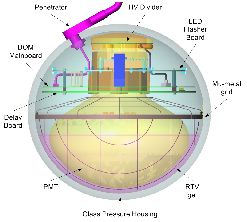
AMANDA, or the Antarctic Muon And Neutrino Detector Array, consists of 677 optical

modules (OMs) on 19 vertical cables or “strings” frozen into the deep, clear ice near the geographic

South Pole. Each OM consists of an 8” diameter Hamamatsu R5912-2 photomultiplier tube (PMT)

housed in a glass pressure sphere. The AMANDA-II phase of the detector commenced in the year

2000, after nine outer strings were added. Fig. 5.1 shows the geometry of the detector, as well as the

principal components of the OMs.

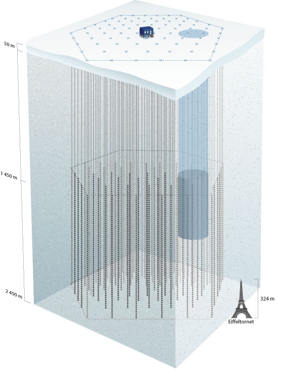
The bulk of the detector lies between 1550 and 2050 meters under the snow surface, where the

Antarctic ice sheet is extremely clear. The 19 strings are arranged roughly in three concentric cylin-

ders, the largest of which is approximately 200 meters in diameter. The OMs are connected to cables

which supply power and transmit PMT signals to the surface. Multiple cabling technologies are used:

coaxial, twisted-pair, and fiber optic. While most transmitted signals are analog, string 18 contains

prototype digital optical modules (DOMs) which digitize the PMT signal before transmission.

5.2 Optical Properties of the Ice

Far from being a homogeneous medium, the ice at the South Pole consists of roughly horizontal

layers of varying clarity. As the ice layers accumulated over geological time periods, varying amounts

of atmospheric dust were trapped during the deposition, depending on the climatological conditions

at the time. These “dust layers” strongly affect both the optical scattering and absorption lengths

---

27

Section 6 summarizes event classes for which the

reconstruction may fail and strategies to identify

and eliminate such events. The performance

of the reconstruction procedure is shown in

Section 7. We discuss possible improvements

in Section 8.

2. The AMANDA detector

The AMANDA-II detector (see Fig. 2) has been

operating since January 2000 with 677 optical

modules (OM) attached to 19 strings. Most of the

OMs are located between 1500 and 2000 m below

and Refs. [8,9]), while providing SPASE with

additional information for cosmic ray composition

studies [10].

The PMT signals are processed in a counting

room at the surface of the ice. The analog signals

are amplified and sent to a majority logic trigger

[11]. There the pulses are discriminated and a

trigger is formed if a minimum number of hit

PMTs are observed within a time window of

typically 2 ms: Typical trigger thresholds were 16

hit PMT for AMANDA-B10 and 24 for AMANDA-II.

For each trigger the detector records the peak

amplitude and up to 16 leading and trailing edge

times for each discriminated signal. The time

ARTICLE IN PRESS

light diffuser ball

HV divider

Module

Optical

pressure

housing

Depth

AMANDA-II

AMANDA-B10

Inner 10 strings:

zoomed in on one

optical module (OM)

main cable

PMT

200 m

1000 m

2350 m

2000 m

1500 m

1150 m

Fig. 2. The AMANDA-II detector. The scale is illustrated by the Eiffel tower at the left.

172

J. Ahrens et al. / Nuclear Instruments and Methods in Physics Research A 524 (2004) 169–194

Section 6 summarizes event classes for which the

reconstruction may fail and strategies to identify

and eliminate such events. The performance

of the reconstruction procedure is shown in

Section 7. We discuss possible improvements

in Section 8.

2. The AMANDA detector

The AMANDA-II detector (see Fig. 2) has been

operating since January 2000 with 677 optical

and Refs. [8,9]

), while providing SPASE with

additional information for cosmic ray composition

studies [10].

The PMT signals are processed in a counting

room at the surface of the ice. The analog signals

are amplified and sent to a majority logic trigger

[11]. There the pulses are discriminated and a

trigger is formed if a minimum number of hit

PMTs are observed within a time window of

typically 2 ms: Typical trigger thresholds were 16

hit PMT for AMANDA-B10 and 24 for AMANDA-II

For each trigger the detector records the peak

amplitude and up to 16 leading and trailing edge

ARTICLE IN PRESS

light diffuser ball

HV divider

Module

Optical

pressure

housing

Depth

AMANDA-II

AMANDA-B10

Inner 10 strings:

zoomed in on one

optical module (OM)

main cable

PMT

200 m

1000 m

2350 m

2000 m

1500 m

1150 m

Fig. 2. The AMANDA-II detector. The scale is illustrated by the Eiffel tower at the left.

172

J. Ahrens et al. / Nuclear Instruments and Methods in Physics Research A 524 (2004) 169–194

Section 6 summarizes event classes for which the

reconstruction may fail and strategies to identify

and eliminate such events. The performance

of the reconstruction procedure is shown in

Section 7. We discuss possible improvements

in Section 8.

2. The AMANDA detector

The AMANDA-II detector (see Fig. 2) has been

operating since January 2000 with 677 optical

modules (OM) attached to 19 strings. Most of the

OMs are located between 1500 and 2000 m below

and Refs. [8,9]

), while providing SPASE with

additional information for cosmic ray composition

studies [10].

The PMT signals are processed in a counting

room at the surface of the ice. The analog signals

are amplified and sent to a majority logic trigger

[11]. There the pulses are discriminated and a

trigger is formed if a minimum number of hit

PMTs are observed within a time window of

typically 2 ms: Typical trigger thresholds were 16

hit PMT for AMANDA-B10 and 24 for AMANDA-II

For each trigger the detector records the peak

amplitude and up to 16 leading and trailing edge

times for each discriminated signal. The time

ARTICLE IN PRESS

light diffuser ball

HV divider

Module

Optical

pressure

housing

Depth

AMANDA-II

AMANDA-B10

Inner 10 strings:

zoomed in on one

optical module (OM)

main cable

PMT

200 m

1000 m

2350 m

2000 m

1500 m

1150 m

Fig. 2. The AMANDA-II detector. The scale is illustrated by the Eiffel tower at the left.

172

J. Ahrens et al. / Nuclear Instruments and Methods in Physics Research A 524 (2004) 169–194

Figure 5.1: Diagram of the AMANDA-II detector with details of an optical module (from

[74]). The Eiffel tower on the left illustrates the scale.

---

28

and must be taken into account for event reconstruction and simulation.

The scattering and absorption properties have been measured or inferred using a number of

in situ light sources [75], resulting in a comprehensive model of the ice properties known as the

“Millennium” ice model. Since the publication of that work, the effect of smearing between dust

layers has been examined, resulting in an updated model of the ice known as “AHA.” The effective

scattering length in this model λ

eff

s

, defined such that

λ

eff

s

=

λ

s

1 ? ? cos θ

s

?

,

(5.1)

with an average scattering angle of ?cos θ

s

? ≈ 0.95, is shown along with the absorption length λ

a

in

fig. 5.2. The effective scattering length is approximately 20 m, whereas the absorption length (at 400

nm) is about 110 m.

5.3 Data Acquisition and Triggering

Cables from the deep ice are routed to surface electronics housed in the Martin A. Pomerantz

Observatory (MAPO). PMT signals, broadened after transmission to the surface, are amplified in

Swedish amplifiers (SWAMPs). A prompt output from the SWAMPs is fed to a discriminator,

which in turn feeds the trigger logic and a time-to-digital converter (TDC). The TDC records the

leading and falling edges when the signal crosses the discriminator level. Each edge pair forms a hit,

of which the TDC can store eight at a time. The difference between the edges is referred to as the

time-over-threshold, or TOT.

The main trigger requires 24 hit OMs within a sliding window of 2.5 µs. The hardware core

of the trigger logic is formed by the digital multiplicity adder-discriminator (DMADD). When the

trigger is satisfied, the trigger electronics open the gate to a peak-sensing analog-to-digital converter

(ADC) which is fed by a delayed signal from the SWAMPs. The ADC gate remains open for 9.8 µs,

and the peak amplitude during that window is assigned to all hits in that particular channel. 10

µs after the trigger, a stop signal is fed to the TDC. The trigger is also sent to a GPS clock which

timestamps the event. Events are recorded to magnetic tape and then flown north during the austral

summer season.

---

29

!"#$%&'()&

!"#$%&'()&

*+,

-

"..&&

'(

/*

)&

*+,

0

&

'(

/*

)&

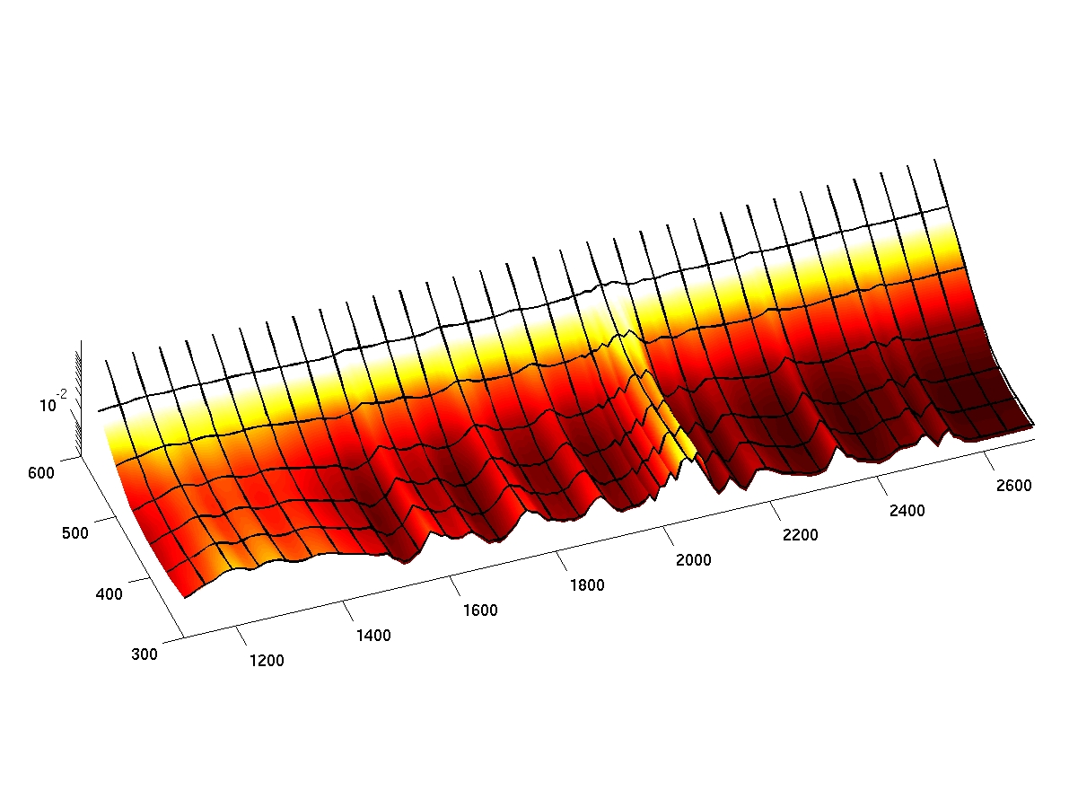
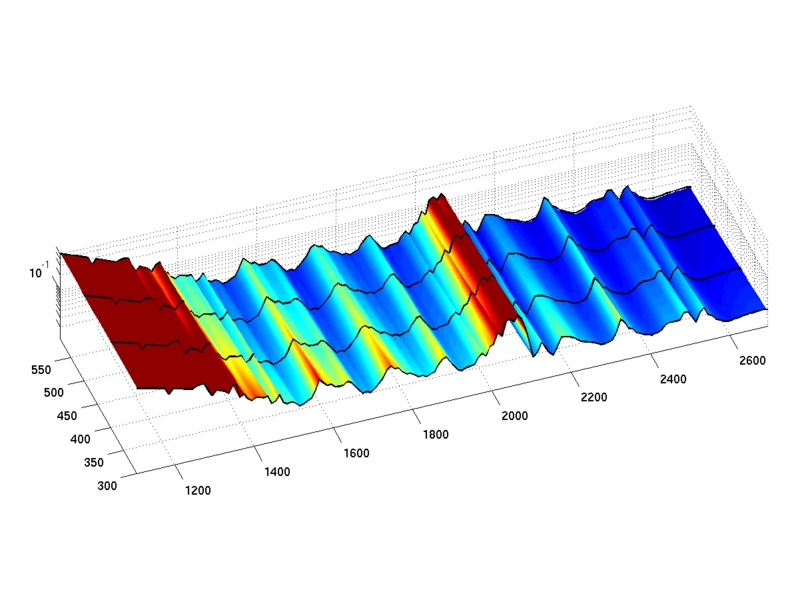
Figure 5.2: Inverse absorption and effective scattering lengths as a function of depth and

wavelength in the AHA ice model. Note the large dust peak at a depth of roughly 2050

m, with three smaller dust peaks at shallower depths.

---

30

SWAMP

~2 km

discriminator

trigger

…

TDC

DMADD

2 μs delay

ADC

gate

stop

c

o

m

p

u

t

e

readout

r

10 μs delay

Figure 5.3: Principal components of the AMANDA µ-DAQ (adapted from [67]).

The data acquisition system (DAQ) described here is known as the muon DAQ, or µ-DAQ, and

operated through 2006. A parallel DAQ that also records waveform information, the TWR-DAQ,

has been fully operational since 2004. Only µ-DAQ data are used in this analysis. A simplified block

diagram showing the principal components in shown in fig. 5.3.

5.4 Calibration

Calibration of cable time delays and the corrections for dispersion are performed with in situ

laser sources. After calibration, the time resolution for the first 10 strings is σ

t

≈ 5 ns (those with

coaxial or twisted-pair cables), and the time resolution for the optical fiber strings is σ

t

≈ 3.5 ns [74].

The time delay calibration is cross-checked using down-going muon data.

The amplitude calibration uses single photoelectrons (SPEs) from low-energy down-going

muons as a “calibration source” of known charge. The uncalibrated amplitude distribution of SPEs

is fit as the sum of an exponential and a Gaussian distribution, with the peak of the Gaussian portion

representing one PE.

---

31

Chapter 6

Simulation and Data Selection

6.1 Simulation

In order to meaningfully compare our data with expectations from various signal hypothe-

ses, we must have a detailed Monte Carlo (MC) simulation of the atmospheric neutrinos and the

subsequent detector response. For the input atmospheric muon neutrino spectrum, we generate an

isotropic power-law flux with the nusim neutrino simulator [76] and then reweight the events to

standard flux predictions [16, 17]. As discussed in section 2.2.2, we have extended the predicted

fluxes to the TeV energy range via the neutrinoflux package, which fits the low-energy region

with the Gaisser parametrization [11] and then extrapolates above 700 GeV. We add standard oscil-

lations and/or non-standard flavor changes by weighting the events with the muon neutrino survival

probabilities in eqs. 2.13, 3.7, or 3.16.

Muon propagation and energy loss near and within the detector are simulated using mmc

[72]. Photon propagation through the ice, including scattering and absorption, is modeled with

photonics [77], incorporating the depth-dependent characteristic dust layers from the AHA ice

model (see section 5.2). The detector simulation amasim [78] records the photon hits, and then

identical filtering and reconstruction methods are performed on data and simulation. Cosmic ray

background rejection is ensured at all but the highest quality levels by a parallel simulation chain fed

with atmospheric muons from corsika [79], although when reaching contamination levels of O(1%)

— a rejection factor of 10

8

— computational limitations become prohibitive.

As we will discuss further in chapter 8, the absolute sensitivity of the OMs is one of the

---

32

larger systematic uncertainties. Determining the effect on our observables can only be achieved by

rescaling the sensitivity within amasim and re-running the detector simulation. We have generated

atmospheric neutrino simulation for 7 different optical module sensitivities, and for each set we reach

an effective livetime (see appendix D) of approximately 60 years.

6.2 Filtering and Track Reconstruction

Filtering the large amount of raw AMANDA-II data from trigger level to neutrino level is an

iterative procedure. First, known bad optical modules are removed, resulting in approximately 540

OMs for use in the analysis. Unstable or incomplete runs (“bad files”) are identified and excluded.

Hits caused by electrical crosstalk and isolated noise hits are also removed (“hit cleaning”).

The initial data volume is so large that only fast, first-guess algorithms can be run on all events.

These include the direct walk algorithm [74] and JAMS [80], both of which employ pattern-matching

algorithms to reconstruct muon track directions. If the zenith angle is close to up-going (typically

greater than 70

◦

or 80

◦

), the event is kept in the sample. This step is known as “level 1” or L1

filtering. “Level 2” and “level 3” filtering steps consist of more computationally intensive directional

reconstructions, along with another zenith angle cut using the more accurate results.

The best angular resolution is achieved by likelihood-based reconstructions utilizing the timing

information of the photon hits. The iterative unbiased likelihood (UL) reconstruction uses the timing

of the first hit in an OM, and maximizes the likelihood

L =

?

i

p(t

i

|?a) ,

(6.1)

where ?a = (x, y, z, θ, φ) is the track hypothesis and t

i

is the timing residual for hit i. The timing

residual is the difference between the expected photon arrival time based only on geometry and the

actual arrival time, which in general is delayed by scattering in the ice. A parametrization of the

probability distribution function describing the time residuals of the first photon hits is given by the

Pandel function

1

[81], and this is convoluted with a Gaussian to include PMT jitter. A high-quality

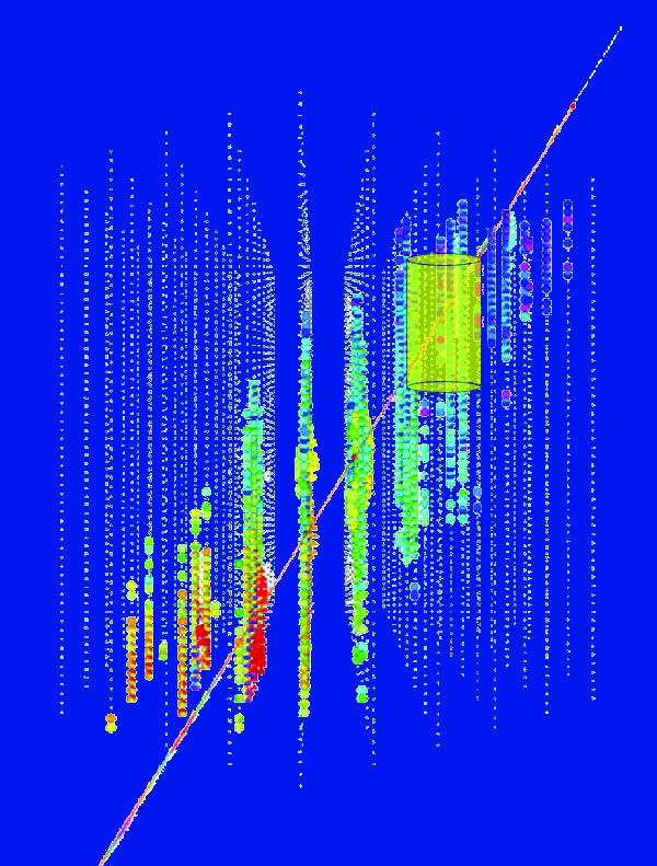
sample event is shown in fig. 6.1 along with the track from the UL reconstruction.

1

For this reason, the UL reconstruction is also commonly referred to as the “Pandel” reconstruction (even though

other reconstructions also use the Pandel p.d.f.). We use the terms interchangeably.

---

33

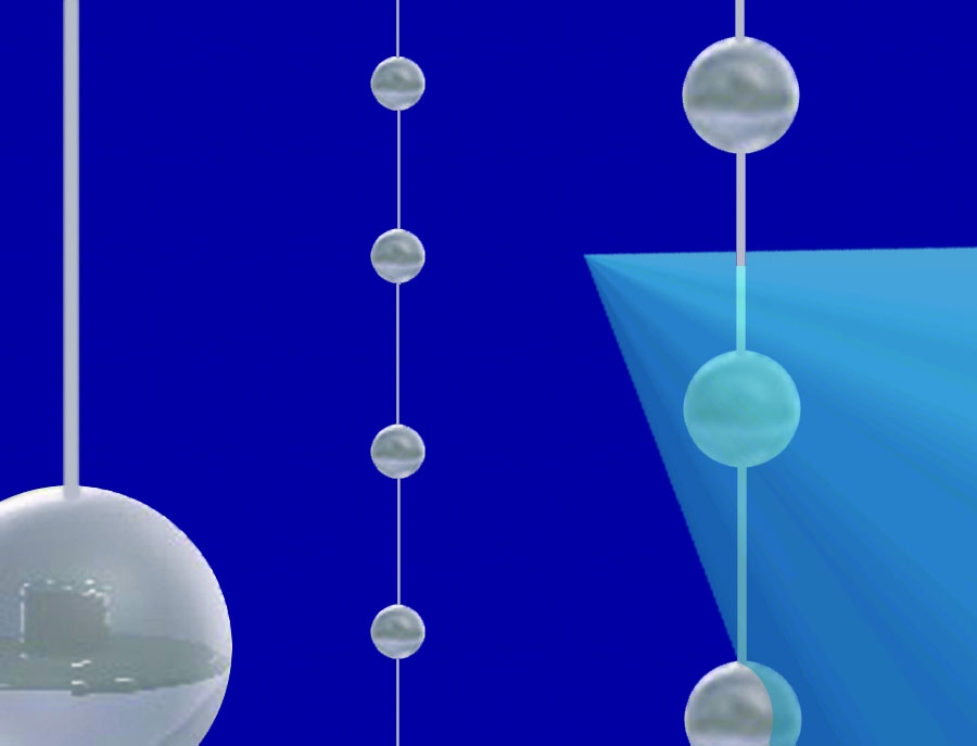
Figure 6.1: Sample AMANDA-II event from 2001, with number of OMs hit N

ch

= 77.

Colors indicate the timing of the hits, with red being earliest. The size of the circles

indicate the amplitude of the PMT signal. The line is the reconstructed track obtained

from the unbiased likelihood or “Pandel” fit (σ = 1.2

◦

).

---

34

Because we are interested in rejecting atmospheric muons, it is useful to compare the UL

likelihood with a reconstruction using the prior hypothesis that the event is down-going. This

Bayesian likelihood (BL) reconstruction weights the likelihood with the prior probability density

function (PDF) P

µ

(θ), a polynomial fit to the zenith-angle dependence of the muon flux at the depth

of the AMANDA-II detector. The likelihood to maximize therefore becomes

L

Bayes

=

?

i

p(t

i

|?a) P

µ

(θ) .

(6.2)

The log-likelihood ratio of the UL fit to the BL fit is then a test statistic which we can use as a

quality parameter.

6.3 Quality Cuts

After initial filtering and reconstruction (after level 3), atmospheric neutrino events are still

dominated by mis-reconstructed atmospheric muons (down-going muons that are incorrectly recon-

structed as up-going). In order to remove (or “cut”) these events, we must use several variables

indicating the quality of the track reconstruction.

6.3.1 Point-source Cuts

As a starting point for these quality cuts, we use the criteria developed for the 2000-2004

AMANDA-II point source analysis [82]. These cuts are applicable to an atmospheric neutrino analysis

primarily because they are not optimized for a high-energy extraterrestrial neutrino flux, and so their

efficiency for lower-energy atmospheric neutrinos is still quite good. These cuts are shown in table

6.1.

6.3.1.1 Likelihood Ratio

As described in section 6.2, the log likelihood ratio log L

UL

/L

BL

tests the relative probability

of the unbiased “Pandel” fit (which, because of the zenith-angle cuts, indicates the track is up-going

or close to it), and the Bayesian down-going fit. The larger this ratio, the less likely the event is to

be down-going. Including a dependence on the zenith angle is necessary because this test gets less

powerful near the horizon, where the up-going and down-going tracks may only be separated by a

---

35

Table 6.1: Initial quality cuts, originally designed for the 2000-2004 point-source analysis.

x = sin δ

UL

, where δ is the reconstructed declination, and Θ() is the unit step function.

Quality variables are described in the text.

Description

Criterion (to keep)

Likelihood ratio log L

UL

/L

BL

> 34 + 25(1 ? Θ(x ? 0.15)) · (x ? 0.15)

Smoothness

|S

Phit,UL

| < 0.36 and S

Phit,UL

?= 0

Paraboloid error

σ < 3.2

◦

? 4

◦

· Θ(x ? 0.75) · (x ? 0.75) and σ ?= 0

Flariness

F

TOT-short

+ F

B10

+ F

B10

< 10

Stability period

2000: day ∈ [47, 309]

2001: day ∈ [44, 293]

2002: day ∈ [43, 323]

2003: day ∈ [43, 315]

2004: day ∈ [43, 309]

2005-06: included in file selection

File size

2000-04: Runs/file > 6

Bayesian bug fix

2005-06: θ

BL

< 90

◦

small angle.

6.3.1.2 Smoothness

The smoothness of a track hypothesis is a topological parameter varying from -1 to 1 that

measures the evenness of the hits along the track. Positive values of the smoothness indicate hits

concentrated at the beginning of the track, while negative values indicate hits concentrated at the

end. Small absolute value of the smoothness indicates that the hits are more evenly distributed,

supporting the fit hypothesis.

The particular implementation of the smoothness calculation that we use, the P

hit

smoothness

or S

Phit

, only considers direct (unscattered) hits within a 50 m cylinder around the UL track. It

then compares the number of hits in the cylinder to the number expected given a minimally ionizing

muon (see ref. [80] for more detail). In table 6.1, we also explicitly exclude events with exactly zero

smoothness; in an early implementation, this result indicated no direct hits within the cylinder.

6.3.1.3 Paraboloid Error

The paraboloid error, or angular resolution parameter, is an estimate of the 1σ error on the

direction of the UL fit, and poorly reconstructed tracks will tend to have higher values of this error.

This parameter is obtained by fitting a paraboloid to the likelihood space near the best-fit minimum

---

36

[83]. Using the fit to approximate the 1σ confidence level results in an error ellipse with major and

minor axes σ

1

and σ

2

, and we form with these a single error parameter σ by taking the geometric

mean

σ =

√

σ

1

σ

2

.

(6.3)

The quality cut on the paraboloid error is tightened near the horizon, where background

contamination worsens. Pathological results, such as zero or negative values of the ellipse axes, must

be excluded.

6.3.1.4 Flariness and Stability Period

In periods of windy or stormy weather at the South Pole, electrical induction on the surface

cables (especially twisted-pair cables) can actually result in enough spurious “hits” to trigger the

detector. These types of fake events are known as flares, and to enable removal of these events, a

number of characteristic flare variables have been developed [84]. We use three of these flare variables:

F

TOT-short

, the number of hits in twisted-pair channels with TOT shorter than expected; F

B10

, the

ratio of hits in strings 1-4 (coaxial cabling) to strings 5-10 (twisted-pair cabling); and F

B10

, the ratio

of hits in strings 11-19 with optical cabling to those with twisted-pair cabling. The flare indicators

are normalized as logarithms of probabilities, so we use their sum as a combined flare indicator.

Finally, since configuration changes often take place during the austral summer season, we

exclude these periods with a stability period cut based on the day of the year of the event. This is

only necessary for data from 2000-2004, as for 2005 and 2006 this was performed as part of the file

selection before the initial data filtering.

6.3.2 Purity Cuts

After applying the cuts described in the previous section, we can examine the purity of the

sample using a cut-tightening ratio procedure, and then try to isolate any remaining background

events. First, we uniformly tighten or loosen all the cut parameters by scaling them linearly with a

“cut strength” parameter. We multiply the observable x by either α or 1/α depending on the cut:

---

37

Cut strength

0.9

0.95

1

1.05

1.1

1.15

1.2

Data/MC ratio

1.05

1.1

1.15

1.2

1.25

1.3

1.35

1.4

1.45

Data/MC ratio vs. cut strength (2000-2006, 1=Zeuthen cuts)

Figure 6.2: Data/MC ratio as a function of cut strength (1 = point-source cuts). The

dashed line indicates the average of the flat region.

(x

i

<X

0

) → (αx

i

<X

0

) ,

(6.4)

(x

i

> X

0

) →

?

x

i

α

> X

0

?

∀ i .

Figure 6.2 shows the result of this procedure. As the cuts are tightened, the background is eventually

eliminated, leaving only a systematic normalization shift in the simulation. After performing this

procedure using the point-source cuts, we find that there is a background contamination of 2-3% (the

difference between the ratio at the nominal cuts, cut strength=1, and the ratio in the flat region).

As we will see, however, this procedure is not foolproof; it only eliminates background at the tails of

the quality parameters we are already using.

We have isolated several parameters which are of use to reduce this background even further:

• Ψ, the space angle between the Pandel/UL and JAMS fits;

• N

dirC

, the number of direct hits (class C, with t

res

∈ [? 15, 75] ns); and

• L

dirB

, the maximum separation along the track of direct hits (class B, with timing residual

t

res

∈ [? 15, 25] ns).

---

38

In each of these variables, there are tails in the data that are not matched by atmospheric neutrino

simulation but are consistent with mis-reconstructed muons. This is shown in fig. 6.3, along with the

region we have chosen to eliminate. These purity cuts are also shown in table 6.2.

Table 6.2: Purity cuts designed to remove the remaining background contamination after

applying the quality cuts shown in table 6.1.

Description Criterion (to keep)

Up-going

cos θ

UL

< 0

Space angle

Ψ

UL,JAMS

< 25

◦

Direct hits

N

dirC

> 6

Direct length

L

dirB

> 60 m

After reapplying the same cut-tightening ratio procedure described above, we estimate that

these cuts achieve a purity of greater than 99%. This reduces the data from 6099 to 5686 events

(-7%) while reducing the atmospheric neutrino MC prediction by 2%. However, this turns out to be

an overestimation of the purity.

6.3.3 High-N

ch

Excess and Additional Purity Cuts

The selection criteria described above, as well as the analysis procedure described in chapter

7, were designed blindly. Specifically, our observables (the zenith angle and number of OMs hit, N

ch

;

see section 7.1) were hidden until the cuts and analysis procedures were finalized. However, after

unblinding, we examined the N

ch

and cos θ

UL

distributions and found an unexpected 1.5% excess in

the (60 < N

ch

< 120) region (see fig. 6.4). This is slightly higher than the estimated 0.5% background

contamination, and more importantly, it is not distributed evenly across the observable space (which

is how we model background contamination in the systematic errors). In this section, we discuss the

impact of the excess, and how we have chosen to address it.

An analysis of the events in the high-N

ch

region suggests that the excess (about 85 events

compared to Monte Carlo normalized to the low-N

ch

region) consists of mis-reconstructed muons.

Salient observations about the excess include:

• the excess is evenly spread across all years;

• events scanned in the event viewer are not track-like (perhaps muon bundles passing outside

---

39

hMC0

Entries 274785

Integral

5529

!

Pandel-JAMS

(degrees)

0

20

40

60

80

100 120 140 160

180

10

-2

10

-1

1

10

10

2

10

3

hMC0

Entries 274785

Integral

hData

Entries 6099

Integral

hData

Entries 6099

Integral

6099

OM sens. = 85

Data

Pandel / JAMS Space Angle difference (2000-2006, Zeuthen cuts)

cut

hMC0

Entries 274785

Integral

5539

N

dirc

0

5

10

15

20

25

30

35

40

10

-1

1

10

10

2

10

3

hMC0

Entries 274785

Integral

5539

hData

Entries

6099

Integral

6078

hData

Entries

6099

Integral

6078

OM sens. = 85

Data

2000-2006 data vs. atm. MC (Bartol)

cut

hMC0

Entries 274785

Integral

4877

L

dirb

(m)

0

50

100

150

200

250

300

10

-1

1

10

10

2

hMC0

Entries 274785

Integral

hData

Entries

6099

Integral

hData

Entries

6099

Integral

5427

OM sens. = 85

Data

2000-2006 data vs. atm. MC (Zeuthen cuts)

cut

Figure 6.3: Data (red points) and atmospheric neutrino simulation (blue points) exhibit-

ing background contamination in several quality variables after the point-source cuts.

Purity cuts designed to reduce this background are shown graphically with vertical lines.

---

40

N

ch

20

30

40

50

60

70

80

90

100 110 120

1

10

10

2

10

3

Barr et al.

Honda et al. (2006)

Data

Nch, Various Atm. MC Models

Figure 6.4: Unblinded N

ch

distribution for 2000-2006 with original purity cuts, showing

excess at N

ch

> 60 relative to atmospheric neutrino predictions.

the detector) and appear preferentially in the clean ice regions, but we did not notice other

distinguishing topologies (such as association with certain strings or OMs);

• these poor events tend to have worse up- to down-going likelihood ratios; and

• perhaps most convincing, a significant fraction of the excess appears to have higher paraboloid

error and JAMS/Pandel space angle difference.

To illustrate the last point, in fig. 6.5 we show the distribution of paraboloid error and

JAMS/Pandel space angle for high-N

ch

events. The excess is concentrated at poor values of both,

which is what we would expect for mis-reconstructed background. Also, an excess is not characteristic

of any of our signal hypotheses. Therefore, we have chosen to isolate and remove the excess.

In order to isolate the excess, we use another point from the list above: the excess is concen-

trated at poor up-to-down likelihood ratio (see fig. 6.6). We can first roughly isolate the population

using their likelihood ratio, and only then apply any cuts to paraboloid error and space angle differ-

ence. Since the likelihood ratio (LR = log L

UL

/L

BL

) is highly dependent on the zenith angle, instead

of using a constant value we follow the median LR as a function of cos θ

UL

, as derived from MC. This

---

41

hMC0

Entries 62375

Integral

261.3

P

err

(degrees)

0.50

1

1.5

2

2.5

3

3.5

5

10

15

20

25

30

35

45

hMC0

Entries 62375

Integral

hData

Entries

353

Integral

hData

Entries

353

Integral

353

OM sens. = 85

Data

Perr (2000-2006, Nch>65)

hMC0

Entries 62375

Integral

261.3

Ψ

JAMS-Pandel

(degrees)

0

5

10

15

20

25

1

10

2

hMC0

Entries 62375

Integral

hData

Entries 353

Integral

hData

Entries 353

Integral

353

OM sens. = 85

Data

Psi (2000-2006, Nch>65)

Figure 6.5: Paraboloid error (left) and JAMS/Pandel space angle (right) for events with

N

ch

> 65, after applying the original purity cuts. Note that the excess is concentrated in

poor regions of these two quality parameters.

dependence, which we refer to as LR

med

(θ), is shown graphically in fig. 6.7 and explicitly formulated

in table 6.3.

To determine how to tighten the cuts as a function of N

ch

, we examine two-dimensional plots

of paraboloid error and space angle vs. N

ch

, only for the events below LR

med

(θ). A cut is shown

superimposed on the distributions for atmospheric MC, data, and the ratio of data to atmospheric

MC in figures 6.8 and 6.9. These contours define our level 2 purity cuts and are listed in table 6.3.

Table 6.3: Level 2 purity cuts defined after unblinding to remove high-N

ch

background

contamination. The combined criterion keeps events that exceed the median likelihood

ratio OR pass both the space angle and paraboloid error conditions.

Description

Criterion (to keep)

Median LR

(cos θ

UL

< ? 0.7) ∧ (LR > ? 20/0.3 · (cos θ

UL

+ 0.7) + 52) ∨

(cos θ

UL

≥ ? 0.7) ∧ (cos θ

UL

< ? 0.4) ∧ (LR > 52) ∨

(cos θ

UL

≥ ? 0.4) ∧ (LR > ? 20/0.4 · (cos θ

UL

+ 0.4) + 52)

Paraboloid error

σ < (? 1.1

◦

/30 · (N

ch

? 50) + 3.2

◦

) ∨

(N

ch

> 80) ∧ (σ < 2.1

◦

)

Space angle

Ψ < (? 15

◦

/30 · (N

ch

? 50) + 25

◦

) ∨

(N

ch

> 80) ∧ (Ψ < 10

◦

)

---

42

hMC0

Entries

62375

Integral

254.6

log L

Bayes

/ L

Pandel

030

40

50

60

70

80

90 100 110 120

10

20

30

40

50

60

70

80

hMC0

Entries

62375

Integral

254.6

hData

Entries

353

Integral

349

hData

Entries

353

Integral

349

OM sens. = 85

Data

LR (2000-2006, Nch>65)

Figure 6.6: Up- to down-going likelihood ratio for high-N

ch

events, showing excess at low

values (more likely to be down-going).

cos

θ

-1

-0.8

-0.6

-0.4

-0.2

0

Pandel

/L

log L

30

40

50

60

70

80

Likelihood ratio median profile (N

ch

> 50, 25%-75% error bars)

Figure 6.7: Median profile of Bayes/Pandel likelihood ratio as a function of zenith angle,

for atmospheric neutrino MC events with N

ch

> 50. Error bars give the 25%-75% range.

The red line indicates our parametrization, denoted LR

med

(θ).

---

43

N

ch

20 30 40 50 60 70 80 90 100 110 120

(degrees)

err

P

0.5

1

1.5

2

2.5

3

1

10

10

2

Atm. MC Perr:Nch (2000-2006, LR below median)

cut

N

ch

20 30 40 50 60 70 80 90 100 110 120

(degrees)

err

P

0.5

1

1.5

2

2.5

3

1

10

10

2

Data Perr:Nch (2000-2006, LR below median)

cut

N

ch

20 30 40 50 60 70 80 90 100 110 120

(degrees)

err

P

0.5

1

1.5

2

2.5

3

10

-1

1

Data/MC ratio Perr:Nch (2000-2006, LR below median)

cut

Figure 6.8: Paraboloid error vs. N

ch

for atmospheric neutrino MC (upper left), data

(upper right), and the ratio of data to MC. The 2-dimensional purity cut is shown with

the dotted line on each plot.

---

44

N

ch

20 30 40 50 60 70 80 90 100 110 120

(degrees)

JAMS-Pandel

Ψ

0

5

10

15

20

25

10

-1

1

10

10

2

Atm. MC Psi:Nch (2000-2006, LR below median)

cut

N

ch

20 30 40 50 60 70 80 90 100 110 120

(degrees)

JAMS-Pandel

Ψ

0

5

10

15

20

25

10

-1

1

10

10

2

Data Psi:Nch (2000-2006, LR below median)

cut

N

ch

20 30 40 50 60 70 80 90 100 110 120

(degrees)

JAMS-Pandel

Ψ

0

5

10

15

20

25

10

-1

1

Data/MC ratio Psi:Nch (2000-2006, LR below median)

cut

Figure 6.9: JAMS/Pandel space angle vs. N

ch

for atmospheric neutrino MC (upper left),

data (upper right), and the ratio of data to MC. The 2-dimensional purity cut is shown

with the dotted line on each plot.

---

45

Table 6.4: Summary of livetime and events remaining after each filtering step for 2000

to 2006. The livetime of each year corresponds to the filtered data sample, whereas the

raw event totals are for the entire year, including unstable periods.

2000

2001

2002

2003

2004

2005

2006

Livetime (d)

197

193

204

213

194

199

187

Raw events

1.37 B

2.00 B

1.91 B

1.86 B

1.72 B

2.06 B

2.00 B

L1

45.4 M 81.8 M 68.3 M 65.3 M 60.8 M 184 M

177 M

L2

5.50M 6.87M 7.59M 8.02M 7.47M

—

—

L3

1.63 M 1.90 M 2.10 M 2.22 M 2.09 M 5.21 M 4.89 M

Point src.

560

799

976

1034

966

897

934

Purity

516

750

908

966

901

810

835

Purity L2

504

730

884

953

883

780

810

Table 6.5: Total 2000-2006 livetime and events remaining after each filtering step.

Total

Livetime (d)

1387

Raw events

12.9 B

L1

683 M

L3

20.0 M

Point src.

6166

Purity

5686

Purity L2

5544

6.4 Final Data Sample

After the level 2 purity cuts, we are left with 5544 candidate neutrino events below the horizon.

In table 6.4, we show the livetime and various numbers of events remaining after each filtering and cut

level, with 7-year totals shown in table 6.5. The livetime of the detector accounts for both excluded

data-taking periods as well as inherent deadtime due to the DAQ itself. We also note that the larger

number of filtered events in 2005 and 2006 is due to additional filter streams added.

We also show the distributions of our primary quality variables at the final cut level in fig. 6.10.

The efficiency of these selection criteria for simulated atmospheric neutrinos that trigger the detector

is 24%.

---

46

Ψ

JAMS-Pandel

(degrees)

0

2

4

6

8

10

12

14

100

200

300

400

500

600

700

Barr et al.

Honda et al. (2006)

Data

P

err

(degrees)

00

0.5

1

1.5

2

2.5

3

3.5

100

200

300

400

500

600

700

800

900

Barr et al.

Honda et al. (2006)

Data

log L

Bayes

/ L

Pandel

20

30

40

50

60

70

80

90 100 110 120

10

10

2

10

3

Barr et al.

Honda et al. (2006)

Data

S

Phit

-0.40

-0.3

-0.2

-0.1

-0

0.1

0.2

0.3

0.4

100

200

300

400

500

600

700

800

900

Barr et al.

Honda et al. (2006)

Data

L

dirB

(m)

050

100

150

200

250

300

350

400

100

200

300

400

500

600

700

800

900

Barr et al.

Honda et al. (2006)

Data

N

dirC

5

10

15

20

25

30

35

40

45

50

55

1

10

10

2

10

3

Barr et al.

Honda et al. (2006)

Data

Figure 6.10: Track quality variables for data and atmospheric neutrino simulation after

all purity cuts.

---

47

6.5 Effective Area

The effective area of a detector is the area A

eff

(E, θ, φ) of a corresponding ideal detector with

100% detection efficiency. For neutrino telescopes, because of the low interaction probability, the

neutrino effective area A

ν

eff

is much smaller than the physical cross-section of the detector. The

effective area encapsulates all efficiencies in a particular analysis; this includes not only the efficiency

of quality cuts, but also physical effects like Earth absorption and oscillations (we can consider the

Earth as part of the detector). For a discussion of calculation techniques, see appendix B. The

neutrino effective area for various zenith angle ranges at the final cut level is shown in fig. 6.11, along

with the ratio of effective area of ν¯

µ

to ν

µ

.

6.6 A Note on Blindness

The original purity cuts designed for this analysis and described in section 6.3.2 were designed

in a blind fashion. By this we mean that the observables for our analysis, N

ch

and the reconstructed

zenith angle, were removed from the files and not used to design the cuts, in order to limit the chance

of biasing the results and forcing agreement with one hypothesis or the other.

Such a procedure works well when background can easily be determined from the data itself:

for example, in a point-source search where the background is determined by looking off-source.

However, for an analysis in which eliminating background is crucial, and simulating the final 1% of

that background is not feasible, we find this blindness procedure of limited usefulness.

First, the point-source cuts were designed with the zenith angle unblinded, and so by using

these cuts we are arguably not blind in this variable to begin with. Furthermore, blinding the

N

ch

distribution simply prevented us from characterizing and eliminating the background, and we

eventually had to alter the cuts in a non-blind way. In cases such as this where the background

cannot be measured from the data, it is crucially important to understand the background events

and the detector response, and we argue that by careful justification of any non-blind cuts, we can

still achieve meaningful results.

---

48

log

10

E

ν

1.5

2

2.5

3

3.5

4

4.5

5

5.5

6

)

2

(m

eff

ν

A

10

-7

10

-6

10

-5

10

-4

10

-3

10

-2

10

-1

1

10

-1.00 ≤ cos θ < -0.75

-0.75 ≤ cos θ < -0.50

-0.50 ≤ cos θ < -0.25

-0.25 ≤ cos θ < 0.00

log

10

E

ν

/ GeV

1.5

2

2.5

3

3.5

4

4.5

5

5.5

6

eff

ν

/ A

eff

ν

A

0.5

0.6

0.7

0.8

0.9

1

1.1

Figure 6.11: Neutrino effective area as a function of neutrino energy. Top: effective area

for ν

µ

for various zenith angle ranges. Bottom: ratio of angle-averaged effective area for

ν¯

µ

to ν

µ

.

---

49

Chapter 7

Analysis Methodology

7.1 Observables

As described in chapter 3, the signature of a flavor-changing new physics effect such as VLI

or QD is a deficit of ν

µ

events at the highest energies and longest baselines (i.e., near the vertical

direction). For our directional observable, we use the cosine of the reconstructed zenith angle as given

by the UL fit, cos θ

UL

(with ? 1 being the vertical up-going direction). As reconstructing the neutrino

energy from the energy loss of the through-going muon is difficult, we use instead an energy-correlated

observable, the number of OMs (or channels) hit, N

ch

.

The simulated energy response to the Barr et al. atmospheric neutrino flux [16] (without any

new physics) is shown in fig. 7.1. For this flux, the simulated median energy of the final event sample

is 640 GeV, and the 5%-95% range is 105 GeV to 8.9 TeV. Fig. 7.2 shows the median neutrino energy

for a given event N

ch

. Fig. 7.3 shows the simulated effects of QD and VLI on both the zenith angle

and N

ch

distributions: a deficit of events at high N

ch

and at more vertical directions. Because the

N

ch

energy estimation is approximate, the VLI oscillation minima are smeared out, and the two

effects look similar in the observables. Furthermore, the observable minima are not exactly in the

vertical direction. This is because the N

ch

-energy relationship varies with zenith angle, since the

detector is taller than it is wide, and events off the vertical actually have a higher median energy.

---

50

log

10

E

ν

/ GeV

1.5

2

2.5

3.5

4

4.5

5

5.5

Events / bin

10

-2

10

-1

1

10

10

2

Figure 7.1: Simulated ν

µ

+ ν¯

µ

energy distribution of the final event sample, assuming the

Barr et al. input spectrum.

---

51

N

20

40

60

80

100

/ GeV

ν

E

10

log

1.5

2

2.5

3

3.5

4

4.5

5

Figure 7.2: Simulated profile of median neutrino energy versus number of OMs hit (N

ch

)

over all zenith angles below the horizon (±1σ error bars).

---

52

cos

θ

UL

-1 -0.9 -0.8 -0.7 -0.6 -0.5 -0.4 -0.3 -0.2 -0.1 -0

ch

N

20

30

40

50

60

70

80

90

100

110

120

cos

θ

UL

-1 -0.9 -0.8 -0.7 -0.6 -0.5 -0.4 -0.3 -0.2 -0.1 -0

ch

N

20

30

40

50

60

70

80

90

100

110

120

0.3

0.4

0.5

0.6

0.7

0.8

0.9

1

Figure 7.3: Simulated effects of VLI (left, with n = 1, sin 2ξ = 1, and ∆δ = 10

? 26

) and

QD (right, with n = 2 and D

∗

= 10

? 30

GeV

? 1

) on the zenith angle and N

ch

distributions,

shown as the ratio to conventional oscillation predictions.

7.2 Statistical Methods

The goal of our analysis is to quantify whether our data are well-described by certain classes of

hypotheses; namely, violation of Lorentz invariance, quantum decoherence, or the Standard Model.

Each of the general scenarios above — VLI, for example — can be further expanded into a set of

specific hypotheses, each with different parameters. We need a methodology that will allow us to

test each point in this parameter space, and then define a region of this space which is allowed or

excluded at a certain confidence level. We would also like to include the effect of systematic errors

into this methodology.

In this chapter, we describe a frequentist method of defining central confidence intervals that

incorporates systematic errors. This method, the profile construction method, is an extension by

G. Feldman of the frequentist approach described in his paper with R. Cousins [85]. Originally

described (albeit very tersely) in [86], it has only recently been applied to physics analyses.

---

53

7.2.1 Likelihood Ratio

We first define a test statistic to compare our observables x for various hypotheses, character-

ized by physics parameters θ

r

. For a binned distribution, a natural choice arises from the Poisson

probability (or likelihood)

P (x|θ

r

) =

?

N

i=1

e

? µ

i

µ

n

i

i

n

i

!

,

(7.1)

where we form a product over the N bins of our observable(s) x, and in each bin of the data we see

n

i

counts on an expected µ

i

for the hypothesis we are testing with parameters θ

r

. At this point, it

is conventional to switch to the negative logarithm (the log likelihood):

L(θ

r

) = ? 2ln P = 2

?

N

i=1

(µ

i

? n

i

ln µ

i

+ ln n

i

!) .

(7.2)

We will come back to the additional factor of 2.

To compare the probabilities of two hypotheses, H

1

and H

2

, of generating our observed data,

we take the likelihood ratio (or, working with the logarithm, the difference):

L(θ

r1

) ? L (θ

r2

) = 2

?

N

i=1

?

µ

1,i

? µ

2,i

+ n

i

ln

µ

i,2

µ

i,1

?

,

(7.3)

where hypothesis H

1

with parameters θ

r1

gives us an expected count µ

1,i

, and hypothesis H

2

with

parameters θ

r2

gives us an expected count µ

2,i

, and again we have observed n

i

counts in a given bin.

Using this, our test statistic compares the hypothesis at a point θ

r

to the hypothesis that fits the

data the best. Specifically, in the physics parameter space θ

r

, the test statistic is the difference of

the log likelihood at this point to the best-fit hypothesis with parameters θ

ˆ

r

(L is minimized

1

by θ

ˆ

r

):

∆L(θ

r

) = L(θ

r

) ? L (θ

ˆ

r

) .

(7.4)

The additional factor of 2 added in equation 7.2 arises because in the Gaussian regime, ∆L so defined

approaches a χ

2

distribution with degrees of freedom equal to the dimension of θ

r

(Wilks’ Theorem).

1

By minimizing the negative log likelihood, we maximize the probability.

---

54

7.2.2 Confidence Intervals

At this point, we wish to examine all the physically allowed hypotheses by iterating over the

space θ

r

, and determine which are allowed given our observation x. It is not uncommon to use Wilks’

Theorem and define confidence intervals using a χ

2

distribution. Specifically, one calculates ∆L at

every point θ

r

, and for a given confidence level (CL) α, the allowed region is the set

{θ

r

}

α

= {θ

r

| ∆L(θ

r

) < χ

2

(α, dim θ

r

)} .

(7.5)

For two parameters and a 90% confidence level, we would allow the region where ∆L < 4.61. This is

known as the global scan method.

As demonstrated in [85], the global scan method has several disadvantages when the likelihood

varies in a complicated way over the parameter space. In particular, ∆L can deviate from the simple

χ

2

distribution by a significant amount if, for example, one of the parameters is extended into a region

that has little effect on the observables. In this case, the effective dimensionality of θ

r

is reduced and

the χ

2

used has too many degrees of freedom. In this case, we prefer a frequentist approach to define

the confidence intervals that takes this and other issues into account to achieve proper coverage.

Specifically, at each point in the parameter space θ

r

, we perform a number of Monte Carlo

experiments where we sample from the parent distribution {x | θ

r

} and then calculate the likelihood

ratio ∆L

i

for the experiment. The sampling to generate the MC “data” for an experiment can be

achieved a number of ways. We choose to first select the total number of events N from a Poisson

distribution with µ equal to the integral of the parent distribution, and then sample N times from

the parent observable distribution (as a probability density function) to find the observables for each

MC event.

The set of {∆L

i

} from the MC experiments allows us to see how our test statistic behaves

under statistical variations only. To define our confidence intervals at CL α, we find the critical value

∆L

crit

such that

?

?

∆L

crit

0

∆L

i

?

/

?

?

∞

0

∆L

i

?

= α ,

(7.6)

---

55

Δ

L

0

1

2

3

4

5

6

7

8

910

a.u.

0

0.02

0.04

0.06

0.08

0.1

90%

data

Figure 7.4: Simulated likelihood ratio distribution (red points) for a point in VLI param-

eter space, from 1000 MC experiments. Shown for comparison are χ

2

distributions for

two (solid line) and three (dashed line) degrees of freedom. The vertical line marks the

90% critical value, and the arrow marks the likelihood ratio for the data, indicating that

this hypothesis is excluded at the 90% CL.

and our acceptance region is the set {θ

r

} where ∆L

data

(θ

r

) < ∆L

crit

(θ

r

). As an illustration, fig. 7.4

shows a simulated ∆L distribution along with the 90% critical value. By employing the ∆L distri-

bution to determine the confidence level, we have used the likelihood ratio as an ordering principle

to sort the possibilities into increasing statistical significance. We also point out that the exclusion

region at CL α is simply the complement of this set, as acceptance / exclusion is defined by which

side of the critical value one is on.

7.3 Incorporating Systematic Errors

Unfortunately, the above procedure does not incorporate any kind of systematic errors. In

statistical terms, a systematic error can be treated as a nuisance parameter: a parameter that one

must know to calculate the expected signal, but the value of which is not important to the result.

---

56

The likelihood depends now on both physics parameters θ

r

and nuisance parameters θ

s

, but one

needs to “project out” any confidence intervals into only the θ

r

space.

The key to this procedure is to use an approximation for the likelihood ratio that, in a sense,

uses the worst-case values for the nuisance parameters θ

s

— the values which make the data fit the

hypothesis the best at that point θ

r

. Mathematically, we find the best values for θ

s

in both the

numerator and the denominator of the likelihood ratio

∆L

p

(θ

r

) = L(θ

r

, θ

ˆˆ

s

) ? L (θ

ˆ

r

, θ

ˆ

s

) ,

(7.7)

where we have globally minimized the second term, and we have conditionally minimized the first

term, keeping θ

r

fixed but varying the nuisance parameters to find θ

ˆˆ

s

. This statistic is called the

profile likelihood.

The profile likelihood is used in combination with the χ

2

approximation in the “MINOS”

method in the MINUIT suite [87] and is also explored in some detail by Rolke et al. in [88, 89]. To

extend the Feldman-Cousins frequentist construction to the profile likelihood, we follow the method

suggested by Feldman [90]: we perform Monte Carlo experiments as before, but instead of iterating

through the entire (θ

r

, θ

s

) space, at each point in the physics parameter space θ

r

, we fix θ

s

to its

best-fit value from the data, θ

ˆˆ

s

. Then we recalculate the profile likelihood for the experiment as

defined in equation 7.7. As before, this gives us a set of likelihood ratios {∆L

p,i

} with which we can

define the critical value for a CL α that depends only on θ

r

.

To summarize, we describe the procedure step-by-step:

1. The test statistic / ordering principle is the profile likelihood ∆L

p

as defined in eq. 7.7.

2. The profile likelihood for the data is calculated at each point θ

r

, with the numerator being a

conditional minimum at (θ

r

, θ

ˆˆ

s

) and the denominator the global minimum at some (θ

ˆ

r

, θ

ˆ

s

).

3. For each point θ

r

, we perform a number of Monte Carlo experiments in which we sample

from the parent distribution {x | θ

r

, θ

ˆˆ

s,data

}, then we recalculate the profile likelihood for each

experiment.

---

57

4. For a CL α, at each point we find the critical value ∆L

p,crit

(θ

r

) using eq. 7.6, and this point is

in the allowed region if ∆L

p,data

(θ

r

) < ∆L

p,crit

(θ

r

).

7.4 Discussion

We note that the problem of incorporating systematic errors into confidence intervals is still

an area of active research. For a survey of recent approaches, including hybrid Bayesian-frequentist

methods not discussed here, see [91]. Another approach which uses random variations in the MC

experiments to model systematic errors is presented in [92]

2

. Two fully frequentist constructions

(not using the profile likelihood approximation) have been employed in test cases by G. Punzi [93]

and K. Cranmer [94], but there is not a general consensus on an ordering principle. For further

information, we refer the reader to the discussion by Cranmer in [95]

3

.

7.5 Complications

7.5.1 Computational Requirements

The primary drawback of the profile construction method is its computational requirements.

For a given experiment, locating the likelihood minimum in a multi-dimensional parameter space is

time-consuming. Furthermore, to define the confidence regions, we need hundreds or thousands of

Monte Carlo experiments at each point in the parameter space. We have employed a few tricks to

make the problem manageable, which we describe below. These may or may not be applicable in

other implementations.

1. Pre-generation of histograms. The method requires a histogram of the observables at

each point in parameter space (that is, for every value of the physics and nuisance parameters).

Generating such a weighted Monte Carlo distribution can be time-consuming, so pre-computing

the histograms and saving/loading the binned results is faster. This computation can also be

performed in parallel on a cluster.

2

This reference also provides an exceptionally clear description of the Feldman-Cousins method.

3

We also note this as the origin of the term “profile construction” to describe this method.

---

58

2. Parameter space gridding. Pre-computing the observable histograms requires one to operate

on a discrete grid. In practice, the physics parameters should be binned somewhat finely, and the

nuisance parameters can be binned more coarsely. Our grids contained a total of approximately

5 × 10

4

points for each class of hypothesis (n = 1 VLI, for example).

3. Likelihood minimization. The downside to using a grid is that most minimization algorithms

require continuous parameters. Because of this, and to avoid any issue with local minima, we

chose simply to perform an exhaustive search for the minimum when required.

4. Normalization nuisance parameter. Minimization of a normalization nuisance parame-

ter (see chapter 8 for specifics) can be handled differently, because it can be easily varied

via histogram scaling. The likelihood can be automatically minimized in this dimension by

normalization of the total number of events

4

.

5. Histogram interpolation. One of our nuisance parameters, the OM sensitivity, is not variable

via reweighting; changing it requires re-simulating neutrino Monte Carlo from the detector

simulation stage onward. If we need histograms with OM sensitivities between those generated,

we linearly interpolate between the observable histograms of higher and lower sensitivity as an

approximation.

6. MC Experiments and confidence levels. As we perform the Monte Carlo experiments, we

estimate not only the confidence level of the data but also the error on that confidence level.

If that confidence level is far enough away from the confidence levels we care about (generally

90% to 99%), we abort the MC experiments early and record the approximate confidence level.

Furthermore, recording the actual confidence level at a certain point (instead of just a yes/no of

whether the point is excluded) allows offline contour interpolation finer than the initial binning.

Several improvements are possible as computational power increases and/or specific implemen-

tation details change. First, if observable histogram generation is fast enough, the grid approach can

be abandoned and a minimization algorithm such as MINUIT [87] can be employed. Alternatively,

4

This can be easily proved by differentiating the Poisson log-likelihood with respect to an overall scaling factor on

the µ

i

.

---

59

an adaptive grid algorithm could be used to avoid unnecessary time spent in uninteresting portions

of the parameter space.

7.5.2 Zero Dimensions

One advantage of the Feldman-Cousins method is that, unlike the χ

2

approximation, the

effective dimensionality of the parameter space is not fixed. Specifically, if one enters a region of the

parameter space where varying a parameter doesn’t affect the observables very much, the critical

value of the likelihood ratio will tend toward a χ

2

distribution with fewer degrees of freedom.

This results in a mild pathology, however, in the case where our physics parameter space has

only one dimension to begin with. Suppose one is parametrizing new physics with the logarithm of a

single parameter, log

10

∆δ. Then as this gets smaller and smaller, eventually there may be no effect

on the observables at all, and the ∆L distribution representing statistical variations will approach a

δ-function (a χ

2

distribution with zero degrees of freedom). This may not be a problem if the data is

perfectly described by the simulation; however, any small differences may mean that a relatively small

∆L

data

in this region of the parameter space may be artificially blown up into a huge significance

(see fig. 7.5 for an example). We view this more as a coordinate singularity brought on by infinitely

stretching out the region between no new physics (∆δ = 0) and the ∆δ to which we are sensitive.

Our solution was to avoid this region of the parameter space in the one-dimensional case, but we

encourage further studies of the effect.

7.6 Binning and Final Event Count

In general, finer binning provides higher sensitivity with a likelihood analysis. Indeed, we find

a monotonic increase in simulated sensitivity to VLI effects while increasing the number of bins in

cos θ

UL

and N

ch

(see fig. 7.6). However, because the further gains in sensitivity are minimal with

binning finer than 10 × 10, we limit ourselves to this size to avoid any systematic artifacts caused

by binning, say, finer than our angular resolution. We also limit the N

ch

range for the analysis to

20 ≤ N

ch

< 120 in order to avoid regions with very poor statistics, limiting the possibility that a

few remaining high-energy background events might pollute the analysis. This reduces the number

of candidate neutrino events in the analysis region to 5511.

---

60

-

38

-

36

-

34

-

32

-

30

-

28

0

5

10

15

20

log

10

Dd ’

GeV

-

2

H

n

=

3

L

D

L

Figure 7.5: Likelihood ratio ∆L for data (red solid line), shown with the 90% CL ∆L

crit

(blue dashed line) and the 90% CL for a χ

2

distribution with one degree of freedom

(purple dotted line), as a function of the VLI new physics parameter in the n = 3 case.

The rightmost intersection of the red solid and blue dashed lines is the 90% CL upper

limit, with all larger values of log

10

∆δ excluded. The leftmost intersection is a result of

the collapse of the dimensionality of the space as discussed in the text. The point where

∆L

data

= 0 is the best-fit point.

---

61

0

10

20

30

40

-

27.0

-

26.5

-

26.0

-

25.5

Number of

N

ch

and cos

HqL

bins

log

d

c

’

c

,

median

sensitivity

Figure 7.6: VLI sensitivity (using χ

2

approximation) versus number of bins in N

ch

and

cos θ

UL

.

---

62

Chapter 8

Systematic Errors

Systematic errors represent uncertainties in quantities necessary to predict our observables given a

certain hypothesis. These can be physics-related (for example, the absolute normalization of the flux

of atmospheric neutrinos) or detector-related (the sensitivity of the AMANDA-II optical modules).

Here we quantify a number of these systematic errors and discuss how they are incorporated into

this analysis.

8.1 General Approach

Each systematic error, or nuisance parameter, added to the likelihood test statistic increases

the dimensionality of the space we must search for the minimum; therefore, to add systematic errors,

we group them by their effect on the (cos θ

UL

, N

ch

) distribution. We define the following four classes

of errors: 1) normalization errors, affecting only the total event count; 2) slope errors, affecting the

energy spectrum of the neutrino events and thus the N

ch

distribution; 3) tilt errors, affecting the

cos θ

UL

distribution; and 4) OM sensitivity errors, which affect the probability of photon detection

and change both the cos θ

UL

and N

ch

distribution. These errors are incorporated into the simulation

as follows:

• Normalization errors are incorporated via a uniform weight 1 ±

?

(α

2

1

+ α

2

2

);

• slope errors are incorporated via an energy-dependent event weight (E/E

median

)

∆γ

, where

E

median

is the median neutrino energy at the final cut level, 640 GeV (see fig. 8.1);

---

63

N

ch

20 30 40 50 60 70 80 90 100 110 120

10

10

2

10

3

Δγ = -0.08

Δγ = 0.00

Δγ = +0.08

Figure 8.1: Simulated effect of slope uncertainty ∆γ on the N

ch

distribution.

• tilt errors are incorporated by linearly tilting the cos θ

UL

distribution via a factor 1+2κ(cos θ

UL

+

1

2

) (see fig. 8.2); and

• OM sensitivity errors are incorporated by regenerating atmospheric neutrino simulation while

globally changing the sensitivity of all OMs in the detector simulation from the nominal value

by a factor 1 + ? (see fig. 8.3).

As we discuss later, we split the normalization error into two components, α

1

and α

2

, to facilitate

the determination of the conventional atmospheric flux. The slope error is normalized at the median

energy to isolate slope changes from a change in normalization. The tilt term linearly tilts the cos θ

UL

distribution around cos θ

UL

= ? 0.5, with the magnitude of κ corresponding to the percent change at

cos θ

UL

= 0.

Table 8.1 summarizes sources of systematic error and the class of each error. The total nor-

malization errors α

1

and α

2

are obtained by adding the individual normalization errors in quadra-

ture, while the tilt κ and slope change ∆γ are added linearly. Asymmetric error totals are conser-

vatively assumed to be symmetric, using whichever deviation from the nominal is largest. Each

---

64

cos

θ

0-1

-0.9 -0.8 -0.7 -0.6 -0.5 -0.4 -0.3 -0.2 -0.1 -0

50

100

150

200

250

300

350

400

450

500

κ = -0.06

κ= 0

κ = +0.06

Figure 8.2: Simulated effect of tilt uncertainty κ on the cos θ

UL

distribution.

class of error maps to one dimension in the likelihood space, so for example in the VLI case,

L(θ

r

, θ

s

) = L(∆δ, sin 2ξ, α, ∆γ, κ, ?). During minimization, each nuisance parameter is allowed to

vary freely within the range allowed around its nominal value, with each point in the likelihood space

giving a specific prediction for the observables, N

ch

and cos θ

UL

. In most cases, the nominal value of

a nuisance parameter corresponds to the predictions of the Barr et al. flux, with best-known inputs

to the detector simulation chain. We describe each of the individual errors shown in table 8.1 in the

following sections.

8.2 Sources of Systematic Error

8.2.1 Atmospheric Neutrino Flux Normalization

One of the largest sources of systematic error is the overall normalization of the atmospheric

neutrino flux. While the total ν

µ

+ ν¯

µ

simulated event rate for recent models [16, 17] only differs by

±7%, this masks significantly larger differences in the individual ν

µ

and ν¯

µ

rates. We take the latter

---

65

cos

θ

UL

-0.9 -0.8 -0.7 -0.6 -0.5 -0.4 -0.3 -0.2 -0.1 -0

100

200

300

400

500

600

∈ = -0.1 (OM sens. = 75%)

∈ = 0 (OM sens. = 85%)

∈ = +0.1 (OM sens. = 95%)

N

ch

20 30 40 50 60 70 80 90 100 110 120

10

10

2

10

3

∈ = -0.1 (OM sens. = 75%)

∈ = 0 (OM sens. = 85%)

∈ = +0.1 (OM sens. = 95%)

Figure 8.3: Simulated effect of OM sensitivity uncertainty ? on cos θ

UL

and N

ch

distribu-

tions.

---

66

Table 8.1: Systematic errors in the atmospheric muon neutrino flux, separated by effect

on the observables cos θ

UL

and N

ch

. See the text for more detail on each source of error.

Error

Class

Magnitude

Atm. ν

µ

+ ν¯

µ

flux

α

1

±18%

Neutrino interaction

α

2

±8%

Reconstruction bias

α

2

? 4%

ν

τ

-induced muons

α

2

+2%

Background contamination

α

2

+1%

Charmed meson contribution

α

2

+1%

Timing residual uncertainty

α

2

±2%

Muon energy loss

α

2

±1%

Primary CR slope (H, He)

∆γ

±0.03

Charmed meson contribution

∆γ

+0.05

Pion/kaon ratio

κ

+0.01/? 0.03

Charmed meson contribution

κ

? 0.03

OM sensitivity, ice

?

±10%

difference of ±18% to be more representative of the true uncertainties in the models. This is also in

line with the total uncertainty in the flux estimated in ref. [17].

8.2.2 Neutrino Interaction

To estimate the error in our simulation of neutrino interactions (from the cross section, scatter-

ing angle, parton distribution functions, etc.), we compare our nusim atmospheric neutrino simulation

with a sample generated with anis [96]. anis uses the more modern CTEQ5 neutrino-nucleon cross

sections and parton distribution functions [97], compared to MRS [98] in nusim, and it also accu-

rately simulates the neutrino-muon scattering angle. We find an 8% difference in the normalization

for an atmospheric neutrino spectrum (anis produces fewer events). There is a small difference in

the median energy of the events (3% lower in anis), but we do not find an appreciable difference in

the shapes of the observable distributions.

8.2.3 Reconstruction Bias

We characterize our uncertainty in our reconstruction quality parameters (“reconstruction

bias”) by investigating how systematic disagreements between data and simulation affect the number

of events surviving to the final cut level. In particular, the smoothness and paraboloid error variables

have systematically lower values in simulation than in data. To quantify how this affects our event

---

67

sample, we first use a Kolmogorov test to find the scaling factor for these variables that reduces the

disagreement the most. Specifically, the scaling factor ζ approximately corrects the simulated value

of the quality variable q

MC

to the observed value q

data

:

q

data

≈ ζ q

MC

.

(8.1)

Note that this is not a normalization change, but a scaling of the individual observable values. These

scaling factors are shown in table 8.2.

Table 8.2: Systematic scaling factors for smoothness and paraboloid error.

Parameter Scaling Factor

|S

Phit

|

1.09

P

err

1.025

We then reapply the cuts to the simulation using the scaled values of these two parameters.

This decreases the final number of events in the sample by 4%, and we use this as the estimated

uncertainty due to systematic shifts in our quality parameters. We note this is smaller than the

estimate of 9% in ref. [82], because our agreement between data and simulation in the paraboloid

error is better (possibly because we use photonics to simulate the photon propagation).

8.2.4 Tau-neutrino-induced Muons

Normally, ν

τ

-induced muons are negligible when considering atmospheric neutrinos, since

mass-induced oscillations are such a small effect at our energies. However, in the new physics scenar-

ios we consider here, up to 50% of our ν

µ

flux can oscillate to ν

τ

, which can then interact, generate

a τ lepton, and then decay to a muon. To estimate this flux, we generate a sample of tau neutrinos

with anis. Then, we weight each event with a ν

µ

atmospheric weight times its oscillation probability,

for the extreme case described above. The final event rate is only 2% of the total.

The reason the flux is so small is that we are significantly penalized by the steep power-law

energy spectrum, considering that the muon takes only a fraction of the tau energy. We are also

penalized by the branching ratio of τ → µν

µ

ν

τ

, which is only 17% [20].

---

68

Cut strength

0.9

0.95

1

1.05

1.1

1.15

Data/MC ratio

1

1.05

1.1

1.15

1.2

1.25

Figure 8.4: Ratio of data to atmospheric neutrino MC as a function of cut strength (see

eq. 6.4 for definition), after application of L2 purity cuts. The dashed line represents the

minimum of the “flat” region. There is no significant difference between the minimum

and the ratio at the analysis final cut level (cut strength = 1.0).

8.2.5 Background Contamination

As described in section 6.3.2, we estimate the background contamination by tightening the

quality cuts until the ratio of data to simulation flattens out. After application of the L2 purity cuts,

we recheck the background contamination with this method and still estimate it to be less than 1%

(see fig. 8.4).

Although frequently used, this method is far from ideal. In addition to the drawbacks men-

tioned in chapter 6, the data/MC ratio does not reliably have the shape shown in fig. 8.4, with a clear

region of constant ratio. In fig. 8.4, only the initial point-source cuts were scaled as a function of

cut strength, and the purity cuts were not. Scaling the purity cuts as well presents several problems

(e.g., how to “scale” a two-dimensional cut), and frequently the data/MC ratio does not flatten.

---

69

A better approach would be to model the background contamination in the observables and

then include the contamination level as a nuisance parameter, but this requires a more sophisticated

understanding of the characteristics of mis-reconstructed muons that survive to high quality levels.

8.2.6 Timing Residual Uncertainty

The uncertainty in the timing of the optical modules is less than 5 ns, as determined by YAG

laser pulses. We take the effect on the normalization of the final event sample to be 2%, from ref. [82].

8.2.7 Muon Energy Loss

The uncertainty in the muon energy loss from various sources is rather small at TeV energies,

and we use the estimate in ref. [82] of a 1% effect in the absolute event rate.

8.2.8 Primary Cosmic Ray Slope

Some uncertainty remains in the primary cosmic ray (CR) spectral index [99]. If this is small,

we can model this by just changing the spectral slope by some amount ∆γ. The uncertainty in the

slope of the proton component is small (0.01), but the uncertainty in the Helium component is much

larger (0.07). To find how much this uncertainty changes the total flux, we approximate a change in

spectral index of a secondary component as follows:

E

? γ

+ fE

? γ+∆γ

≈ (1+ f)E

? γ

E

f

1+f

∆γ

= (1 + f)E

? γ+

f

1+f

∆γ

(8.2)

That is, we note that to first order, a change in spectral index of ∆γ in a secondary component

is scaled by approximately f/(1 + f), the fraction of the total flux for that component. Since f

He

is

at most 30% in our energy range, we set the uncertainty in the primary cosmic ray spectral index to

∆γ = 0.01+0.3 · 0.07 = 0.03.

8.2.9 Charmed Meson Contribution

The Barr et al. and Honda et al. atmospheric neutrino flux predictions only include ν

µ

from charged pion and kaon decay, but at high enough energies, a charmed meson (e.g. D

±

) can

be produced. These decay almost immediately

1

and can produce a high-energy contribution to the

1

This is why the charmed meson component of the flux is also referred to as “prompt.”

---

70

log

10

E

ν

456789

-1

sr

-1

s

-2

cm

2

/dE / GeV

Φ

d

E

10

log

-5.5

-5

-4.5

-4

-3.5

-3

-2.5

-2

-1.5

Barr et al. (conv.)

Naumov RQPM

Sarcevic (min)

Sarcevic (max)

Martin GBW

Figure 8.5: Predicted atmospheric prompt neutrino fluxes, averaged over zenith angle

and multiplied by E

3

to enhance features, compared to the Barr et al. conventional flux.

The vertical dotted line marks the 95% point of the energy range of our data sample.

atmospheric neutrino flux. The cross sections that are relevant for charm production, however, are

still uncertain, leading to huge uncertainties in the normalization of this flux (see [100] for a review).

In our simulation, we neglect any charm component. To estimate the systematic uncertainty

by neglecting this component, we compare the predicted flux when adding the Naumov RQPM (“Re-

combination Quark Parton Model”) flux [101]. The RQPM model is a non-perturbative approach,

and is a conservative choice as the predicted flux is quite large. More recent perturbative-QCD

calculations predict maximum fluxes that are quite a bit smaller (see e.g. [102, 103]). Even in the

Naumov RQPM model, however, the predicted flux is almost negligible in the energy range of this

analysis, as shown in fig. 8.5.

We find the difference in normalization to be 1% at our final cut level. We also incorporate the

effect on the N

ch

distribution by modeling the charm contribution as a change in slope of the energy

---

71

10

heric neutrino

f Kamioka.

10

0

0.2

0.4

0.6

0.8

1

10

0

10

1

10

2

10

3

10

4

Fraction

E

!

(GeV)

μ

+

+ μ

"

and !

μ

+ !

μ

flux from pions and kaons

# μ

K μ

# !

K !

Figure 8. Fraction of atmospheric muons and

neutrinos from pions and kaons. Solid: vertical;

dashed: 60

◦

.

0

1

2

3

4

5

10

0

10

1

10

2

10

3

Ratio

E

!

(GeV)

!

e

!

μ

Figure 9. Ratio of horizontal (0. < | cos θ| <

0.375) to vertical (0.675 < | cos θ| < 1.) atmo-

Figure 8.6: Relative contribution of pions and kaons to atmospheric muons and muon

neutrinos, as a function of energy (solid = vertical, dashed = 60

◦

, from [104]).

spectrum. We find that changing the spectral index by +0.05 matches the increase at high N

ch

caused by the Naumov flux. Changing the spectral index actually distorts the zenith angle spectrum

by a tiny amount (a tilt of κ = ? 0.03), but we saw no observable difference when just adding the

Naumov flux, so to be conservative we “correct” for this by adding in a tilt uncertainty along with

the slope term described above.

8.2.10 Rock Density

The uncertainty in the density of bedrock under the polar ice is approximately 10% [82]. To

model the effect of this, we modify both anis and mmc, increasing the density of rock by 10% in

both, and compare to an unmodified anis sample. We find a negligible difference in atmospheric

event rates of < 0.1%. We note that increases in interaction probability due to increased density are

offset by decreased muon range.

8.2.11 Pion/Kaon Ratio

The relative contribution to the atmospheric neutrino flux from pions and kaons is both energy

and zenith-angle dependent. This general dependence is shown in fig. 8.6. However, the cross section

for the production of kaons is still relatively uncertain, and thus the exact value of the π/K ratio

contributes to our systematic errors.

---

72

0.95-1

-0.9 -0.8 -0.7 -0.6 -0.5 -0.4 -0.3 -0.2 -0.1 -0

0.96

0.97

0.98

0.99

1

1.01

1.02

1.03

1.04

1.05

A

K

/A

π

=0.28 over Bartol

A

K

/A

π

=0.51 over Bartol

Atm.

ν

MC cos(Zenith), ratio of

π

/K extremes to Bartol

Figure 8.7: Ratio of cos θ

UL

distributions for extreme values of the π/K ratio to the

standard Barr et al. prediction.

To determine the effect on the zenith angle distribution from the uncertainty in the pion/kaon

ratio, we first implement an atmospheric flux weighting scheme that directly uses the Gaisser parametriza-

tion (eq. 2.5), with coefficients fitted to reproduce the Barr et al. flux. We then compare the cos θ

UL

distributions using extreme values for A

K

/A

π

of 0.28 and 0.51, as derived from the Z

Nπ

and Z

NK

uncertainty tabulated in ref. [105]. The effect is small and can be approximated by a linear tilt κ in

the cos θ

UL

distribution of +0.01/? 0.03 (see fig. 8.7).

8.2.12 Optical Module Sensitivity and Ice

A significant source of error is the uncertainty in the absolute sensitivity of the optical modules.

This has a large effect on both the overall detector event rate (a decrease of 1% in sensitivity results

in a decrease of 2.5% in event rate) and the shape of the zenith angle and N

ch

distributions, as

shown in fig. 8.3. We quantify this uncertainty by comparing the trigger rate of down-going muons in

2005 with simulation predictions given various OM sensitivities, including the uncertainty of hadronic

interactions, by using corsika air shower simulations with the sibyll 2.1 [106], epos 1.60 [107],

and qgsjet-ii-03 [108] interaction models. For the purposes of this study, we assume that the

---

73

OM sensitivity (%)

70

75

80

85

90

95

rate (Hz)

μ

Atm.

30

40

50

60

70

80

2005 data

Atmospheric

μ

rate vs. OM sensitivity

Figure 8.8: AMANDA-II atmospheric muon rate vs. OM sensitivity for 2005 data and

various simulated hadronic interaction models. The arrows indicate the range of OM

sensitivities compatible with data using this estimation procedure.

uncertainty in the hadronic interaction model is the primary uncertainty in the atmospheric muon

rate. There is also uncertainty in the normalization of the cosmic ray flux itself, but this is included

in the atmospheric neutrino flux uncertainty, and including it again here would be “double-counting.”

We find that we can constrain the optical module sensitivity to within +10%/? 7%, around

a central value of 85% (see fig. 8.8). The range of uncertainty in the sensitivity is consistent with

ref. [82]. That analysis used the shape of the atmospheric neutrino zenith angle distribution to

constrain the OM sensitivity to 100%+3%-10%. However, we cannot use this approach since this

distribution was blinded to us.

---

74

Table 8.3: Relative simulated atmospheric neutrino rates for various ice models, compared

to the rate with ptd and MAM.

Ice Model

Relative atm. ν

µ

rate

Millennium

+39%

AHA

+23%

AHA (85% OMs)

-8%

The difference in central values of the OM sensitivity is due to the differences in ice model

used; we use the photonics package with the AHA ice model, while the simulation in ref. [82] used

ptd with the MAM ice model. While the MAM ice model was tuned to muon data, and reproduces

both muon and neutrino rates fairly well, all ice models released with photonics produce muon and

neutrino rates that are significantly higher. It is currently unclear whether this is a problem with

the ice model or with the photonics software, but we can “fix” this discrepancy by changing the

nominal OM sensitivity to 85% when using the AHA ice model. We note that this also brings the

expected neutrino rate in line with the MAM ice model, as shown in table 8.3.

This entanglement between ice and optical module sensitivity is rather insidious, because to

first order, changing the ice model and OM sensitivity has a similar effect on the N

ch

and cos θ

UL

distributions. Using timing information (such as timing residuals), it is possible to disentangle the

two. To our observables, however, the effects are similar, so we model both as a single source of error.

Changing the OM sensitivity by ±10% covers the range in uncertainty in ice models and is also in

line with our muon rate analysis (see fig. 8.9), so we use this as the final error estimate for this class

of uncertainty.

8.3 Final Analysis Parameters

We make a few more simplifications to reduce the dimensionality of the likelihood space. First,

we note that the phase η in the VLI survival probability (eq. 3.7) is only relevant if the VLI effects

are large enough to overlap in energy with conventional oscillations (i.e., below 100 GeV). Since our

neutrino sample is largely outside this range, we set cos η = 0 for this search. This means we can

also limit the VLI mixing angle to the range 0 ≤ sin 2ξ ≤ 1. Second, in the QD case, we vary the

decoherence parameters D

∗

i

in pairs (D

∗

3

, D

∗

8

) and (D

∗

6

, D

∗

7

). If we set D

∗

3

and D

∗

8

to zero,

1

2

of ν

µ

---

75

cos

!

Pan

0-1

-0.8

-0.6

-0.4

-0.2

0

50

100

150

200

250

300

350

400

450

500

AHA (85% OM)

AHA (80% OM sens.)

AHA (90% OM sens.)

PTD MAM (upper) to tuned Millennium (lower)

Atm.

"

MC, OM sens. and Ice Uncertainty (2005 L3)

N

ch

20

40

60

80

100

120

10

10

2

10

3

AHA (85% OM)

AHA (75% OM sens.)

AHA (95% OM sens.)

PTD MAM (upper) to tuned Millennium (lower)

Atm.

!

MC, OM and ice uncertainty (2005 L3)

Figure 8.9: Simulated effect of OM sensitivity on cos θ

UL

and N

ch

distributions, compared

to the spread from different ice models (2005 L3 simulation).

---

76

Table 8.4: Physics parameters and nuisance parameters used in each of the likelihood

analyses (VLI, QD, and conventional).

Analysis Physics parameters Nuisance parameters

VLI

∆δ, sin2ξ

α

1

, α

2

, ∆γ, κ, ?

QD

D

∗

3,8

, D

∗

6,7

α

1

, α

2

, ∆γ, κ, ?

Conv.

α

1

, ∆γ

α

2

, κ, ?

remain after decoherence; with D

∗

6

and D

∗

7

set to zero,

5

6

remain; and with all D

∗

i

equal and nonzero,

1

3

remain after decoherence.

Finally, in the absence of new physics, we can use the same methodology to determine the

conventional atmospheric neutrino flux. In this case, the nuisance parameters α

1

(the uncertainty

in the atmospheric neutrino flux normalization) and ∆γ (the change in spectral slope relative to the

input model) become our physics parameters. The determination of an input energy spectrum by

using a set of model curves with a limited number of parameters is commonly known as forward-

folding (see e.g. ref. [109]).

Table 8.4 summarizes the likelihood parameters used for the VLI, QD, and conventional anal-

yses.

---

77

Chapter 9

Results

9.1 Final Zenith Angle and N

ch

Distributions

After performing the likelihood analysis described in chapter 7 on the (cos θ

UL

, N

ch

) distri-

bution, we find no evidence for VLI-induced oscillations or quantum decoherence, and the data are

consistent with expectations from atmospheric flux models. The reconstructed zenith angle and N

ch

distributions compared to standard atmospheric neutrino models are shown in fig. 9.1, projected into

one dimension and rebinned.

9.2 Likelihood Ratio and Best-fit Point

The profile likelihood ratio of the data to the best-fit point over the parameter space, along

with the critical value ∆L

crit

at a confidence interval, are the two fundamental results of the profile

construction method described in chapter 7. As an example, we show in fig. 9.2(a) the likelihood ratio

as a function of the n = 1 VLI parameters log

10

∆δ and sin

2

2ξ (we have switched the mixing angle

parameter from sin 2ξ to sin

2

2ξ to enhance the region of interest in the parameter space). Regions

with high values of the likelihood ratio are easily excluded. The boundary between the allowed and

excluded regions at a certain confidence level is given by the intersection of this surface with the

critical surface for that confidence level ∆L

crit

, shown in fig. 9.2(b). We can see that the critical

value varies quite substantially across the parameter space from 4.61, the 90% CL χ

2

value for two

degrees of freedom. Instead of finding the intersection of these two surfaces, in practice it is easier

(and likely more accurate) to compute the actual CL at a given grid point and then interpolate to

---

78

cos

θ

Events / bin

0

50

100

150

200

250

300

350

400

Barr et al.

Honda et al. (2006)

Data

N

Events / bin

1

10

10

2

10

3

Barr et al.

Honda et al. (2006)

Data

Figure 9.1: Zenith angle and N

ch

distributions of the 5511 candidate atmospheric neutrino

events in the final sample, compared with Barr et al. [16] and Honda et al. [17] predictions

(statistical error bars).

---

79

find the desired contours.

The best-fit point shown in fig. 9.2(a) has physics parameters (log

10

∆δ = ? 25.5, sin

2

2ξ = 0.4)

and nuisance parameters (1 + α = 1.14, ∆γ = 0.08, κ = ? 0.03, ? = 0.85). The minimum occurs at

a rather large value of the VLI parameter, but with a small mixing angle, and by construction the

nuisance parameters have been adjusted from their central values to make the hypothesis fit the data.

A high normalization and harder spectrum compensate for the loss of events due to VLI. The fact

that the best-fit point does not correspond to Standard Model physics (the lower left-hand corner

of fig. 9.2(a)) is likely due to statistical fluctuations or small remaining disagreements between data

and simulation. As we will see in the next section, the difference is not statistically significant.

9.3 Upper Limits on Quantum Gravity Parameters

In all new physics scenarios, the data are consistent with no new physics at the 90% CL.

We show here the allowed regions in the various parameter spaces, and we set upper limits on the

quantum gravity parameters.

9.3.1 Violation of Lorentz Invariance

The 90% CL upper limits on the VLI parameter ∆δ for oscillations of various energy depen-

dencies, with maximal mixing (sin 2ξ = 1) and phase cos η = 0, are presented in table 9.1. Allowed

regions at 90%, 95%, and 99% confidence levels in the log

10

∆δ- sin

2

2ξ plane for the n = 1 hypothesis

are shown in fig. 9.3. The upper limit at maximal mixing of ∆δ ≤ 2.8 × 10

? 27

is competitive with

that from a combined Super-Kamiokande and K2K analysis [43].

In the n = 1 case, recall that the VLI parameter ∆δ corresponds to the splitting in velocity

eigenstates ∆c/c. Observations of ultra-high energy cosmic rays constrain VLI velocity splitting in

other particle sectors, with the upper limit on proton-photon velocity splitting of (c

p

? c)/c < 10

? 23

[41]. While we probe a rather specific manifestation of VLI in the neutrino sector, our limits are

orders of magnitude better than those obtained with other tests.

---

80

sin

2

2

!

0

0.1 0.2

0.3 0.4

0.5

0.6 0.7

0.8

0.9

1

"

#

10

log

-28

-27.5

-27

-26.5

-26

-25.5

-25

-24.5

-24

10

-1

1

10

10

2

(a) Profile likelihood ratio ∆L for the 2000-06 data sample.

The white cell indicates the best-fit grid point, with ∆L = 0.

sin

2

2

ξ

0

0.1 0.2

0.3

0.4

0.5

0.6

0.7

0.8

0.9

1

δ

Δ

10

log

-28

-27.5

-27

-26.5

-26

-25.5

-25

-24.5

-24

0

1

2

3

4

5

6

(b) Critical value of the likelihood ratio ∆L

crit

at the 90% CL

as determined by MC experiments. Values in the cells far away

from intersecting the surface in fig. 9.2(a) are approximate, as

MC experiments are terminated early.

Figure 9.2: Profile likelihood ratios ∆L and ∆L

crit

over the n = 1 VLI parameter space.

Note that the vertical scales differ substantially.

---

81

Table 9.1: 90% CL upper limits from this analysis on VLI and QD effects proportional

to E

n

. VLI upper limits are for the case of maximal mixing (sin 2ξ = 1), and QD upper

limits are for the case of D

∗

3

= D

∗

8

= D

∗

6

= D

∗

7

.

n

VLI (∆δ)

QD (D

∗

)

Units

1

2.8 × 10

? 27

1.2 × 10

? 27

–

2

2.7 × 10

? 31

1.3 × 10

? 31

GeV

? 1

3

1.9 × 10

? 35

6.3 × 10

? 36

GeV

? 2

9.3.2 Quantum Decoherence

The 90% CL upper limits on the decoherence parameters D

∗

i

given various energy dependen-

cies are also shown in table 9.1. Allowed regions at 90%, 95%, and 99% confidence levels in the

log

10

D

∗

3,8

- log

10

D

∗

6,7

plane for the n = 2 case are shown in fig. 9.4. The 90% CL upper limit from

this analysis with all D

∗

i

equal for the n = 2 case, D

∗

≤ 1.3 × 10

? 31

GeV

? 1

, extends the previous

best limit from Super-Kamiokande by nearly four orders of magnitude. Because of the strong E

2

energy dependence, AMANDA-II’s extended energy reach allows for much improved limits.

9.4 Determination of the Atmospheric Neutrino Flux

9.4.1 Result Spectrum

In the absence of evidence for violation of Lorentz invariance or quantum decoherence, we

interpret the atmospheric neutrino flux in the context of Standard Model physics only. We use

the likelihood analysis to perform a two-parameter forward-folding of the atmospheric neutrino flux

to determine the normalization and any change in spectral index relative to existing models. As

described in section 8.3, we test hypotheses of the form

Φ(E, θ, φ) = (1 + α

1

) Φ

ref

(E, θ, φ)

?

E

E

median

?

∆γ

,

(9.1)

where Φ

ref

(E, θ, φ) is the Barr et al. or Honda et al. flux.

The allowed regions in the (1 + α

1

)-∆γ parameter space are shown in fig. 9.5. We translate

this result into a range of fluxes by forming the envelope of the set of curves allowed on the 90%

---

82

0.0

0.2

0.4

0.6

0.8

1.0

?28

?27

?26

?25

?24

sin

2

2Ξ

log

10

?∆

Figure 9.3: 90%, 95%, and 99% CL allowed regions (from darkest to lightest) for VLI-

induced oscillation effects with n = 1. Also shown are the Super-Kamiokande + K2K

90% contour [43] (dashed line), and the projected IceCube 10-year 90% sensitivity [110]

(dotted line).

---

83

?32

?31

?30

?29

?28

?32

?31

?30

?29

?28

log

10

D

6,7

?

? GeV

?1

log

10

D

3

,

8

?

?

GeV

?

1

Figure 9.4: 90%, 95%, and 99% CL allowed regions (from darkest to lightest) for QD

effects with n = 2.

---

84

?

?0.10

?0.05

0.00

0.05

0.10

0.7

0.8

0.9

1.0

1.1

1.2

1.3

?Γ

1

?

Α

1

Figure 9.5: 90%, 95%, and 99% allowed regions (from darkest to lightest) for the nor-

malization (1 + α

1

) and change in spectral index (∆γ) of the conventional atmospheric

neutrino flux, relative to Barr et al. [16]. The star marks the central best-fit point.

contour line in fig. 9.5 (see fig. 9.6 for an illustration)

1

. This band of allowed energy spectra is shown

in fig. 9.7 and compared to results obtained with Super-Kamiokande data [111].

The central best-fit point is also shown in figs. 9.5 and 9.7. However, because of the degeneracy

between the normalization parameter α

1

and the systematic error α

2

, the best-fit point actually spans

a range of normalizations corresponding to the uncertainty α

2

. Specifically, we find the best-fit spectra

to be

Φ

best-fit

= (1.1 ± 0.1)

?

E

640 GeV

?

0.056

· Φ

Barr

(9.2)

for the energy range 120 GeV to 7.8 TeV (for a discussion of this range, see section 9.4.2). Note that

1

Technically, the band should be constructed from the envelope of curves from the entire 90% allowed region, but

in this case one can easily show that the boundary suffices.

---

85

?0.10

?0.05

0.00

0.05

0.10

0.7

0.8

0.9

1.0

1.1

1.2

1.3

?Γ

1

?

Α

1

log

10

E

ν

/ GeV

1.5

2

2.5

3

3.5

4

-1

sr

-1

s

-2

cm

2

/dE / GeV

Φ

d

3

E

10

log

-1.8

-1.7

-1.6

-1.5

-1.4

-1.3

-1.2

AMANDA-II (2000-2006, 90% CL)

Barr et al.

Honda et al.

Figure 9.6: The allowed range of the atmospheric neutrino flux is determined by extracting

the 90% CL contour from the parameter space (top; red points) and forming the envelope

of this set of spectra (bottom; black curves and red band).

---

86

log

10

E

ν

1

1.5

2

2.5

3

3.5

4

-1

sr

-1

s

-2

cm

2

/dE / GeV

Φ

d

3

E

10

log

-1.8

-1.7

-1.6

-1.5

-1.4

-1.3

-1.2

AMANDA-II (2000-2006, 90% CL)

GGMR 2006

Barr et al.

Honda et al.

Figure 9.7: Angle-averaged ν

µ

+ ν¯

µ

atmospheric neutrino flux (solid band, 90% CL from

the forward-folding analysis), multiplied by E

3

to enhance features. The dotted line shows

the central best-fit curve. Also shown is a previous result by Gonz´alez-Garc´ıa et al. using

Super-Kamiokande data [111], as well as Barr et al. [16] and Honda et al. [17] predictions.

All fluxes are shown without oscillations.

---

87

Φ

best-fit

does not represent the entire allowed band at any CL, but only the set of best-fit spectra

with ∆L = 0. There is no degeneracy on the ∆γ parameter, so there is only a single best-fit value

for the change in spectral slope. Not including the normalization, the best-fit nuisance parameters

for the minima are (κ = 0.03, ? = 0.82). We note that the best-fit OM sensitivity of 82% is close to

the nominal value of 85% found in our systematic error study of section 8.2.12.

9.4.2 Valid Energy Range of Result

We define the valid energy range of the resulting flux band as the intersection of the 5%-95%

regions of the allowed set of spectra, as determined by the simulated neutrino energy distributions at

the final cut level. We also marginalize over the OM sensitivity, which affects the energy distribution.

This results in an energy range of 120 GeV to 7.8 TeV for this result.

We note this procedure is different (and more conservative) than that used to define the energy

range covered by an unfolding analysis, which is often determined by the reconstructed energy of the

highest-energy event. Since we bypass any energy reconstruction (it is unnecessary in an observable-

based likelihood analysis), we have no such recourse. As an alternative, using the median energy

of simulated events in the highest N

ch

bin (110-120) would result in a similar energy range as the

above method, with a slightly higher cutoff of 9.5 TeV. Using the 95% point of the simulated energy

distribution of events in this highest bin would extend the energy range to 76 TeV, but there are not

necessarily any data events at this energy.

9.4.3 Dependence on Flux Model

Because there are no significant differences in the shape of the atmospheric neutrino spectra

of the Barr et al. and Honda et al. models, the results of the conventional analysis (as expressed

as a primary flux) should be independent of the input model. To check this, we compare the flux

obtained using the Honda et al. model as the primary model in place of the Barr et al. model which

was used above.

The allowed regions in normalization and spectral slope parameter space are shown in fig. 9.8.

The regions are similar, with a global offset in the normalization due to the different model nor-

malizations. The best-fit slope point is identical. The resulting flux band calculated from the 90%

---

88

?

0.00

0.05

0.10

1.0

1.1

1.2

1.3

1.4

?Γ

1

?

Α

1

Figure 9.8: 90%, 95%, and 99% allowed regions (from darkest to lightest) for the nor-

malization (1 + α

1

) and change in spectral index (∆γ) of the conventional atmospheric

neutrino flux, relative to Honda et al. [17]. The star marks the central best-fit point.

allowed region is shown in fig. 9.9, compared to the band obtained with Barr et al. The maximum

difference in the flux boundary is 6%. Compared to the vertical width of the band of 30% to 50%,

the dependence on flux model is a subdominant effect.

9.5 Comparison with Other Results

The atmospheric neutrino spectrum determined with this analysis is compatible with an anal-

ysis of Super-Kamiokande data [111], and extends that measurement by nearly an order of magnitude

in energy. Our data suggest an atmospheric neutrino spectrum with a slightly harder spectral slope

and higher normalization that either the Barr et al. or Honda et al. model. We also compare our

results to an unfolding of the Fr´ejus data [112] and to an unfolding of four years of AMANDA-II data

[113] in fig. 9.10. Except for the Fr´ejus results, the fluxes are shown without any oscillation effects.

---

89

log

10

E

ν

1.5

2

2.5

3

3.5

4

-1

sr

-1

s

-2

cm

2

/dE / GeV

Φ

d

3

E

10

log

-1.8

-1.7

-1.6

-1.5

-1.4

-1.3

-1.2

-1.1

-1

AMANDA-II (2000-2006, 90% CL, Barr et al.)

AMANDA-II (2000-2006, 90% CL, Honda et al.)

Barr et al.

Honda et al.

Figure 9.9: Angle-averaged ν

µ

+ν¯

µ

atmospheric neutrino fluxes (90% CL allowed ranges),

multiplied by E

3

, from the forward-folding method applied to both Barr et al. and Honda

et al. models.

---

90

E

!

/ GeV

log

1

1.5

2

2.5

3

3.5

4

4.5

5

5.5

-1

sr

-1

s

-2

cm

2

/dE / GeV

"

d

E

10

log

-3

-2.5

-2

-1.5

-1

AMANDA-II (2000-2006, 90% CL)

GGMR 2006

AMANDA-II (2000-03 unfolded)

Frejus unfolded

Barr et al.

Honda et al.

Figure 9.10: Angle-averaged ν

µ

+ ν¯

µ

atmospheric neutrino flux (solid red band, 90% CL

from the forward-folding analysis), multiplied by E

3

, compared to results from Super-

Kamiokande (blue band), Fr´ejus (black data points), and a four-year AMANDA-II un-

folding analysis (green band).

---

91

Chapter 10

Conclusions and Outlook

10.1 Summary

We have set stringent upper limits on both Lorentz violation and quantum decoherence effects

in the neutrino sector, with a VLI upper limit at the 90% CL of ∆δ = ∆c/c < 2.8 × 10

? 27

for VLI

oscillations proportional to E, and a QD upper limit at the 90% CL of D

∗

< 1.3 × 10

? 31

GeV

? 1

for decoherence effects proportional to E

2

. We have also set upper limits on VLI and QD effects

with different energy dependencies. Finally, we have determined the atmospheric neutrino spectrum

in the energy range from 120 GeV to 7.8 TeV and find a best-fit result that is slightly higher in

normalization and with a harder spectral slope than either the Barr et al. or Honda et al. model.

This result is consistent with Super-Kamiokande data and extends that measurement by nearly an

order of magnitude in energy.

10.2 Discussion

For an interpretation of the VLI and QD upper limits, we consider natural expectations for the

values of such parameters. Given effects proportional to E

2

and E

3

, one can argue via dimensional

analysis that the new physics parameter should contain a power of the Planck mass M

Pl

or M

2

Pl

,

respectively [114]. For example, given the decoherence parameters D, we may expect

---

92

D = D

∗

E

n

ν

= d

∗

E

n

ν

M

n? 1

Pl

(10.1)

for n ≥ 2, and d

∗

is a dimensionless quantity of O(1) by naturalness. From the limits in table 9.1, we

find d

∗

< 1.6 × 10

? 12

(n = 2) and d

∗

< 910 (n = 3). For the n = 2 case, the decoherence parameter

is far below the natural expectation, suggesting either a stronger suppression than described, or that

we have indeed probed beyond the Planck scale and found no decoherence of this type.

10.3 Outlook

10.3.1 IceCube

While the AMANDA-II data acquisition system used in this analysis ceased taking data at

the end of 2006, the next-generation, km

3

-scale IceCube detector is under construction, with com-

pletion expected in 2011. IceCube improves upon AMANDA-II in a number of respects. First, its

larger size will allow the detection of fainter neutrino sources (see diagram in fig. 10.1). The larger

spacing between the strings increases the energy threshold (the exact value depends upon the trigger

configuration, which is flexible), but the longer strings reach into the clearest ice below a large dust

layer at 2050 m.

Second, IceCube uses digital optical modules (DOMs) in place of AMANDA’s analog OMs

(prototype DOMs are in use on AMANDA-II’s string 18). The DOMs digitize the full PMT waveform

in the ice, then transmit it digitally to the surface. The waveform provides substantially more

information about the direction and distance to a particle track than the hit times recorded by the

AMANDA µ-DAQ. Transmitting data digitally also alleviates any issues with cable dispersion and

electrical crosstalk, and modern communication protocol techniques such as error correction can be

employed.

In addition to the in-ice array, a surface air shower array (“IceTop”) detects cosmic ray air

showers. An IceTop station consists of a pair of tanks above each in-ice string, and each tank houses

---

93

!"#$

%&!"#$

'&!"#$

('&#$

Figure 10.1: Diagram of the the next-generation, km

3

-scale IceCube neutrino detector

[115]. The darker cylinder marks the extent of the AMANDA-II detector. The Eiffel tower

is shown for scale.

---

94

Figure 10.2: Diagram of an IceCube digital optical module (DOM) [115].

---

95

two DOMs. The tanks are filled with water that, by means of a circulation and de-gassing system,

freezes into clear, bubble-free ice. In addition to fundamental cosmic ray composition studies, IceTop

can be used as a veto to assist with atmospheric muon rejection. Figure 10.3 shows a large air shower

event that has triggered numerous stations on the surface and a muon bundle that has penetrated

into the deep ice.

10.3.2 Sensitivity Using Atmospheric Neutrinos

IceCube has the potential to improve greatly upon the quantum gravity limits obtained with

AMANDA-II, as increased statistics of atmospheric neutrinos at the highest energies probe smaller

deviations from the Standard Model. In particular, IceCube should be sensitive to n = 1 VLI effects

an order of magnitude smaller than the limits from this analysis ([110]; see also fig. 9.3). We note that

we have also only tested one particular manifestation of VLI in the neutrino sector. A search of the

atmospheric neutrino data for a unexpected directional dependence (for example, in right ascension)

could probe other VLI effects, such as a universal directional asymmetry (see e.g. [38]).

10.3.3 Astrophysical Tests of Quantum Gravity

Once high-energy astrophysical neutrinos are detected, analysis of the flavor ratio at Earth

can probe VLI, QD, and CPT violation [114, 116]. Another technique is to probe VLI via the

potential time delays between photons and neutrinos from gamma-ray bursts (GRBs). Given the

cosmological distances traversed, this delay could range from 1 µs to 1 year, depending on the power

of suppression by M

Pl

[117]. Detection of high-energy neutrinos from multiple GRBs at different

redshifts would allow either confirmation of the delay hypothesis or allow limits below current levels

by several orders of magnitude [118]. Such a search is complicated by the low expected flux levels from

individual GRBs, as well as uncertainty of any intrinsic γ ? ν delay due to production mechanisms in

the source (for a further discussion, see [119]). Other probes of Planck-scale physics may be possible

as well, but ultimately this will depend on the characteristics of the neutrino sources detected.

---

96

Figure 10.3: Event display of a large coincident air shower and atmospheric muon event

in the 40-string IceCube detector, as seen from below. The colors indicate the relative

timing of the photon hits, with red being early and blue being late. Note the effect of the

large dust layer (the “pinched” region above the green-colored hits).

---

97

Bibliography

[1] W. Pauli, in “Rapports du Septi`eme Conseil de Physique Solvay,” Brussels, 1933 (Gauthier-

Villars, Paris, 1934).

[2] F. Reines and C. L. Cowan, Phys. Rev. 92, 830 (1953); C. L. Cowan et al., Science 124, 103

(1956).

[3] S. N. Ahmed et al., Phys. Rev. Lett. 92, 181301 (2004).

[4] T. Araki et al., Nature 436, 499 (2005).

[5] K. Hirata et al., Phys. Rev. Lett. 58, 1490 (1987).

[6] R. M. Bionta et al., Phys. Rev. Lett. 58, 1494 (1987).

[7] E. Roulet, astro-ph/0011570.

[8] V. F. Hess, Phys. Z. 13, 1804 (1912).

[9] A. Hillas, astro-ph/0607109.

[10] J. S. Warren et al., Astrophys. Jour. 634, 376 (2005).

[11] T. K. Gaisser, Cosmic Rays and Particle Physics (Cambridge University, U.K., 1991).

[12] J. H¨orandel, Astropart. Phys. 21, 241 (2004).

[13] T. K. Gaisser, Jour. of Phys. Conf. Ser. 47, 15 (2004).

[14] B. Louis et al., Los Alamos Sci. 25, 16 (1997).

[15] T. K. Gaisser and M. Honda, Annu. Rev. Nucl. Part. Sci. 52, 153 (2002).

---

98

[16] G. Barr et al., Phys. Rev. D 70, 023006 (2004).

[17] M. Honda et al., Phys. Rev. D 75, 043006 (2007).

[18] D. Chirkin, hep-ph/0407078.

[19] P. Lipari, Astropart. Phys. 14, 153 (2000).

[20] Particle Data Group, Particle Physics Booklet. AIP, New York, USA (2004).

[21] Y. Ashie et al., Phys. Rev. Lett. 93, 101801 (2004).

[22] M. Sanchez et al., Phys. Rev. D 68, 113004 (2003).

[23] M. Ambrisio et al., Phys. Lett. B 566, 35 (2003).

[24] Q. R. Ahmad et al., Phys. Rev. Lett. 89, 011301 (2002).

[25] M. H. Ahn et al., Phys. Rev. Lett. 90, 041801 (2003).

[26] M. Maltoni, T. Schwetz, M. T´ortola, and J. W. F. Valle, New Jour. of Phys. 6, 122 (2004).

[27] R. Gambini and J. Pullin, Phys. Rev. D 59, 124021 (1999).

[28] J. Madore, S. Schraml, P. Schupp, and J. Wess, Eur. Phys. Jour. C 16, 161 (2000).

[29] V. A. Kostelecky´ and S. Samuel, Phys. Rev. D 39, 683 (1989).

[30] G. Amelino-Camelia, C. L¨ammerzahl, A. Macias, and H. Mul¨ ler, Gravitation and Cosmology:

AIP Conf. Proc. 758, 30 (2005).

[31] D. Mattingly, Living Rev. Relativity 8, 5 (2005).

[32] S. W. Hawking, Commun. Math. Phys. 87, 395 (1982).

[33] V. A. Balkanov et al., Astropart. Phys. 12, 75 (1999).

[34] E. Andr´es et al., Nature 410, 441 (2001).

[35] J. A. Aguilar et al., Astropart. Phys. 26, 314 (2006).

---

99

[36] J. Ahrens et al., Astropart. Phys. 20, 507 (2004).

[37] D. Colladay and V. A. Kostelecky´, Phys. Rev. D 58, 116002 (1998).

[38] V. A. Kostelecky´ and M. Mewes, Phys. Rev. D 69, 016005 (2004).

[39] V. A. Kostelecky´ and M. Mewes, Phys. Rev. D 70, 031902 (2004).

[40] T. Katori, V. A. Kostelecky,´ and R. Tayloe, Phys. Rev. D 74, 105009 (2006).

[41] S. Coleman and S. L. Glashow, Phys. Rev. D 59, 116008 (1999).

[42] S. L. Glashow, hep-ph/0407087.

[43] M. C. Gonz´alez-Garc´ıa and M. Maltoni, Phys. Rev. D 70, 033010 (2004).

[44] G. Battistoni et al., Phys. Lett. B 615, 14 (2005).

[45] G. L. Fogli, E. Lisi, A. Marrone, and G. Scioscia, Phys. Rev. D 60, 053006 (1999).

[46] J. Ahrens and J. L. Kelley et al., Proc. of 30th ICRC (M´erida), 2007, arXiv:0711.0353.

[47] D. Morgan, E. Winstanley, J. Brunner, and L. F. Thompson, Astropart. Phys. 29, 345 (2008).

[48] J. Alfaro, H. Morales-T´ecotl, and F. Urrutia, Phys. Rev. Lett. 84, 2318 (2000).

[49] R. Brustein, D. Eichler, and S. Foffa, Phys. Rev. D 65, 105006 (2002).

[50] M. Gasperini, Phys. Rev. D 38, 2635 (1988).

[51] A. Halprin and C. N. Leung, Phys. Rev. Lett. 67, 14 (1991).

[52] G. Z. Adunas, E. Rodriquez-Milla, and D. V. Ahluwalia, Phys. Lett. B 485, 215 (2000).

[53] J. Ellis, J. S. Hagelin, D. V. Nanopoulos, and M. Srednicki, Nucl. Phys. B 241, 381 (1984).

[54] G. Lindblad, Commun. Math. Phys. 48, 119 (1976).

[55] A. M. Gago, E. M. Santos, W. J. C. Teves, and R. Zukanovich Funchal, hep-ph/0208166.

[56] N. E. Mavromatos, gr-qc/0407005.

---

100

[57] F. Benatti and R. Floreanini, JHEP 02, 032 (2000).

[58] D. Morgan, E. Winstanley, J. Brunner, and L. Thompson, Astropart. Phys. 25, 311 (2006).

[59] G. Barenboim, N. E. Mavromatos, S. Sarkar, and A. Waldron-Lauda, Nucl. Phys. B 758, 90

(2006).

[60] J. Ellis, N. E. Mavromatos, and D. V. Nanopoulos, Mod. Phys. Lett. A 12, 1759 (1997); J. Ellis,

N. E. Mavromatos, D. V. Nanopoulos, and E. Winstanley, Mod. Phys. Lett. A 12, 243 (1997).

[61] E. Lisi, A. Marrone, and D. Montanino, Phys. Rev. Lett. 85, 1166 (2000).

[62] G. L. Fogli, E. Lisi, A. Marrone, and D. Montanino, Phys. Rev. D 67, 093006 (2003).

[63] G. L. Fogli et al., Phys. Rev. D 76, 33006 (2007).

[64] R. Gandhi et al., Phys. Rev. D. 58, 093009 (1998).

[65] K. Greisen, Annu. Rev. Nucl. Sci. 10, 63 (1960).

[66] F. Reines, Annu. Rev. Nucl. Sci. 10, 1 (1960).

[67] J. Lundberg, Ph.D. thesis, Uppsala Universitet, Uppsala, Sweden (2008).

[68] S. Eidelman et al., Phys. Lett. B 592, 252 (2004).

[69] E. Andr´es et al., Astropart. Phys. 13, 1 (2000).

[70] M. Kowalski, Ph.D. thesis, Humboldt-Universit¨at zu Berlin, Germany (2004).

[71] M. S. Longair, High Energy Astrophysics Vol. 1 (Cambridge, U.K., 2004), p. 49.

[72] D. Chirkin and W. Rhode, hep-ph/0407075.

[73] T. R. DeYoung, Ph.D. thesis, Univ. of Wisconsin, Madison, U.S.A. (2001).

[74] J. Ahrens et al., Nucl. Inst. Meth. A 524, 169 (2004).

[75] M. Ackermann et al., J. Geophys. Res. 111, D13203 (2006).

[76] G. C. Hill, Astropart. Phys. 6, 215 (1997).

---

101

[77] J. Lundberg et al., Nucl. Inst. and Meth. A 581, 619 (2007).

[78] S. Hundertmark, Proc. of the Workshop on Simulation and Analysis Methods for Large Neu-

trino Telescopes, DESY-PROC-1999-01, 276 (1999); S. Hundertmark, Ph.D. thesis, Humboldt-

Universit¨at zu Berlin, Germany (1999).

[79] D. Heck et al., Tech. Rep. FZKA 6019, Forschungszentrum Karlsruhe (1998).

[80] M. Ackermann, Ph.D. thesis, Humboldt-Universit¨at zu Berlin, Germany (2006).

[81] D. Pandel, Diploma thesis, Humboldt-Universit¨at zu Berlin, Germany (1996).

[82] A. Achterberg et al., Phys. Rev. D 75, 102001 (2007).

[83] T. Neunh¨offer, Astropart. Phys. 25, 220 (2006).

[84] A. Pohl, Ph.D. thesis, Uppsala Universitet, Uppsala, Sweden (2004).

[85] G. J. Feldman and R. D. Cousins, Phys. Rev. D57, 873 (1998).

[86] A. Stuart, K. Ord, and S. Arnold, Kendall’s Advanced Theory of Statistics (Arnold, London,

1999), vol. 2A, 6th and earlier editions.

[87] F. James and M. Roos, Comp. Phys. Comm. 10, 343 (1975).

[88] W. A. Rolke and A. M. Lopez, Nucl. Instrum. Meth. A 458, 745 (2001).

[89] W. A. Rolke, A. M. Lopez, and J. Conrad, physics/0403059.

[90] G. J. Feldman, “Multiple measurements and parameters in the unified approach,” Workshop

on Confidence Limits, Fermilab (2000), http://www.hepl.harvard.edu/

∼

feldman/Journeys.pdf.

[91] R. Cousins, in Statistical Problems in Particle Physics, Astrophysics and Cosmology: Proceed-

ings of PHYSTAT05, edited by L. Lyons and M. Un¨ el (Univ. of Oxford, U.K., 2005).

[92] M. Sanchez, Ph.D. thesis, Tufts University, Massachusetts, U.S.A. (2003).

[93] G. Punzi, Proceedings of PHYSTAT 05, Oxford, U.K. (2005), arXiv:physics/0511202.

[94] K. Cranmer, Proceedings of PHYSTAT 03, Palo Alto, U.S.A. (2003), arXiv:physics/0310108.

---

102

[95] K. Cranmer, physics/0511028.

[96] M. Kowalski and A. Gazizov, astro-ph/0312202.

[97] H. L. Lai et al., Eur. Phys. Jour. C 12, 375 (2000).

[98] A. D. Martin, R. G. Roberts, and W. J. Stirling, Phys. Lett. B 354, 155 (1995).

[99] T. K. Gaisser, M. Honda, P. Lipari, and T. Stanev, Proc. of 27th ICRC (Hamburg) 1, 1643

(2001).

[100] C. G. S. Costa, Astropart. Phys. 16, 193 (2001).

[101] G. Fiorentini, A. Naumov, and F. L. Villante, Phys. Lett. B 510, 173 (2001); E. V. Bugaev et

al., Nuovo Cimento C 12, 41 (1989).

[102] R. Enberg, M. H. Reno, I. Sarcevic, Phys. Rev. D 78, 043005 (2008).

[103] A. D. Martin, M. G. Ryskin, and A. M. Stasto, Acta Phys. Polon. B 34, 3273 (2003).

[104] T. K. Gaisser, hep-ph/0209195.

[105] V. Agrawal, T. K. Gaisser, P. Lipari, and T. Stanev, Phys. Rev. D 53 3, 1314 (1996).

[106] R. S. Fletcher, T. K. Gaisser, P. Lipari, and T. Stanev, Phys. Rev. D 50, 5710 (1994); R. Engel,

T. K. Gaisser, P. Lipari, and T. Stanev, Proc. of 26th ICRC (Salt Lake City) 1, 415 (1999).

[107] K. Werner et al., Phys. Rev. C 74, 014026 (2006).

[108] S. Ostapchenko, Phys. Lett. B 636, 40 (2006); S. Ostapchenko, Phys. Rev. D 74, 014026 (2006).

[109] S. Mizobuchi et al., Proc. of 29th ICRC (Pune) 5, 323 (2005); A. Djannati-Ata¨ı et al., A&A

350, 17 (1999).

[110] M. C. Gonz´alez-Garc´ıa, F. Halzen, and M. Maltoni, Phys. Rev. D 71, 093010 (2005).

[111] M. C. Gonz´alez-Garc´ıa, M. Maltoni, and J. Rojo, JHEP 0610, 075 (2006).

[112] K. Daum, W. Rhode, P. Bareyre, and R. Barloutaud, Z. Phys. C 66, 417 (1995).

---

103

[113] A. Wiedemann, private communication. This is a corrected version of results that appeared in

K. Muni¨ ch and J. Lun¨ emann et al., Proc. of 30th ICRC (M´erida), 2007, arXiv:0711.0353.

[114] L. A. Anchordoqui et al., Phys. Rev. D 72, 065019 (2005).

[115] Images from http://gallery.icecube.wisc.edu. Material is based upon work supported by the

National Science Foundation under grant nos. OPP-9980474 (AMANDA) and OPP-0236449

(IceCube), University of Wisconsin–Madison.

[116] D. Hooper, D. Morgan, and E. Winstanley, Phys. Rev. D 72, 14 (2005).

[117] G. Amelino-Camelia, Intl. Jour. of Mod. Phys. D 12, 1633 (2003).

[118] U. Jacob and T. Piran, Nature Phys. 3, 87 (2007).

[119] M. C. Gonz´alez-Garc´ıa and F. Halzen, JCAP 2, 008 (2007).

[120] L. Lyons, Statistics for nuclear and particle physicists, Cambridge University Press (1986),

12-13.

---

104

Appendix A

Non-technical Summary

The 20th century saw the creation of two great theories of physics — one governing the very big, the

other the very small. Albert Einstein’s General Theory of Relativity, which explains how massive

objects produce gravity, revolutionized our view of space and time. The theory predicts all sorts of

strange effects, like clocks running slower on Earth than in outer space. Such predictions might seem

outlandish, but Global Positioning Satellites (GPS) could not function correctly without taking into

account Einstein’s theory.

The other great theory is that of quantum mechanics, which governs the behavior of the very

small. It operates in the realm of the atom, explaining how tiny elementary particles come together

to make up everything around us. If the predictions of general relativity are strange, the world of

quantum mechanics is truly bizarre: particles traveling through solid walls, being in two places at

once, and other mind-boggling ideas. Despite its strangeness, quantum mechanics has made possible

the technology of today, including the computer and the Internet.

Despite many attempts, no one has been able to devise any experimental test that general

relativity or quantum mechanics cannot pass. Yet these two great theories cannot apparently be

reconciled. If one imagines a scenario to which both theories apply — something very heavy and

very small, say — one will quickly run into major problems. What this tells us is that while each

theory works amazingly well in its own domain, each by itself is incomplete. What we need is a new

theory that combines the two, a theory of quantum gravity.

Physicists have been trying for decades to build such a theory. Current efforts go by names

such as string theory, loop quantum gravity, non-commutative geometry, and causal set theory, to

---

105

name just a few. But no one has succeeded yet, so we continue to look for hints in nature. Perhaps

we will be able to find something that doesn’t quite agree with relativity or quantum mechanics, and

that will lead us toward a theory of quantum gravity.

Studying very high-energy subatomic particles in nature is one way to look for such hints.

Conveniently, our Galaxy is already filled with them: extremely high-energy particles called cosmic

rays bombard Earth all the time. Fortunately, the Earth’s atmosphere protects us on the surface,

but the cosmic rays still slam into the upper atmosphere and create huge showers of other particles,

a train wreck high in the sky with pieces flying to the ground. Within this wreckage is a zoo of other

particles: electrons, positrons, muons, pions, kaons, and tiny neutrinos.

The neutrino is related to the particles that make up matter around us, like protons, neutrons,

and electrons. For example, if you could pluck a neutron out of the chair you are sitting in, after

about 15 minutes, the neutron would decay into a proton, an electron, and a neutrino. The Sun also

produces neutrinos all the time as it burns hydrogen into helium via nuclear fusion. But we never

notice them; they zip right through us as if we weren’t there. Detecting neutrinos requires huge

experiments located deep underground, underwater, or under ice, in order to shield the sensitive

detectors from the other particles produced in the cosmic ray air showers.

AMANDA-II is one such neutrino detector. It is built deep into the ice at the geographic South

Pole. The ice not only acts as a shield, but has another advantage: if you drill deep enough, it is

extremely clear. AMANDA-II can use the huge ice sheet at the South Pole as a target for neutrinos.

While most of them pass right through without stopping, about every hour, one will crash into the ice

and produce another particle called a muon, which emits light as it continues through the detector.

By putting very sensitive light detectors into holes drilled into the ice, we can see this light. And by

only looking for muons coming from below the detector, we use the entire Earth as a filter to block

out other particles. An “up-going” muon could only have been produced by a neutrino that made it

most of the way through the Earth.

The neutrinos produced when cosmic rays hit the Earth are known as atmospheric neutrinos.

During seven years of taking data, AMANDA-II has detected over 5000 of these neutrinos, from

various directions and of different energies. By looking for certain unexpected features — for example,

---

106

)#9,*")+',6(,'8*(&6#&'"),+'()'(,+1'+!'"8#2'B6"&

8+$$"&"+)'C*+%98#&'('C(*,"8$#=%9--#%'('D19+)E=

,6(,'#1#*0#&'!*+1',6#'4*#87(0#2'F)',6#'9$,*(G

,*()&C(*#),'"8#5',6#'19+)'*(%"(,#&'-$9#'$"06,',6(,'"&

%#,#8,#%'-.'F8#H9-#I&'+C,"8($'&#)&+*&2'B6#'19+)

C*#&#*/#&',6#'%"*#8,"+)'+!',6#'+*"0")($')#9,*")+5

,69&'C+"),")0'-(87',+'",&'8+&1"8'&+9*8#2'F,'"&'-.

%#,#8,")0',6"&'$"06,',6(,'&8"#),"&,&'8()'*#8+)&,*98,

,6#'19+)I&5'()%'6#)8#',6#')#9,*")+I&5'C(,62'

B6#'C"8,9*#'"&'*(%"8($$.'8+1C$"8(,#%'-.',6#'!(8,',6(,

1+&,'19+)&'&##)'-.'F8#H9-#'6(/#')+,6")0',+'%+

4",6'8+&1"8')#9,*")+&2'J)!+*,9)(,#$.5'!+*'#/#*.

19+)'!*+1'('8+&1"8')#9,*")+5'F8#H9-#'%#,#8,&

(-+9,'('1"$$"+)'1+*#'19+)&'C*+%98#%'-.'8+&1"8

*(.&'")',6#'(,1+&C6#*#'(-+/#',6#'%#,#8,+*2'B+'!"$,#*

,6#1'+9,5',#$#&8+C#&'&986'(&'>K>LM> ()%

F8#H9-#',(7#'(%/(),(0#'+!',6#'!(8,',6(,')#9,*")+&

"),#*(8,'&+'4#(7$.'4",6'1(,,#*2'N#8(9&#')#9,*")+&

(*#',6#'+)$.'7)+4)'C(*,"8$#&',6(,'8()'C(&&',6*+906

,6#'#(*,6'9)6")%#*#%5'>K>LM> ()%'F8#H9-#'$++7

,6*+906',6#'#(*,6'()%',+',6#')+*,6#*)'&7"#&5'9&")0

,6#'C$()#,'(&'('!"$,#*',+'&#$#8,')#9,*")+&2''

0&1(2$)3/4)+4(54*6

> )#9,*")+',#$#&8+C#'19&,'-#O

P'$(*0#'#)+906',6(,'&+1#'+!',6#'*(*#'0($(8,"8'()%

#:,*(G0($(8,"8')#9,*")+&'"),#*(8,'(&',6#.'C(&&'-.;

P',*()&C(*#),'#)+906',+'($$+4'$"06,',+',*(/#$

,6*+906'('4"%#$.'&C(8#%'(**(.'+!'+C,"8($'

P'%(*7'#)+906',+'(/+"%',6#'"),#*!#*#)8#'

$"06,;

P'%##C'#)+906'-#$+4',6#'#(*,6I&'&9*!(8#'

"),#*!#*#)8#'!*+1'&+9,6#*)'6#1"&C6#*#'

*(.&;'()%'

P'86#(C'#)+906',+'-9"$%2''

Q)$.'%(*7'+8#()&'+*'%##C'!"#$%&'+!'"8#'

,6#&#'8+)&,*("),&2'F)%##%5'>),(*8,"8'C+$(*'

,9*)#%'+9,',+'-#'()'"%#($'1#%"91'!+*'%#,#8,")0

)#9,*")+&2'F,'"&'#:8#C,"+)($$.'C9*#5',*()&C

!*##'+!'*(%"+(8,"/",.2'> 1"$#'-#$+4',6#'&9*!(8#5'

$"06,',*(/#$&'('69)%*#%

1#,#*&'+*'1+*#',6*+906

,6#'+,6#*4"&#'%(*7'"8#2'

B*9#5'",'"&'%"!!"89$,',+

!")%'('1+*#'*#1+,#

$+8(,"+)'!+*'(

,#$#&8+C#2'N9,

#:C#*"#)8#'4",6

>K>LM> 6(&'8$#(*$.

%#1+)&,*(,#%',6(,',6#

@+9,6'A+$#I&'(%/(),(0#&

+9,4#"06'",&'*#$(,"/#'")(88#&&"-"$",.2'>K>LM>

F8#H9-#O

P'%#C$+.'&#)&+*&'!*+1',6#'&+$"%5'&,(-$#'

,6#'"8#'*(,6#*',6()'!*+1'('&6"C;

P'8+$$#8,',6#'%(,('")'#$#8,*+)"8'")&,*91#),

%"*#8,$.'(-+/#',6#',#$#&8+C#'*(,6#*',6()'

(4(.'(,'('&6+*#'&,(,"+);'()%'

P'#:C$+",',6#'")!*(&,*98,9*#'+!',6#'*#8#),$.

*#)+/(,#%'J2@2'>19)%&#)G@8+,,'@+9,6'

@,(,"+)2''

R1#*0")0'!*+1

('8*(&6'4",6'(

)#9,*")+5'(

19+)'C*#&#*/#&

,6#')#9,*")+I&

,*(S#8,+*.'()%

#1",&'-$9#'$"06,

,6(,',6#

,#$#&8+C#I&

&#)&+*&'%#,#8,2'

+9*'8(C(8",.',+

1#(&9*#'",&

#)#*0.2'3#*#5

,6#'8+$+*'8+%")0

+!',6#'&#)&+*&5

!+$$+4")0',6#

*(")-+4'!*+1

*#%',+'C9*C$#5

$(-#$&'C(&&(0#

+!',"1#'($+)0

,6#'C(*,"8$#

,*(87

K(C'+!

>),(*8,"8(5'!*+1

J@>WH'>,$(&'+!

>),(*8,"8

W#&#(*862

H+/#*#%'-.'(

%##C'"8#'8(C5

,6#'@+9,6'A+$#

"&',6#'C#*!#8,

$+8(,"+)'!+*

F8#H9-#2

P

P

Figure A.1: A high-energy muon, produced from a neutrino collision with the ice or rock,

emits light as it travels through the ice. Sensitive light detectors deployed on cables detect

this light to track the muon and “see” which direction the neutrino came from.

cosmic ray

air shower

muons

AMANDA

muon

atmospheric

neutrino

collision

cosmic ray

atmosphere

EARTH

Figure A.2: Diagram (not to scale!) demonstrating the use of Earth as a filter to screen

out everything but neutrinos.

---

107

missing neutrinos at the highest energies from a certain direction — we might detect a hint of quantum

gravity.

How would a neutrino “go missing”? To understand this, we must delve a bit more into the

types of particles that make up the Universe. In actuality, there is not just one type of neutrino,

but three: electron neutrinos, muon neutrinos, and tau neutrinos. Muon neutrinos produce the

light-emitting muon that give them away inside of AMANDA-II. Electron and tau neutrinos can, not

surprisingly, produce electrons and tau particles, but these do not create the same nice track of light

through the detector that the muon does.

And now we meet again some of the strangeness of quantum mechanics: these three types of

neutrinos can actually transform into one another as they travel. When scientists first measured the

number of electron neutrinos coming from the Sun, they were shocked to find only one-third of the

number they expected. It was only in the 1980s that we understood that the electron neutrinos were

transforming into other types on their way to Earth. Exactly why this happens is an interesting but

complicated story, but suffice it to say that the fact that the neutrinos have a tiny bit of mass allows

these “neutrino oscillations” to occur.

We do not expect this type of neutrino oscillation in the atmospheric neutrinos detected by

AMANDA-II, but transformations of neutrinos from one type to another can also be caused by

quantum gravity. Neutrinos could travel at slightly different speeds than what we expect, or they

could run into a “frothiness” of space itself caused by quantum gravity. Either of these possibilities

1

would cause our atmospheric muon neutrinos to change into another type, so if we just counted the

muon neutrinos, we’d find some were missing. And that would be a tell-tale sign of quantum gravity.

This analysis has done just that — used AMANDA-II to count the muon neutrinos coming

from different parts of the sky, at different energies, and looked to see if any are missing. As it turns

out, they are all there. Predictions of how many to expect, without invoking quantum gravity, are

right. So, the search for quantum gravity continues — but we can now put a limit on how big these

effects from quantum gravity are.

1

The technical terms for each of these quantum gravity effects are “violation of Lorentz invariance” or VLI, and

“quantum decoherence” or QD, both of which you will see throughout this thesis.

---

108

Appendix B

Effective Area

The neutrino effective area is defined so that the number of events detected is

N

events

=

?

dE

ν

dΩ dt Φ(E

ν

, θ, φ) A

ν

eff

(E

ν

, θ, φ)

(B.1)

for a differential neutrino flux Φ(E

ν

, θ, φ). Given the lack of a suitable neutrino calibration beam, we

generally calculate effective area using simulation. If we have a set of neutrino MC events that we

can weight to an arbitrary flux, we can use the same events to find the effective area.

Given a set of N

gen

unweighted MC events, the number of detected events given a flux Φ is

N

events

=

N

?

gen

i=1

Φ(E

i

, θ

i

, φ

i

) w

i

,

(B.2)

where w

i

is the per-event weight needed to reweight from the generation spectrum back to an E

0

flux. Combining the previous two equations, we have

?

dE dΩ dt Φ(E

ν

, θ, φ) A

ν

eff

(E

ν

, θ, φ) =

N

?

gen

i=1

Φ(E

i

, θ

i

, φ

i

) w

i

(B.3)

for any flux Φ.

If we want to calculate the effective area for a given energy E

0

and angles (θ

0

, φ

0

), we can

calculate the average over a small energy range E

0

± ∆E and solid angle range Ω

0

± ∆Ω:

---

109

T

?

E

0

+∆E/2

E

0

? ∆E/2

dE

ν

?

Ω

0

+∆Ω/2

Ω

0

? ∆Ω/2

dΩ Φ(E

ν

, θ, φ) A

ν

eff

(E

ν

, θ, φ) =

E,Ω

?

range

i

Φ(E

i

, θ

i

, φ

i

) w

i

(B.4)

where we have also assumed the flux and effective area are independent of time, so we can integrate

out the livetime T . Now, we can set Φ to whatever makes the calculation easiest, so we choose

Φ= E

0

:

T

?

E

0

+∆E/2

E

0

? ∆E/2

dE

ν

?

Ω

0

+∆Ω/2

Ω

0

? ∆Ω/2

dΩ A

ν

eff

(E

ν

, θ, φ) =

E,Ω

?

range

i

w

i

.

(B.5)

So, approximately, we have

T A

ν

eff

(E

0

, Ω

0

) ∆E ∆Ω =

E,Ω

?

range

i

w

i

(B.6)

and thus

A

ν

eff

(E

0

, θ

0

, φ

0

) =

E,Ω

?

range

i

w

i

∆E ∆Ω T

.

(B.7)

We note that in practice, an easy way to compute the above is to form a histogram of the

MC events versus true neutrino energy. For example, we can calculate the azimuth-averaged effective

area in a given zenith angle range ∆ cos θ by forming a histogram of the events versus true neutrino

energy, weighted with the quantity w

i

/(2π∆ cos θ ∆E T ), where ∆E is the histogram bin width. If

one wishes to visualize the effective area versus log

10

E, we can easily do this by substituting the flux

Φ = E

? 1

into eq. B.4:

T

?

∆E

dE

?

∆Ω

dΩ

A

ν

eff

(E, θ, φ)

E

=

E,Ω

?

range

i

w

i

E

i

,

(B.8)