MeanALLCHAN
32.74
DOM Number
MeanALLCHAN
-2923.
0.2093E+05
Depth (cm)
X-axis (cm)
Y-axis (cm)
Energy Distribution of Electron Neutrinos (MeV)
Counts
Energy Distribution of Positrons (MeV)
Counts
Cosine of the angle of the positrons
Counts

A Study of the Sensitivity of the IceCube Detector to a Supoernova

Explosion

A Thesis

Presented to

the Faculty of the Graduate School

Southern University

In Partial Ful?llment

of the Requirements for the Degree

Master of Science

Aaron Simon Richard

August, 2008

This research was supported by the a MRE grant from

the National Science Foundation through a subcontract

from the University of Wisconsin Board of Regents

under the contract No. G067933

A Study of the Sensitivity of the IceCube Detector to a Supoernova

Explosion

An Abstract of a Thesis

Presented to

the Faculty of the Graduate School

Southern University

In Partial Ful?llment

of the Requirements for the Degree

Master of Science

Aaron Simon Richard

August, 2008

ABSTRACT

The IceCube neutrino telescope under construction at the South Pole,

consists of 4800 Digital Optical Modules (DOMs) attached to 80 vertical 1-km

long strings arranged in a hexagonal shape. Each string contains 60 DOMs

located at a depth of 1450-2450 meters under the ice. The total instrumented

mass will be approximately one gigaton of ice. On the surface, the IceTop air-

shower detector array is composed of 320 DOMs. This neutrino observatory

will open an unexplored view of the universe spanning the energy range of 10

- 10

eV. This makes it possible to search for low energy neutrino bursts from

supernova (SN) core collapse. An extremely large number of positrons and

electrons resulting from Charged Current (CC) interactions of ??

's and ?

on H and O nuclei will be detected by the DOMs using the Cherenkov light

produced by these low energy particles in the IceCube Detector. A special SN

trigger based on a 5:5˙ excess on top of the dark count-rate background in the

DOMs would alert the experiment to a possible SN explosion. The IceCube

detector, electronics and the methods used to search for SN candidate events

are discussed. A Monte Carlo (MC) simulation for data comparison and for

signal prediction is presented [1].

ACKNOWLEDGMENTS

First the author would like to thank the Physics Department at Southern

University for believing in him and giving him the opportunity to pursue his

interest and goals in the area of particle physics.

He would like to thank Dr. Chia Yang for understanding him and

introducing him to this wonderful world of Physics. For without his

encouragement and guidance the author would simply have become just an

engineer.

Sincere thanks to all of the faculty: Dr. P.M. Lam, Dr. D.S. Guo, Dr.

J.D. Fan, and Dr. R.M. Gnashingha, for the guidance and the skills they

have taught him to assist with his educational endeavorers. His time spent

in the department has been an enjoyable one thanks to these marvelous men

of science.

Also Dr.

Samvel Tear-Antonyan for answering questions about

programming and explaining a lot of "How do I do this?" questions. Because

without him the author would have been lost. Furthermore, thanks to Dr.

Richard L. Imlay for his valuable comments and suggestions regarding this

thesis.

Most of all, the author wishes to recognize Dr. Ali Reza Fazely for

his tireless understanding and patience, painstakingly explaining theory,

vii

and exceptional guidance without which none of this would be possible.

Additionally to Dr. Fazely thanks for just believing in him and motivating

him to believe in himself.

viii

TABLE OF CONTENTS

I INTRODUCTION . . . . . . . . . . . . . . . . . . . . . . . . . . . . . . . . . . . . . . . 1

I.1 Statement of the Problem . . . . . . . . . . . . . . . . . . . . 1

I.2 Motivation for this Work . . . . . . . . . . . . . . . . . . . . 2

I.3 Organization of Remainder of this Thesis . . . . . . . . . . . 3

II SUPERNOVA DESCRIPTION . . . . . . . . . . . . . . . . . . . . . . . . . . . 4

II.1 Type II Supernovae . . . . . . . . . . . . . . . . . . . . . . . 4

II.2 Neutrinos . . . . . . . . . . . . . . . . . . . . . . . . . . . . . 8

III EXPERIMENTAL ARRANGEMENT . . . . . . . . . . . . . . . . . . . . 11

III.1 The IceCube Neutrino Telescope . . . . . . . . . . . . . . . . 11

III.2 The IceCube detector . . . . . . . . . . . . . . . . . . . . . . 13

III.3 IceTop . . . . . . . . . . . . . . . . . . . . . . . . . . . . . . . 14

III.4 GEANT Simulation . . . . . . . . . . . . . . . . . . . . . . . 18

IV ANALYSIS AND RESULTS. . . . . . . . . . . . . . . . . . . . . . . . . . . . . . 24

IV.1 Intensity of Neutrinos from a SN . . . . . . . . . . . . . . . . 24

IV.2 Natural Abundance of Isotopes . . . . . . . . . . . . . . . . . 28

IV.3 Cross Section Calculations . . . . . . . . . . . . . . . . . . . . 29

IV.4 Detector Sensitivity to SN Explosion . . . . . . . . . . . . . . 34

V CONCLUSIONS . . . . . . . . . . . . . . . . . . . . . . . . . . . . . . . . . . . . . . . . . 41

BIBLIOGRAPHY . . . . . . . . . . . . . . . . . . . . . . . . . . . . . . . . . . . . . . . . . . . 43

VITA . . . . . . . . . . . . . . . . . . . . . . . . . . . . . . . . . . . . . . . . . . . . . . . . . . . . . . . . 45

APPROVAL FOR SCHOLARLY DISSEMINATION . . . . . . . . . 46

LIST OF TABLES

Shows the di?erent isotopes and electrons found in the IceCube. 29

Various approximations for ˙(??

p ! ne?) in units of 10

? 40

* represents SN neutrino energy. . . . . . . . . . . . . . . . . 32

Sensitivity of detection with di?erent authors' calculations . . 40

LIST OF FIGURES

II.1 Graphical representation of the order in which a Star expends

its fuel. . . . . . . . . . . . . . . . . . . . . . . . . . . . . . . 5

II.2 A graphical depiction of what happens during the collapse

phase inside a massive, evolved star (a) the onion-

layered shells of the elements undergo fusion, consequently

forming an iron core (b) that reaches Chandrasekhar-mass

(1:4M

bigdot

) and then begins to collapse. The inner part

of the core is compressed into neutrons (c), causing the

infalling material to bounce and cool the star (d) and form

an outward-propagating shock front (red). The shock starts

to stall (e), but it is re-invigorated by neutrino interaction.

Resulting in the surrounding material being blasted away (f),

leaving only a degenerate remnant. . . . . . . . . . . . . . . 10

III.1 Schematic drawing of IceCube using Ei?el Tower as a

reference for its size. Also a particle being detected as it

passes through IceCube. . . . . . . . . . . . . . . . . . . . . . 12

III.2 IceCube Located at the South Pole, Antarctica . . . . . . . . 13

III.3 Actual DOM being deployed . . . . . . . . . . . . . . . . . . 14

III.4 The IceTop detector setup . . . . . . . . . . . . . . . . . . . 15

III.5 The IceTop detector tanks . . . . . . . . . . . . . . . . . . . 16

III.6 Schematic cross section of a DOM . . . . . . . . . . . . . . . 17

III.7 These graphs represent the number of hits experienced by

the DOMs as a function of depth. . . . . . . . . . . . . . . . 20

III.8 Graphical representation of GEANT-3.21 10 million event

simulation. . . . . . . . . . . . . . . . . . . . . . . . . . . . . 21

III.9 Example of a muon being detected at IceCube. . . . . . . . . 22

IV.1 SN 1987A was a supernova in the outskirts of the Tarantula

Nebula in the Large Magellanic Cloud, a nearby dwarf galaxy

( ˇ 51:4 kpc). It occurred so close to the Milky Way that it

was visible to the naked eye and it could be seen from the

Southern Hemisphere. It was the closest observed supernova

since SN 1604, which occurred in the Milky Way itself. The

light from the supernova reached Earth on February 23, 1987.

As the ?rst supernova discovered in 1987, it was labeled

"1987A". . . . . . . . . . . . . . . . . . . . . . . . . . . . . . 30

IV.2 Comparison of the energy distribution of the Supernova

Electron Neutrinos that of the Positrons during ??

+ p !

+ n scattering in MeV.[1] . . . . . . . . . . . . . . . . . . 35

IV.3 Schematic view showing the range of the sensitivity of

the IceCube detector along with corresponding authors

calculations of sensitivity in our galactic neighborhood.

The values for the corresponding radius are R

= 97 kps,

= 86 kpc, and R

= 76 kpc, corresponding to cross

sections from Gaisser and O'Connell, Horowitz, and (Naive

+, Vogel and Beacom, Srumia and Vissani, Llewellyn-Smith

+, and LS+VB), respectively. Each shown radius can be

visualized as having an spherical shape surrounding the

galactic neighborhood. Not shown in the above picture is

the Naive model that yields a sensitive radius of 79 kpc.[22] . 37

IV.4 Schematic top view showing the range of sensitivity of the

IceCube detector along with the same corresponding values

for R

, R

, and R

as stated in the previous ?gure IV.3.[23] . 38

IV.5 3-D view of Milky Way and neighboring galaxies.[23] . . . . . 39

xii

CHAPTER I

INTRODUCTION

I.1 Statement of the Problem

We investigate the detection of supernovae in our universe using neutrinos.

The IceCube high energy neutrino observatory for astrophysics is able to

search for low energy neutrino bursts from the core collapse supernovae. A

large number of positrons originating from a large ?ux of ??

would induce an

excess on the counting rate above background in all digital optical modules

(DOMs). The detector characteristics and methods used to search for burst

candidates in addition to the di?erent isotopes found in IceCube will be

discussed. The cross sections for di?erent interactions of neutrinos on the

isotopes in IceCube are addressed. With the low noise rates in IceCube, it

can be determined with great precision that a common rise in PMT activity

will be associated with a neutrino burst uniformly illuminating the ice.

In August of 2007 the IceCube SN read-out began recording data in search

of such events. The DOM rates are summed in time intervals of 2ms. To rebin

and align the rates of individual modules, a histogramming program was

written by the IceCube collaboration, along with an analysis program used

to clean, test, and record the events. Depending on the year of data taking the

IceCube coverage will be 100% of supernova in our galaxy. This supersedes its

predecessor, the Antarctic Muon and Neutrino Detector Array (AMANDA)

detector, which only covered 70-92% of our galaxy. The signi?cance of

observing supernova neutrinos in Super-K and/or the Large Volume Detector

(LVD) can be enhanced and complemented by a simultaneous of observation

in the IceCube detector due to its excellent time resolution and lack of low

energy trigger requirements. IceCube is a memeber of the SuperNova Early

Warning System (SNEWS).

I.2 Motivation for this Work

The motivation behind this study is to search for supernovae with

the IceCube neutrino telescope. We intend to study several cross section

calculations for the ??

p ! ne

reaction. This neutrino interaction dominates

all other reactions in a SN explosion and can be detected by the IceCube

detector. The cross section calculations are the only tools available at this

energy range for sensitivity estimates of IceCube to a possible SN explosion.

This cross section cannot be measured experimentally in the range of neutrino

energies produced in a SN. With these calculations we intend to determine

the sensitivity of the IceCube detector.

I.3 Organization of Remainder of this Thesis

This thesis is divided into ?ve chapters, in order to provide a

comprehensive understanding of the detection of supernova with the IceCube

Neutrino Detector

Chapter One is the introduction and statement of the problem. Also here

we discuss the motivation for this work and give a brief description of the

contents of this thesis.

Chapter Two is a detailed description of Supernova and neutrinos.

Chapter Three is there is a discussion of the experimental setup and

description of the IceCube detector.

Chapter Four contains the discussion of the neutrino intensity and

abundance of isotopes found in IceCube. An analysis of cross section

calculations by di?erent authors used to calculate the sensitivity of the

IceCube detector is described.

Chapter Five contains the discussion of the results.

CHAPTER II

SUPERNOVA DESCRIPTION

II.1 Type II Supernovae

It is estimated that every 30 years or so in our galaxy a massive star with

a mass M > 8M

explodes. Here M

is the solar mass and it is equal to

1:98892 ? 10

kg.[6] More massive stars with mass more than 8M

spend

only millions of years expending their H fuel. That is fusing hydrogen nuclei

into helium nuclei. This stage is called the main sequence. After all the

hydrogen in the central regions of the star is converted into helium, the star

will begin to burn helium into carbon. This exhaustion of its fuel continues

through heavier elements until a massive iron core is formed. Figure II.1

Iron is unique for it has the highest binding energy per nucleon in the

periodic table. Nuclear fusion of nuclei that are heavier than Fe are not

accompanied with energy release and, on the contrary require additional

energy. Therefore Fe fusion process will not begin, the daughter element in

this process is less stable than Fe. As a matter of fact, all trans-iron elements

are less stable than Fe and therefore, the Si-Si fusion would be the end cycle

before the SN explosion. When fusion stops there is nothing to combat the

force of gravity on the outer layers and this results in the collapse and death

of the star. The lack of radiation pressure causes the outer layers of the star

to fall inward. During this core collapse, which happens in about 15 seconds,

Figure II.1: Graphical representation of the order in which a Star expends

its fuel.

the nuclei in the outer parts of the star are pushed very close together, so

close in fact that other elements heavier that iron are created. Stars that

are between 5 and 8 times the mass of our sun form neutron stars during

implosion. Stars with masses greater than 10 times the mass of the Sun will

not form neutron stars but instead will create black holes. A neutron star or

a black hole is formed when a supernova explosion occur. This cataclysmic

explosion sends all stellar material deep into the stellar medium. We patiently

wait with great anticipation for the next phenomenal event that will light up

our night sky. Figure II.2 shows what happens during the core collapse of

the star just before its explosion.

Because of the pressure created by the infalling material the weak

interaction dominates the evolution of the neutron star. The neutrino

emission from the core e?ciently removes entropy from the star, ultimately

causing the iron to have a very low entropy per baryon. The iron

core is supported by relativistically degenerate electrons that have certain

implications: the iron core will then go unstable and collapse at a near free

fall rate on a very low adiabatic slope until nuclei and nucleons merge at

nuclear density. After that a shock wave is generated at the edge of the inner

homologous core i.e. the same chemical composition. During the collapse

the electron Fermi energy rises as the volume of the core decreases. Electron

capture on protons goes up lowering the fraction of electrons per baryon,

which ultimately lowers it to the Chandrasekhar mass (1:4M

bigdot

). Because

of the low entropy most of the protons available for capture by the electrons

are bound in the nuclei.

During this evolutionary process the gravity associated with the stability

of the core becomes so massive it overcomes the electron pressure due to

coulomb repulsion then the collapse begins. This results in an increasing

nuclear density as the core's radius decreases until a radius of R = 10km is

achieved. With E = 3=5GM

=R ˘ 10

MeV the core collapses and all the

neutrinos are trapped in the neutrino-sphere as the materials bounce around

in the core. Then just before the imminent destruction of the star emission

of the neutrinos occurs, the Shock wave is next then the explosion. The

binding energy E

kin

ˇ 0:01E of thetotal energy of the star therefore, 99% of

this energy is carried o? by the neutrinos.[6]

Just before core collapse the dominant reaction that control the n/p ratio

are the capture reactions on free nucleons inside the "neutrinosphere"

+ n $ p + e

(II.1)

+ p $ n + e

(II.2)

During the neutrino mixing and nucleosynthesis process in core collapse

SN, a variety of interesting phenomena occur. The electron-positon and

neutrino pair annihilation processes which produce muon and tau neutrino

pairs are represented by the following equations:

! ?

?;˝

(II.3)

! ?

?;˝

(II.4)

After studies aynd Janka [11] the ?rst equation has been determined to

be a more dominating source for the production of muon and tau neutrino

pairs. Because the energies of the muon and the tau neutrinos and anti-

neutrinos produced are too low to produce charged leptons, these neutrinos

interact only with the neutral current interactions (NC). These particles will

also remain in a local thermal equilibrium as long as they can continue to

interact with other particles and exchange energy and enjoy neutrino pair

creation or annihilation.

It has determined that the neutrino bremsstrahlung process [15]

N + N $ N + N + ???

(II.5)

is more e?ective than the annihilation process described above in

creating a high neutrino number density although the neutrino-antineutrino

annihilation process ?

$ ?

?;˝

is one of the major sources of muon and

tau neutrinos.[11]

II.2 Neutrinos

The "desperate remedy then assumed" [5] was ?rst introduced in 1930 by

Wolfgang Pauli as a solution to the problem found with the the assumed wo

body process of beta decay where there was an apparent discrepancy with

the conservation of energy, conservation of momentum, and spin. When

a neutron was assumed to decay into a proton and electron there was no

explanation for the energy loss. Pauli theorized that there was an undetected

particle carrying away the missing momentum, energy and spin, turning the

two body process into a three body process. If this was to be correct the

particle had to have no charge, have a rest mass equal to or less than the rest

mass of the electron (.511 MeV), and also like the electron it must posses an

intrinsic spin of

h?. In addition to these basic properties the neutrino also

had to obey Pauli's exclusion principle; which is, no two identical neutrinos

can be in the same quantum state at the same time.

Enrico Fermi developed the ?rst theory describing neutrino interactions

and he is credited with giving the particle its name "neutrino" which means

little neutral one. It was not until 1956 that Fredrick Reines and Clyde Cowan

?rst detected the neutrino and Reines was awarded the Nobel Physics prize

in 1995 for their discovery.

abc

def

Figure II.2: A graphical depiction of what happens during the collapse

phase inside a massive, evolved star (a) the onion-layered shells of the

elements undergo fusion, consequently forming an iron core (b) that reaches

Chandrasekhar-mass (1:4M

bigdot

) and then begins to collapse. The inner part

of the core is compressed into neutrons (c), causing the infalling material to

bounce and cool the star (d) and form an outward-propagating shock front

(red). The shock starts to stall (e), but it is re-invigorated by neutrino

interaction. Resulting in the surrounding material being blasted away (f),

leaving only a degenerate remnant.

CHAPTER III

EXPERIMENTAL ARRANGEMENT

III.1 The IceCube Neutrino Telescope

A great number of areas in the universe are inaccessible to study using

other types of cosmic rays and E-M radiation that reach the earth. The

high-energy photons are absorbed by the Cosmic Microwave Background

radiation (CMB), and protons do not carry directional information because

of their de?ection by the magnetic ?eld of the Galaxy. This renders neutrinos

the most suitable candidates to study the structure of the universe and

cataclysmic events therein. This elementary particle travels close to the

speed of light, it is electrically neutral and only carries the weak interaction.

Also neutrinos have a very low reaction cross section which allows them to

pass through ordinary matter almost undisturbed.

The IceCube neutrino detector is being constructed at the South Pole. It

is able to detect the interactions of neutrinos as they propagate through the

ice interacting with H and O nuclei in the IceCube Detector. To give an idea

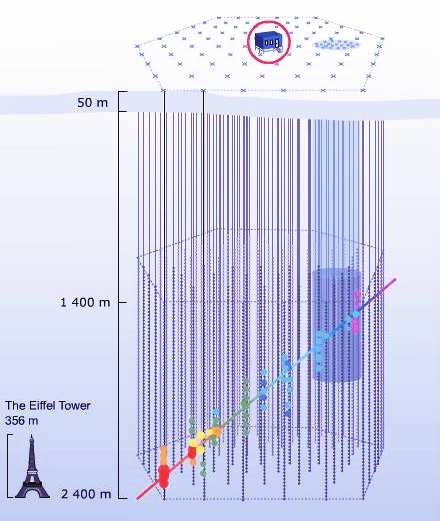
of the IceCube geometrical size refer to the ?gure III.1.

The minimal supersymmetric model generally predicts the neutralino as

Figure III.1: Schematic drawing of IceCube using Ei?el Tower as a reference

for its size. Also a particle being detected as it passes through IceCube.

a prime candidate for cold dark matter. IceCube is sensitive to cold dark

matter particles, usually refered to as Weakly Interacting Massive Particle

(WIMP) with a mass approaching TeV. IceCube o?ers numerous discovery

possibilities including being sensitive to supernova within our galaxy and

beyond. It is capable of detecting neutrinos with energies far above those

produced at accelerators.

III.2 The IceCube detector

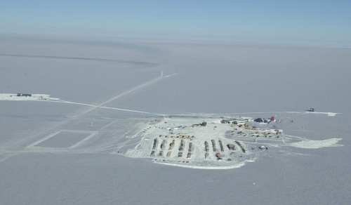
The IceCube In-Ice detector, located at the Geographic South Pole, shown in

Fig. III.2 detects high energy neutrinos that traverse the earth and interact

deep in the ice below the South Pole.

Figure III.2: IceCube Located at the South Pole, Antarctica

Particles produced by charged or neutral-current neutrino interactions

generate Cherenkov light that can be detected by an array of photomultiplier

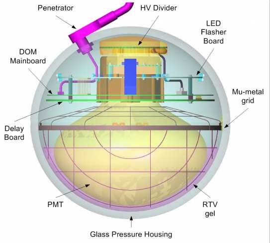
tubes (PMTs), refered to as digital optical modules (DOMs) shown in Fig.

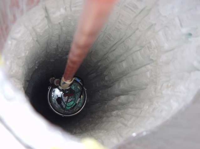
III.6. We desicrbe later in this chapter what a DOM is. Extremely deep

water ?lled holes are created by melting the ice with hot water drills and

then strings of DOMs are lowered into the water ?lled holes (see Fig. III.3).

This process will be repeated until the grid is complete. The AMANDA

detector which was completed in 2000 and has a total of 677 DOM's on

19 vertical strings served as a "proof of concept" for the IceCube detector.

IceCube is a much larger and more sophisticated detector composed of 4800

optical modules deployed on vertical strings buried 1450 to 2450 meters under

the surface containing a volume of 1km

of the ice. Each string contains 60

DOMs spaced 17 m apart.

Figure III.3: Actual DOM being deployed

III.3 IceTop

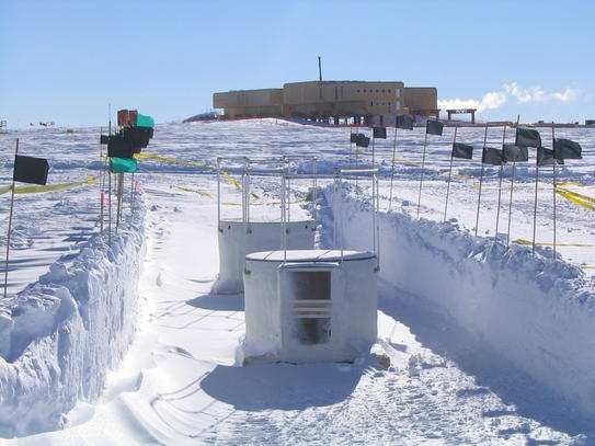
Also a surface air shower detector array, IceTop, is comprised of 320 optical

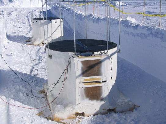
modules. The surface air-shower array is housed inside two detector tanks

each above an in-ice string. As shown in Fig. III.4 and Fig. III.5, each

2.7m diameter ice ?lled tank contains two DOMs. As well as serving as an

air-shower detector IceTop can be used to help calibrate IceCube and as a

veto for IceCube.

Figure III.4: The IceTop detector setup

The relativity sparse distribution of PMTs is ideal to IceCubs's primary

interest in having a sensitivity for neutrino energies above 1 TeV. The ?rst

string was deployed in January 2005 and 21 more in the following two austral

summers. These strings are operating well and construction is on schedule for

completion of IceCube in 2011. Each DOM, as shown in III.6, consists of a

13-inch diameter pressure vessel containing a Hamamatsu R7081-02 10-inch

diameter PMT, PMT base, high voltage supply and signal processing and

calibration electronics. The trigger and front-end electronics are located on

Figure III.5: The IceTop detector tanks

the main board. Also enclosed are two analog-to-digital converter (ADC)

systems, a precision clock and a large Field Programmable Gate Array

(FPGA) for control and communications. All communications with the

surface are through a single twisted pair shared by two DOMs. This single

pair carries power, bi-directional data and timing calibration signals.

The PMT signal is sent to a discriminator and two separate digitizer

circuits. The ?ring of the discriminator, typically set for 1/3 of a photo-

electron pulse, initiates a digitization cycle. The ?rst digitization provides

14 bits of resolution based on a switched-capacitor-array chip. The other

digitizer system detects late arriving light which has scattered in the ice.

A second board holds 12 Light Emitting Diodes (LED) that are used for

calibration. Half of the LEDs point horizontally outward while the other

Figure III.6: Schematic cross section of a DOM

half point upwards at 45 degrees.

Modeling the performance of IceCube depends crucially on a detailed

understanding of the optical properties of the ice. Data was taken by

AMANDA using various pulsed and continuous light sources. AMANDA has

mapped scattering and absorption of light to study the optical properties

of the glacial ice at the South Pole for wavelengths between 313 and 560

nm at depths between 1100 m and 2350 m [8]. As much as a factor of

seven variations for scattering in the depth range of the IceCube DOMs was

observed. A notable observation concerning the ice properties is the ice has

a very long absorption length, typically 100 m while the e?ective scattering

length is short, typically 20 m. For comparison, in water detectors such as

ANTARES the scattering lengths are long (almost 100m) and absorption

lengths are short (almost 20m) [10].

The scattering of light in the ice is strongly forward peaked so that

several scattering events are needed to substantially change the direction

of the photon. Therefore when looking at the e?ective scattering length,

(eff)

= L

=(1? < cos ? >) where L

is the mean distance between scatters

and < cos ? > is the average cosine of the angle of scatter. Qualitatively

speaking, L

(eff)

is the distance required to substantially change the direction

of the photon. It can be shown that scattering is described very well by the

single parameter, L

(eff)

for large distances compared to L

(eff)

. The light

that reaches a DOM typically do not take the shortest path to the DOM and

thus arrives delayed by a time, t

(residual)

. Fitting procedures use this time

information as well as the pulse heights. For high energy muons in AMANDA

the direction can be determined to less than two degrees and the energy to

0:4 in log

(10)

GeV

.[8]

III.4 GEANT Simulation

Graphical representation to the GEANT-3.21 simulation as a function of

depth is shown in the ?gure III.7. The ine?cient region of the IceCube

detector is represented by the apparent dip in the graph. This drop in

e?ciency is believed to be caused by "dirty" ice resulting from volcanic ash

being deposited there from an erupting volcano during the time the layer

was formed. This can be con?rmed by examining the graph around string

37 and at a depth of 2,050 m. This is consistant with the atmospheric muon

data.[9] Also shown in Fig. III.8 are the detected events from a 10 million

event simulation. The areas that contain a more concentrated number of

events simply coincide with the string of DOMs that are located there.[1]

IceCube's angular resolution for muons is approximately one degree at

high energies. Electromagnetic and hadronic showers are short, normally

10 to 20 meters. This results in inaccurate directions in AMANDA up

to 30 degree, but containment allows a better energy measurement (30%)

than for muons. Similar to AMANDA, IceCube has an energy threshold

around 100GeV. The trigger rate is approximately 80 Hz which is similar for

both IceCube and AMANDA where all events with 24 DOMs ?ring within

2.5 ?sec are recorded. This procedure yields around 10

events each year,

primarily going down muons arising from decays of ˇ's produced by cosmic

rays interactions in the atmosphere above the detector. Approximately 10

of these down-going muons are mis-reconstructed as up-going muons. The

primary physics sample of AMANDA consists of approximately 10

up-going

muons produced per year by neutrinos that traverse the earth and interact

in the ice in or near the detector. Very elaborate software is required to

reduce the muon background to an acceptable level by cutting out the poorly

Mean

ALLCHAN

32.74

0.2096E+05

¾ Geant Simulation

(average DOM settings)

SN n

p → e

n, AHA Model

DOM Number

Hits

Mean

ALLCHAN

-2923.

0.2093E+05

¾ Geant Simulation

(average DOM settings)

SN n

p → e

n, AHA Model

Depth (cm)

Hits

100

200

300

400

500

600

700

100

200

300

400

500

600

700

-40000

-20000

20000

40000

Figure III.7: These graphs represent the number of hits experienced by the

DOMs as a function of depth.

SN n

p ® e

n, AHA Model

X-axis (cm)

Y-axis (cm)

-80000

-60000

-40000

-20000

20000

40000

60000

80000

-80000

-60000

-40000

-20000

20000

40000

60000

80000

Figure III.8: Graphical representation of GEANT-3.21 10 million event

simulation.

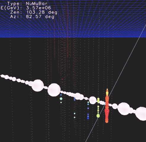
Figure III.9: Example of a muon being detected at IceCube.

reconstructed down going muons that constitute most of the background.

Atmospheric neutrinos are the majority of what is detected and provide a

very useful calibration sample for AMANDA, but also when searching for

extraterrestrial sources of neutrinos they constitute a background. The path

of a muon detected in IceCube is shown in Fig. III.9.

For the event yields and discussions presented in this analysis we assume

two things. First, the supernova occurs near the center of our galaxy,

approximately 10 kpc from earth. Second, from [12], the total energy

release in neutrinos is 3 ? 10

ergs and equally divided among the six known

neutrinos and anti-neutrinos ?avors.

CHAPTER IV

ANALYSIS AND RESULTS

IV.1 Intensity of Neutrinos from a SN

The calculations for the analysis used in this thesis are explained later

in this chapter. The following calculations were determined with the most

accurate and current values for all constants used in this thesis. We start

by calculating the binding energy of a neutron star. For a spherical mass of

uniform density the total gravitational binding self-energy U is given by the

equation :

U = ?

(IV.1)

Where G = gravitational constant, M = Mass of sphere, R = radius of the

sphere. When examining this energy in greater detail it is safe to visualize

this energy as the sum of potential energies. Therefore in order to calculate

the potential energy of a shell just on the outside of the enclosed sphere we

need to know the masses of both the shell and the sphere contained in it.

Upon determining these variables the potentials are then summed up over

the entire sphere.

First we assume a constant density ˆ, then the masses of the shell and

sphere are given:

(shell)

= 4ˇr

ˆdr

(IV.2)

(interior)

? ˇr

(IV.3)

Now taking these values and inserting them into Newtons equation for

gravitational potential energy

dU = ? G

(shell)

(interior)

(IV.4)

By integration over the volume of a sphere we get

U = ? G

(4ˇr

ˆ)(

4ˇr

)

(IV.5)

U = ? G

(IV.6)

Remember ˆ is simply equal to the mass of the whole divided by its volume

for objects with uniform densities. Therefore

ˆ =

ˇR

(IV.7)

And then ?nally plugging in the above equation,

U = ? G

(

ˇR

)

(IV.8)

U = ?

(IV.9)

U in the above equation is called the self-energy. Using the values for

G = 6:67428 ? 10

? 11

N:m

, mass of the neutron star (M

(star)

= 1:4M

(sun)

and its radius R

(star)

= 10km. The mass of the sun is equal to M

1:98892 ? 10

kg. Therefore by plugging in these values into the equation

IV.9, the binding energy of the neutron star is as follows

U = ?

G ? M

(star)

(IV.10)

U = ?

6:67428 ? 10

? 11

(1:4)

(1:98892 ? 10

)

10km

(IV.11)

U = 3:105 ? 10

(IV.12)

One Joule is equal to 6:24150974 ? 10

MeV. The binding energy is

U = 1:937921 ? 10

MeV. This value which can be divided by the number of

neutrino and antineutrino ?avors to yield the energy of E

= 3:22987 ? 10

MeV per species.

The average neutrino energy for each ?avor is given as stated in

Balantekin and Yuksel,"Neutrino mixing and nucleosynthisis in core-collapse

supernovae" [6]:

)

= 10MeV

(IV.13)

(??

)

= 15MeV

(IV.14)

;??

)

= 24MeV

(IV.15)

Now taking these energies and dividing the total energy by the energy of each

particular ?avor. The total number of neutrinos in each ?avor is computed.

)

10MeV

= 3:2299 ? 10

(IV.16)

(??

)

15MeV

= 2:1532 ? 10

(IV.17)

;??

)

24MeV

= 1:3458 ? 10

(IV.18)

With the total number of neutrinos per ?avor the intensity can be computed

using the following equation.

Intensity = I =

T otal number of neutrinos

T otal Area

(IV.19)

The area of a sphere A

sphere

= 4ˇD

, where D is the distance from the

star to earth (10kpc) contains all the neutrinos due to the exploding SN.

One parsec is equal to 3.26 light years or 3:08568025 ? 10

cm and radius

10 kpc is equal to 3:08568025 ? 10

cm. Therefore the total area covered is

sphere

= 1:195 ? 10

The ?ux for each ?avor of neutrino that would be

seen in the IceCube detector during 10 seconds can easily be calculated as

follows.

)

= 2:7134 ? 10

? 2

(IV.20)

(??

)

= 1:8094 ? 10

? 2

(IV.21)

;??

)

= 1:1309 ? 10

? 2

(IV.22)

Neutrino oscillations between SN and earth will equlize the number of each

?avor in both matter an antimatter sectors. In other words, the total average

number of electron antineutrinos used in this thesis is (2?1:1309?10

? 2

1:8094 ? 10

? 2

)=3 = 1:3571 ? 10

? 2

IV.2 Natural Abundance of Isotopes

Here we look at the natural abundance of isotopes found in the one km

ice that composes the IceCube detector. In the ice we have O

; O

; H

and H

all isotopes that make up the ice that house the IceCube detector.

Taking the density of the ice ˆ

(ice)

= 0:9167g=cm

and the mass of the ice

ice

= Volume ?ˆ

(ice)

= 0:9167 ? 10

g. This we use in determining the

mass of each molecule by multiplying the mass times the natural abundance.

)

= M

(ice)

? (0:99762) = 9:1452 ? 10

(IV.23)

)

= M

(ice)

? (0:00038) = 3:4835 ? 10

(IV.24)

)

= M

(ice)

? (0:002) = 1:833 ? 10

(IV.25)

The number of moles (N) is equal to the natural abundance divided by the

atomic mass of the molecule.

)

18:011

= 5:0776 ? 10

(IV.26)

)

19:015

= 1:832 ? 10

(IV.27)

)

20:1592

= 9:0926 ? 10

(IV.28)

The total number of molecules is the total number of moles times Avogadro's

number which is equal to N

= 6:0221415 ? 10

= N

)

= 3:0578 ? 10

(IV.29)

Table 1: Shows the di?erent isotopes and electrons found in the IceCube.

Isotope Atomic mass Natural Abundance Number of Atoms

15.995

0.99762

3:056 ? 10

16.999

0.00038

1:102 ? 10

17.9992

0.002

5:477 ? 10

1.008

0.99985

6:124 ? 10

2.014

0.0115

7:044 ? 10

0.0

3:06 ? 10

= N

)

= 1:1033 ? 10

(IV.30)

= N

)

= 5:4757 ? 10

(IV.31)

The number of molecules multiplied by two and total the sum to get

the number of Hydrogen atoms in the IceCube H

atoms

= 6:1288 ? 10

Multiplying H

atoms

by the natural abundance will yield the total number

of hydrogen isotopes in the ice. The natural abundance of H

= 99:9885%

and H

= 0:115% give the total number of atoms of H

= 6:1281 ? 10

and

= 7:0481 ? 10

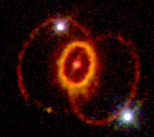
The image IV.1 is of SN 1987A, the closest SN to be observed by anyone

since SN1604.

IV.3 Cross Section Calculations

The "cross section" is the likelihood of interaction between particles in

nuclear and particle physics. If a projectile is aimed at a solid target in

Figure IV.1: SN 1987A was a supernova in the outskirts of the Tarantula

Nebula in the Large Magellanic Cloud, a nearby dwarf galaxy (ˇ 51:4 kpc).

It occurred so close to the Milky Way that it was visible to the naked eye

and it could be seen from the Southern Hemisphere. It was the closest

observed supernova since SN 1604, which occurred in the Milky Way itself.

The light from the supernova reached Earth on February 23, 1987. As the

?rst supernova discovered in 1987, it was labeled "1987A".

a speci?ed region and hits the solid target, we assume that this interaction

will occur with 100% probability. But if the projectile does not hit the solid

target, this interaction is said to have 0% probability. Therefore to compute

the total interaction probability for a single projectile to hit a solid target

will be determined by taking the ratio of the number of hits by the projectile

in the area of the solid (the cross section) to the number of hits in the total

targeted region. This basic concept to used to determine this interaction

may be extended to cases where the interaction probability in the targeted

area assumes intermediate values. These values ranging from the target itself

not being homogeneous or the interaction being mediated by a non-uniform

?eld. The di?erential cross section is de?ned as the probability to observe

a scattered particle in a given quantum state per solid angle unit within a

given cone of observation, if the target is irradiated by a ?ux of one particle

per surface unit.

The ??

p ! ne

reaction cross section is very di?cult to measure

experimentally. At low energies in the reactor energy range, the ??

have an

average energy of a few MeV [21] and are much lower in energy than the SN

neutrinos. At pion factory such as the old factories where pions are copiously

produced such as the old Los Alamos Meson Physics Facilty (LAMPF), the

's can only be the product of the ˇ

decay that are captured in the target

when they come to rest. This will make it virtually impossible to measure

this cross section. We, therefore, have to rely solely on calculations for the

above cross section.

, MeV

10 16*

Naive

0:02 0:08 0:21 0:33 1:32 5:28

Naive +

0:02 0:07 0:19 0:29 1:16 4:64

Vogel and Beacom

0:12 0:07 0:19 0:29 0:98 2:31

4 Strumia and Vissani

0:12 0:07 0:19 0:29 0:98 3:17

Horowitz

0:022 0:09 0:24 0:33 1:12 3:3

Llewellyn-Smith+

0:012 0:07 0:19 0:29 1:04 3:22

LS + VB

0:012 0:07 0:19 0:29 1:04 3:22

8 Gaisser and O'Connell 0:03 0:12 0:31 0:48 1:92 7:68

Table 2: Various approximations for ˙(??

p ! ne?) in units of 10

? 40

represents SN neutrino energy.

Table 2 shows the cross section calculation from di?erent authors. In

the following calculations we de?ne ? = m

? m

ˇ 1:293 MeV and M =

+ m

)=2 ˇ 938:9 MeV. In the table we consider the ??

reaction.

1. The naive low-energy approximation (see e.g.[18])

˙ ˇ 9:52 ? 10

? 44

MeV

;

= E

? ? for ??

and ?

; (IV.32)

obtained by normalizing the leading-order (LO) result to the neutron

lifetime, overestimates ˙(??

p) especially at high energy.

2. A simple approximation which agrees with our full result within a few

per-million for E

? 300 MeV is

˙(??

p) ˇ 10

? 43

? 0:07056+0:02018 ln E

? 0:001953 ln

; (IV.33)

= E

? ?

(IV.34)

where all energies are expressed in MeV.

3. The low-energy approximation of Vogel and Beacom [16] (which

include ?rst order corrections in " = E

, given only for anti-

neutrinos) is very accurate at low energies (E

< 60 MeV), however

underestimates the number of supernova IBD neutrino events at highest

energies by 10%. Higher order terms in " happen to be dominant

already at E

> 135 MeV, where the expansion breaks down giving a

negative cross-section [16, 19].

4. The Strumia and Vissani[13] low-energy approximation, de?ned by

the equation:

A ' M

? g

)(t ? m

) ? M

+ g

) ? 2m

M?g

+ f

)

B ' t g

+ f

)

C ' (f

+ g

)=4

(IV.35)

can be used from low energies up to the energies relevant for supernova

detection. They expand the squared amplitude in " but, unlike Vogel

and Beacom, they treat kinematics exactly, so that some higher order

terms are included in the Strumia and Vissani cross section. In above

equations, M is the average mass of a neutron-proton pair, f

= 1 is

the vector coupling constant, f

= 3:71f

=2M, g

= 1:272 ? :002 is the

axial vector coupling constant, and t = m

? m

? 2m

? E

5. The high-energy approximation of Horowitz [19], obtained from the

Llewellyn-Smith formulae[14] setting m

= 0, was not tailored to be

used below ˘ 10 MeV, and it is not precise in the region relevant for

supernova neutrino detection; however, it is presumably adequate to

describe supernova neutrino transport.

6. The Llewellyn-Smith high-energy approximation, improved adding

6=m

in s; t; u, but not in M is very accurate at all energies relevant

for supernova neutrinos, failing only at the lowest energies. As proved

previously, this is a consequence of the absence in jM

j of corrections

of order ?=m

7. Approximation 6. can be improved by including also the dominant low-

energy e?ects in the amplitude M, as discussed in section IIB of [16].

8. The Gaisser and O'Connell formalisim was used to produce the

results shown in ?gure IV.2.

In this ?gure, we show the distribution of the di?erent neutrino

concentrations within the neutrinosphere. The emitted positrons after

intercation in the IceCube was generated with the formalisim of Gaisser

and O'Connell[2]. Also shown for comparison are the data form the

detected events of IMB and Kamioka for SN1987A.

IV.4 Detector Sensitivity to SN Explosion

The intensity times the inverse ?-decay cross section (0:31 ? 10

? 40

)

and the number of protons (6:13 ? 10

) yields the number of positrons

generated in the detector which is N

= 2:60 ? 10

. A GEANT-3.21

calculation [20] with the IceCube geometry and the DOM quantum

e?ciency with layered ice yields an e?ciency of 0:0075 for production

of photoelectrons (PE). This gives 1:95 ? 10

DOM hits in a 10-second

interval. To obtain the total noise for the same 10-second time interval

+ p

+ n Scattering

Mean

ALLCHAN

16.07

1.0000

Energy Distribution of Electron Neutrinos (MeV)

Counts

Mean

ALLCHAN

22.05

20.00

. SN87A from IMB and Kamioka

¾ MC

Energy Distribution of Positrons (MeV)

Counts

Mean

ALLCHAN

0.3892E-01

0.2458E-01

Cosine of the angle of the positrons

Counts

0.02

0.04

100

0.05

0.1

0.15

x 10

-2

100

0.2

0.4

x 10

-3

-1

-0.8

-0.6

-0.4

-0.2

0.2

0.4

0.6

0.8

Figure IV.2: Comparison of the energy distribution of the Supernova Electron

Neutrinos that of the Positrons during ??

+ p ! e

+ n scattering in MeV.[1]

of all 4800 DOMs, we multiply number of DOMs by the time ?t = 10

sec and the dark rate of 300 Hz, Therefore,

DetectorNoise = 4800 ? 300 ? 10 = 1:44 ? 10

(IV.36)

This value gives rise to a statistical ?uctuation of ˙ equal to ?3800. In

turn yields a value of 513˙ that when divided by 5:5˙ (IceCube trigger)

is 93. Solving the equation below gives the distance that the detector

will be sensitive to

100

= 93

(IV.37)

= 9300

(IV.38)

R = 97kpc:

(IV.39)

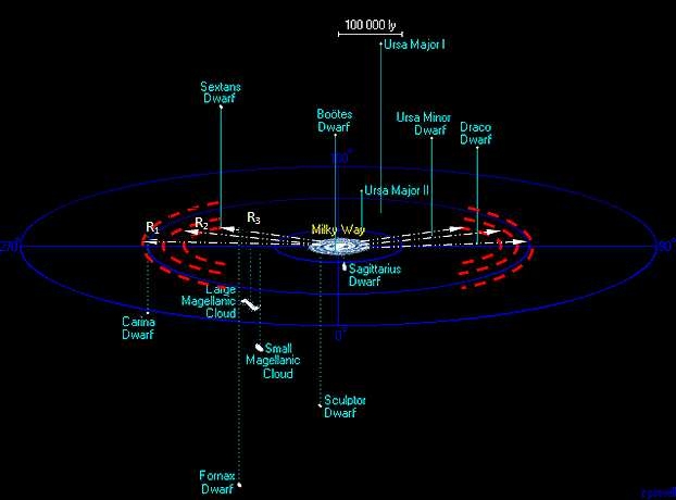
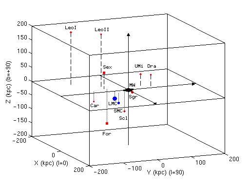
In the ?gures IV.3,IV.4, we show the range of sensitivity for the IceCube

detector using the values shown in the table 3. The ?gure IV.5 shows a 3-D

representation of the Milky Way along with its nearest neighboring galaxies.

Figure IV.3: Schematic view showing the range of the sensitivity of the

IceCube detector along with corresponding authors calculations of sensitivity

in our galactic neighborhood. The values for the corresponding radius are

= 97 kps, R

= 86 kpc, and R

= 76 kpc, corresponding to cross sections

from Gaisser and O'Connell, Horowitz, and (Naive +, Vogel and Beacom,

Srumia and Vissani, Llewellyn-Smith +, and LS+VB), respectively. Each

shown radius can be visualized as having an spherical shape surrounding the

galactic neighborhood. Not shown in the above picture is the Naive model

that yields a sensitive radius of 79 kpc.[22]

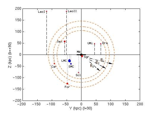
Figure IV.4: Schematic top view showing the range of sensitivity of the

IceCube detector along with the same corresponding values for R

, R

, and

as stated in the previous ?gure IV.3.[23]

Figure IV.5: 3-D view of Milky Way and neighboring galaxies.[23]

Table 3: Sensitivity of detection with di?erent authors' calculations

Author

˙(??

p ! ne

) Distance (kpc)

Naive

BIBLIOGRAPHY

[1] These GEANT calculations were performed by Ali R. Fazely.
[2] T.K. Gaisser and J.S. O'Connell, Interactions of atmospheric neutrinos
on nuclei at low energy, Phys. Rev. D 34 3 p822 (1986)
[3] M. Liebendorfer, et al., Phys. Rev. D 63 103004 (2001)
[4] Amol S. Dighe, Mathis Th. Keil and Georg G Ra?elt, hep-ph/0303210v3
(2003), JCAP 0306, 005 (2003).
[5] W. Pauli, Letter to the Physical Institute of the Federal Institute of
Technology (ETH), unpublished, (December 1930)
[6] A. B. Balantekin and H. Yuksel, New Journal of Physics 7 (2005)
[7] V. Barger, D. Marfatia and B.P. Wood, arXiv:hep-ph/0112125v3 (2002),
Phys. Lett. B547, 37-42 (2002).
[8] M. Ackermann et al., J of Geophys. Res. v111, D13203 (2006).
[9] http : ==wiki:icecube:wisc:edu=index:php=GEANT=IceSim
c
omparison
[10] V. Flaminio, ANTARES Collaboration, Proc Sci. HEP2005 (2006) 25
[11] R. Buras, H-T Janka, arXiv:astro-ph/0205006v1 (2002),Astrophys.J.
587, 320-326 (2003.
[12] Kate Scholberg, arXiv:hep-ex/0008044v1 (2000), Nucl. Phys. Proc.
Suppl. 91, 331-337 (2000).
[13] A. Strumia and F. Vissani, arXiv:astro-ph/0302055 v2 (29 Apr 2003),
Phys.Lett. B564, 42-54 (2003).
[14] C.H. Llewellyn-Smith, Phys. Rep. 3 261 (1972).
[15] Suzuki H 1993 Proc. Int. Symp. on Neutrino Astrophysics ed Y suzuki
and K. Nakamura (Tokyo: Universal Acadamy Press)
[16] P. Vogel and J.F. Beacom, Angular distribution of neutron inverse beta
decay, nubar
e
+ p ! (e
+
) + n,The American Physical Society (1999)
[17] H.M. Gallagher and M.C. Goodman, Neutrino Cross Sections, NuMI-
112 PDK-626 (Nov. 10, 1995)
43
44
[18] C. Bemporad, G. Gratta and P. Vogel, Rev. Mod. Phys. 74 (2002) 297
[19] C.J. Horowitz, Phys. Rev. D 65 (2002) 043001.
[20] A. R. Fazely, Private Communications, (2008)
[21] H. Murayama and A. Pierce, arXiv:hep-ph/0012075v3 (2000), Phys.Rev.
D65, 013012 (2002).
[22] http://www.astro.uu.se/ ns/mwsat.html
[23] http://www.atlasoftheuniverse.com/sattelit.html
VITA
Aaron Simon Richard was born in Baton Rouge, capitol city of Louisiana,
on the 2nd day of September in 1969. He graduated from McKinley Senior
High School in 1987. Upon completing requirements for Bachelor of Science
in Physics he was awarded his degree in May of 1995. After a short leave,
he was admitted to the Master of Science program at Southern University in
1999 to pursue his career in Physics.
45
APPROVAL FOR SCHOLARLY DISSEMINATION
The author grants to the Souther University Library the right to
reproduce, by the appropriate methods, upon request, any or all portions
of this thesis.
It is understood that "request" consists of an agreement on the part of
the requesting party, that said reproduction will not occur without written
approval of the author of this thesis.
The author of this thesis reserves the right to publish freely, in the
literature, at any time, any or all the portions of this thesis.