UPTEC ES07 030

Examensarbete 20 p

December 2007

Designing an H-rotor type Wind

Turbine for Operation on

Amundsen-Scott South Pole Station

Mats Wahl

Teknisk- naturvetenskaplig fakultet

UTH-enheten

Besöksadress:

Ångströmlaboratoriet

Lägerhyddsvägen 1

Hus 4, Plan 0

Postadress:

Box 536

751 21 Uppsala

Telefon:

018 – 471 30 03

Telefax:

018 – 471 30 00

Hemsida:

http://www.teknat.uu.se/student

Abstract

Designing an H-rotor type Wind Turbine for

Operation on Amundsen-Scott South Pole Station

Mats Wahl

This thesis focuses on designing the turbine, tower structure and generator for an

H-rotor type wind turbine. The produced power will be used for heating of drilling

equipment, stored in containers, on the Amundsen-Scott South Pole Station. A 23

kW wind turbine producing 5 kW on average has been designed. Moreover, the

design has been tested to be mounted on top of the container storing the drilling

equipment. Climatological data have been processed to describe the wind regime in

useful terms. A three bladed H-rotor has been dimensioned for the mean power

demand using a Conformal Mapping and Double Multiple Streamtube model. The

tower structure has been tested considering strength and eigenfrequencies with

simulations based on Finite Element Method and analytical calculations. An outer

rotor generator has been designed using a simulation code based on Finite Element

Method. The site specific constraints due to the extreme climate in Antarctica are

considered throughout the design process. Installing this wind turbine would be a first

step towards higher penetration of renewable energy sources on the Amundsen-Scott

South Pole Station.

ISSN: 1650-8300, UPTEC ES07 030

Examinator: Ulla Tengblad

Ämnesgranskare: Hans Bernhoff

Handledare: Paul Deglaire

Sammanfattning

Detta projekt syftar till att öka andelen förnyelsebar el-generering vid den amerikanska polar-

forskningsstationen Amundsen-Scott på sydpolen. Projektet har startats på initiativ av Svenska

Polarforskningssekretariatet i samarbete med det internationella forskningsprojektet ICECUBE

samt Stockholms universitet och Uppsala universitet. Det övergripande syftet är att undersöka

möjligheten till ett vindkraftsbaserat kraftförsörjningssystem.

Ett vindkraftverk har designats för de specifika förhållanden som råder vid sydpolen. Det koncept

som arbetats fram utgörs av en vertikalaxlad vindturbin, en så kallad H-rotor, och en direktdriven

generator. En prototyp av liknande karaktär har konstruerats vid avdelningen för Elektricitetslära

och Åskforskning, Uppsala Universitet, vid vilken handledaren för projektet är verksam.

Projektets syfte är att designa ett vindkraftverk vilket har en medeleffekt på 5 kW för de vind-

förhållanden som råder vid Sydpolen.

Klimatologiska data har bearbetats och vindförhållandena på plats har formulerats i användbara

termer. Ur detta har det visats att vindresurserna på sydpolen är tillräckliga för att introducera ett

vindkraftsbaserat kraftförsörjningssystem. En frekvensdistribution för vindhastigheten har tagits

fram och denna har implementerats i effekt- respektive energiberäkningar.

En för H-rotorer speciellt framtagen modell har använts vid simuleringar för att optimera

turbinens utformning. En designstrategi har utarbetats för att på ett så effektivt sätt som möjligt

optimera turbinen med hänsyn till soliditet, bladprofil, infästningsvinkel samt infästningspunkt

(mellan rotorns blad och bärarmar). Den tillämpade designstrategin ger möjlighet att skala

turbinen efter önskat effektbehov.

Fundamentet utgörs av två ihopsatta containrar. Den främsta anledningen till varför vindkraft-

verket ska monteras ovanpå två containrar är att dessa kontrolleras av ICECUBE projektet. På

grund av detta krävs väsentligt färre tillstånd än ett fundament som byggs i eller ovanpå snön. För

att utvärdera huruvida denna typ av fundament är tillämpbart har lasterna på både turbin och

övrig struktur uppskattats varefter stabilitetsberäkningar utförts.

Ett fackverkstorn har dimensionerats för att möta kraven på en tillräckligt stark och styv struktur.

Det främsta designkriteriet är att tornets egenfrekvens inte sammanfaller med turbinens drift-

frekvens eller någon av dess övertoner. Detta för att strukturen inte får komma i självsvängning

med stora deformationer som följd. Spännings- och frekvensanalyser har utförts med hjälp av

COMSOL Multiphysics som är ett simuleringsprogram baserat på finita elementmetoder. Vidare

har

simuleringar och analytiska beräkningar genomförts för att verifiera att det inte föreligger problem

med maximala spänningar, elastisk instabilitet eller utmattning hos de enskilda fackverks-

medlemmarna.

En direktdriven generator har dimensionerats med hjälp av simuleringar med finita elementmetoder

för elektromagnetiska applikationer. Att generatorn är direktdriven innebär att turbinens roterande

rörelse överförs till generatorn utan att växlas upp. Generatorn har fler elektriska poler för att

generera elektricitet med tillräckligt hög frekvens. Polerna utgörs av permanentmagneter. Turbinens

bärarmar är länkade direkt till generatorns utanpåliggande rotor. En sådan design medför att vind-

kraftverket enbart har en rörlig del.

Då turbinen designad för att möta kravet på en medeleffekt på 5 kW visade sig vara relativt stor

har två alternativa koncept arbetats fram. En turbin för medeleffekt på 2.5 kW och en på 1.0 kW

har dimensionerats. Genom att installera 2 respektive 5 av dessa uppfylls effektkravet. Detta har

medfört att tre tornstrukturer samt tre generatorer har designats.

En kostnadsuppskattning för de tre koncepten har utförts baserat på tidigare prototypprojekt samt

specifika materialkostnader. Delvis mot bakgrund av den totala systemkostnaden har konceptet

baserat på en stor turbin föreslagits för fortsatt utredning.

Projektet har resulterat i en föreslagen 23 kW turbin kopplad till en direktdriven generator placerad

i navet med utanpåliggande rotor. Navhöjden är 10m. Turbinen har tre blad, radien är 5 m och

bladlängden är 10 m. Symmetriska NACA 0018 profiler används med en kordlängd på 0.45 m. Detta

ger en soliditet på 0.27. Turbinen är optimerad för ett löptal på 4 med ett förväntat maximalt C

på 0.38.

Contents

1 Introduction

1.1 Background . . . . . . . . . . . . . . . . . . . . . . . . . . . . . . . . . . . . . . . . 1

1.1.1 Antarctica and Amundsen Scott South Pole Station . . . . . . . . . . . . . 1

1.1.2 The Swedish Polar Research Secretariat . . . . . . . . . . . . . . . . . . . . 2

1.1.3 The IceCube project and purpose of wind power installation . . . . . . . . 2

1.1.4 Expectations on the project . . . . . . . . . . . . . . . . . . . . . . . . . . . 2

1.2 Aim of the project . . . . . . . . . . . . . . . . . . . . . . . . . . . . . . . . . . . . 2

1.3 The overall design strategy . . . . . . . . . . . . . . . . . . . . . . . . . . . . . . . 3

1.4 Wind power . . . . . . . . . . . . . . . . . . . . . . . . . . . . . . . . . . . . . . . . 3

1.5 Site specific demands . . . . . . . . . . . . . . . . . . . . . . . . . . . . . . . . . . . 4

1.5.1 Wind power operation in cold climate . . . . . . . . . . . . . . . . . . . . . 4

1.5.2 The overall design . . . . . . . . . . . . . . . . . . . . . . . . . . . . . . . . 5

1.6 Theory . . . . . . . . . . . . . . . . . . . . . . . . . . . . . . . . . . . . . . . . . . . 5

1.6.1 Finite Element Method . . . . . . . . . . . . . . . . . . . . . . . . . . . . . 5

2 Designing of the turbine

2.1 Introduction . . . . . . . . . . . . . . . . . . . . . . . . . . . . . . . . . . . . . . . . 7

2.1.1 The chosen wind turbine concept . . . . . . . . . . . . . . . . . . . . . . . . 7

2.2 Design strategy . . . . . . . . . . . . . . . . . . . . . . . . . . . . . . . . . . . . . . 8

2.3 Wind resources . . . . . . . . . . . . . . . . . . . . . . . . . . . . . . . . . . . . . . 9

2.3.1 Data resources . . . . . . . . . . . . . . . . . . . . . . . . . . . . . . . . . . 9

2.3.2 Treatment of data . . . . . . . . . . . . . . . . . . . . . . . . . . . . . . . . 9

2.3.3 Mean wind speed . . . . . . . . . . . . . . . . . . . . . . . . . . . . . . . . . 10

2.3.4 Wind speed frequency distribution . . . . . . . . . . . . . . . . . . . . . . . 10

2.3.5 The design wind speed . . . . . . . . . . . . . . . . . . . . . . . . . . . . . . 11

2.3.6 Density of the air . . . . . . . . . . . . . . . . . . . . . . . . . . . . . . . . . 11

2.4 Objective function . . . . . . . . . . . . . . . . . . . . . . . . . . . . . . . . . . . . 11

2.5 Design parameters . . . . . . . . . . . . . . . . . . . . . . . . . . . . . . . . . . . . 11

2.5.1 Fixed parameters . . . . . . . . . . . . . . . . . . . . . . . . . . . . . . . . . 12

2.6 Estimation of a tentative design . . . . . . . . . . . . . . . . . . . . . . . . . . . . . 12

2.7 Optimizing the tentative design using a CMDMS model . . . . . . . . . . . . . . . 13

2.7.1 The CMDMS model . . . . . . . . . . . . . . . . . . . . . . . . . . . . . . . 13

2.7.2 Problem finding input data . . . . . . . . . . . . . . . . . . . . . . . . . . . 14

2.8 Designing of one 5 kW turbine . . . . . . . . . . . . . . . . . . . . . . . . . . . . . 15

2.8.1 The reference design . . . . . . . . . . . . . . . . . . . . . . . . . . . . . . . 15

2.8.2 Optimizing the solidity . . . . . . . . . . . . . . . . . . . . . . . . . . . . . 15

2.8.3 Optimizing the blade profile thickness . . . . . . . . . . . . . . . . . . . . . 17

2.8.4 Optimizing the fixed blade pitch . . . . . . . . . . . . . . . . . . . . . . . . 18

2.8.5 Optimizing the point of attachment . . . . . . . . . . . . . . . . . . . . . . 20

2.8.6 Control strategy . . . . . . . . . . . . . . . . . . . . . . . . . . . . . . . . . 22

2.9 The proposed 5 kW design . . . . . . . . . . . . . . . . . . . . . . . . . . . . . . . . 22

2.10 Alternative number of turbines, two 2.5 kW, five 1 kW . . . . . . . . . . . . . . . . 23

3 Load estimates and stability calculations on the foundation

3.1 Introduction . . . . . . . . . . . . . . . . . . . . . . . . . . . . . . . . . . . . . . . . 27

3.2 Simulation tool used in the structural mechanic analysis . . . . . . . . . . . . . . . 27

3.3 Load estimates . . . . . . . . . . . . . . . . . . . . . . . . . . . . . . . . . . . . . . 28

3.3.1 Weight loads . . . . . . . . . . . . . . . . . . . . . . . . . . . . . . . . . . . 28

3.3.2 Static pressure forces and torques due to the wind . . . . . . . . . . . . . . 28

3.3.3 Unsteady loads . . . . . . . . . . . . . . . . . . . . . . . . . . . . . . . . . . 30

3.4 Constraints and calculations . . . . . . . . . . . . . . . . . . . . . . . . . . . . . . . 32

3.4.1 Overturning . . . . . . . . . . . . . . . . . . . . . . . . . . . . . . . . . . . . 32

3.4.2 Container strength . . . . . . . . . . . . . . . . . . . . . . . . . . . . . . . . 33

3.4.3 Snow collapse and settlement . . . . . . . . . . . . . . . . . . . . . . . . . . 33

3.4.4 Drift of the structure . . . . . . . . . . . . . . . . . . . . . . . . . . . . . . . 34

3.4.5 Eigenfrequency . . . . . . . . . . . . . . . . . . . . . . . . . . . . . . . . . . 34

3.5 Discussion . . . . . . . . . . . . . . . . . . . . . . . . . . . . . . . . . . . . . . . . . 35

3.5.1 Overturning . . . . . . . . . . . . . . . . . . . . . . . . . . . . . . . . . . . . 35

3.5.2 Container strength . . . . . . . . . . . . . . . . . . . . . . . . . . . . . . . . 35

3.5.3 Drift of the container foundation . . . . . . . . . . . . . . . . . . . . . . . . 35

3.5.4 Snow collapse and settlement . . . . . . . . . . . . . . . . . . . . . . . . . . 36

3.5.5 Eigenfrequency . . . . . . . . . . . . . . . . . . . . . . . . . . . . . . . . . . 36

4 Designing of the tower structure

4.1 Introduction . . . . . . . . . . . . . . . . . . . . . . . . . . . . . . . . . . . . . . . . 37

4.2 Design strategy . . . . . . . . . . . . . . . . . . . . . . . . . . . . . . . . . . . . . . 37

4.3 Objective function . . . . . . . . . . . . . . . . . . . . . . . . . . . . . . . . . . . . 37

4.4 Constraints . . . . . . . . . . . . . . . . . . . . . . . . . . . . . . . . . . . . . . . . 38

4.4.1 Dimensions . . . . . . . . . . . . . . . . . . . . . . . . . . . . . . . . . . . . 38

4.4.2 Eigenfrequencies . . . . . . . . . . . . . . . . . . . . . . . . . . . . . . . . . 38

4.4.3 Elastic limit . . . . . . . . . . . . . . . . . . . . . . . . . . . . . . . . . . . . 38

4.4.4 Elastic instability . . . . . . . . . . . . . . . . . . . . . . . . . . . . . . . . . 38

4.4.5 Fatigue . . . . . . . . . . . . . . . . . . . . . . . . . . . . . . . . . . . . . . 38

4.4.6 Displacement . . . . . . . . . . . . . . . . . . . . . . . . . . . . . . . . . . . 38

4.4.7 Ease of transportation, installation and maintenance . . . . . . . . . . . . . 39

4.5 Design parameters . . . . . . . . . . . . . . . . . . . . . . . . . . . . . . . . . . . . 39

4.5.1 Fixed parameters . . . . . . . . . . . . . . . . . . . . . . . . . . . . . . . . . 39

4.6 Optimizating the tower structure using COMSOL . . . . . . . . . . . . . . . . . . . 39

4.7 Material chosen . . . . . . . . . . . . . . . . . . . . . . . . . . . . . . . . . . . . . . 40

4.8 The proposed tower structure designs . . . . . . . . . . . . . . . . . . . . . . . . . 41

4.9 Verification of the design constraints . . . . . . . . . . . . . . . . . . . . . . . . . . 41

4.9.1 Eigenfrequency simulation . . . . . . . . . . . . . . . . . . . . . . . . . . . . 41

4.9.2 Stresses and displacements simulations . . . . . . . . . . . . . . . . . . . . . 42

4.9.3 Elastic instability calculations . . . . . . . . . . . . . . . . . . . . . . . . . . 43

4.9.4 Fatigue calculations . . . . . . . . . . . . . . . . . . . . . . . . . . . . . . . 44

4.10 Discussion . . . . . . . . . . . . . . . . . . . . . . . . . . . . . . . . . . . . . . . . . 44

4.10.1 Eigenfrequencies . . . . . . . . . . . . . . . . . . . . . . . . . . . . . . . . . 44

4.10.2 Stresses and displacement . . . . . . . . . . . . . . . . . . . . . . . . . . . . 45

4.10.3 Elastic instability . . . . . . . . . . . . . . . . . . . . . . . . . . . . . . . . . 45

4.10.4 Fatigue . . . . . . . . . . . . . . . . . . . . . . . . . . . . . . . . . . . . . . 45

5 Designing of the generator

5.1 Introduction . . . . . . . . . . . . . . . . . . . . . . . . . . . . . . . . . . . . . . . . 48

iii

5.1.1 Direct drive concept . . . . . . . . . . . . . . . . . . . . . . . . . . . . . . . 48

5.1.2 Synchronous permanent magnet generator . . . . . . . . . . . . . . . . . . . 48

5.1.3 Generator losses . . . . . . . . . . . . . . . . . . . . . . . . . . . . . . . . . 48

5.2 Simulation tool used in the electromagnetic analysis . . . . . . . . . . . . . . . . . 50

5.3 Design strategy . . . . . . . . . . . . . . . . . . . . . . . . . . . . . . . . . . . . . . 51

5.4 Objective function . . . . . . . . . . . . . . . . . . . . . . . . . . . . . . . . . . . . 51

5.5 Design parameters . . . . . . . . . . . . . . . . . . . . . . . . . . . . . . . . . . . . 52

5.5.1 Fixed parameters . . . . . . . . . . . . . . . . . . . . . . . . . . . . . . . . . 52

5.6 Optimizing the generator using ACE . . . . . . . . . . . . . . . . . . . . . . . . . . 53

5.7 Estimating the electric efficiency when operating at part load . . . . . . . . . . . . 54

5.8 The proposed generator designs . . . . . . . . . . . . . . . . . . . . . . . . . . . . . 55

5.9 Discussion . . . . . . . . . . . . . . . . . . . . . . . . . . . . . . . . . . . . . . . . . 56

6 Conclusions

6.1 Cost estimates . . . . . . . . . . . . . . . . . . . . . . . . . . . . . . . . . . . . . . 57

6.2 Comparison between the different wind turbine concepts . . . . . . . . . . . . . . . 58

6.3 Choice of turbine concept . . . . . . . . . . . . . . . . . . . . . . . . . . . . . . . . 58

6.4 Recommendations for future work . . . . . . . . . . . . . . . . . . . . . . . . . . . 59

6.5 Recommendations to future designers of H-rotors . . . . . . . . . . . . . . . . . . . 60

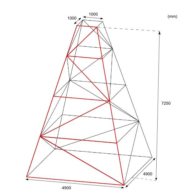
A Sketch of the truss tower

Chapter 1

Introduction

1.1 Background

1.1.1 Antarctica and Amundsen Scott South Pole Station

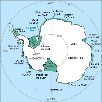
On average, Antarctica is the coldest, driest, windiest and highest elevated of all the continents

[1]. Since there is little precipitation, except along the coastlines, the interior plateau is techni-

cally the largest desert in the world. The continent makes up about 10% of the land surface on

Earth. Antarctica has six month of daylight and six months of darkness. The continent lies within

the Antarctic Circle (66

south of the equator), except the northern part of the Antarctic

Peninsula.

Figure 1.1: Antarctica.

Americans have occupied the South Pole continuously since November 1956. The first station,

built in 1956-1957, was constructed to support researchers during the International Geophysical

Year between 1957 and 1958. The station has evolved and new buildings have been constructed as

interest in polar research through the years has increased. The latest construction will be finished

in 2007 and enables up to 150 people to work there during the austral summers. The name of the

station honors Roald Amundsen who reached the South Pole in 1911, and Robert F. Scott who

accomplished the same heroic feat in 1912 [2].

1.1.2 The Swedish Polar Research Secretariat

The Swedish Polar Research Secretariat [3] is the initiator of this Master Science Project. The

main task of the Swedish Polar Research Secretariat is to promote and co-ordinate Swedish Polar

research. This means planning research and development and organizing expeditions to the Arctic

and Antarctic regions.

1.1.3 The IceCube project and purpose of wind power installation

The ICECUBE project is an international particle physics program which currently is building a

neutrino telescope in connection to Amundsen Scott South Pole Station. The telescope will be

buried 1.4 to 2.4 kilometers below the surface of the ice and will be constructed during the austral

summers over the next four years [4].

Today the Amundsen Scott station is powered by combustion engines. These consume large

amounts of energy, especially if the fuel consumption caused by transportation to the South Pole is

taken into account. This means not only pollution of the atmosphere in Antarctica but also a very

high cost of energy. Based on these two incentives, IceCube plan to be the first project introducing

wind power at the Amundsen Scott station.

1.1.4 Expectations on the project

The request from the IceCube project is to design a wind turbine producing between 26 and

43MWh per year. This result in a mean power output of 3-5 kW over the year at the root mean

cube

wind speed of 6.7 m/s at this site. The electrical power produced will be used to heat drilling

equipment stored in containers at the station. This project is a first step toward higher penetration

of wind power in the existing electrical grid at the station.

1.2 Aim of the project

Based on the expectations from ICECUBE the aim of this project is to design an H-rotor type

wind turbine producing 5 kW in 6.7 m/s. The wind turbine includes turbine, tower structure and

generator. Moreover, the total cost of the wind turbine will be estimated.

The site specific constraints due to the harsh climate in Antarctica limit the number of suitable

wind turbines available on the market. This motivates the designing of a wind turbine well adapted

for the climate on South Pole. The choice of designing an H-rotor type wind turbine is also due to

the extensive material that already can be found concerning suitable horizontal axis wind turbine

concepts for the Antarctic region [5][6]. Setting the mean power as design criteria is unusual in

wind power industry. Usually the rated wind speeds are in the range of 12 m/s. The reader should

have this in mind when comparing the 5 kW turbine in this report with conventional wind turbines

on the market.

The root mean cube wind speed is often used as design wind speed for wind turbine applications.

1.3 The overall design strategy

The first step is to describe the wind regime in useful terms. Climatological data has been gathered

and from these the wind speed distribution is derived. Based on the wind regime a turbine is

designed to meet the request of 5 kW mean power output. This is performed utilizing a simulation

tool especially coded for simulating on the type of wind turbine designed.

The foundation in this application is not free to design. Because of this, the next step is to

validate the stability of the foundation during both hurricane conditions and operation. This is

performed based on load estimates using the turbine design and approximate designs of the tower

and generator. The structural mechanic analysis is performed using a simulation tool based on

finite element methods.

The tower structure is designed to not have any eigenfrequencies interfering with the turbines

operational frequency. This and the choice of material (due to the low temperatures) set the

primary design criteria.

The last part to design is the generator. The generator is designed to minimize the losses when

operated at part load as this represent the most common load case for this wind turbine. This is

performed utilizing a Finite Element Method simulation especially developed for simulating this

type of generator.

1.4 Wind power

A wind turbine is a machine that converts the kinetic energy in wind into mechanical energy. The

mechanical energy is directly converted into electricity. The turbine concept is often named after

the axis of rotation for the turbine. A horizontal axis wind turbine (HAWT) has an horizontal shaft

(see figure 1.2(a)). A vertical axis wind turbine (VAWT) has a vertical shaft (see figure 1.2(b)).

For a more extensive comparison between the two different wind turbine concepts see reference [7].

(a) HAWT.

(b) VAWT.

Figure 1.2: Visual comparison between the two major wind turbine concepts denoted by the axis of

rotation.

The amount of power P that can be absorbed in a wind turbine is described by equation 1.1

P =1

ˆAC

(1.1)

where ˆ is the air density, A is the swept area of the turbine, C

is aerodynamic efficiency (denoted

power coefficient) and U is the free wind speed.

1.5 Site specific demands

1.5.1 Wind power operation in cold climate

There are several aspects to be considered when planning for wind turbine operation in cold climate

areas. The specific constraints are due to icing, material properties at low temperatures and snow

drift. To strive for minimum maintenance the design should be adapted to cold climate application.

Icing

Icing is the most prominent problem associated with operation in cold climate. Icing occurs when

the temperature is below 0? and there is humidity in the air. Ice accumulation on any of the

turbine’s aerodynamic parts degrades the performance. Depending on the wind turbine design and

regulation method the effects from ice accumulation on the blades are different [8]. As described in

section 1.1.1 the Antarctic plateau is one of the largest deserts on earth in means of low humidity.

Icing is a function of both temperature and humidity. That is why icing is not necessarily a problem

in very cold areas. In fact, the air at the South Pole is so dry all year round that the risk of icing

can be neglected.

Low temperatures

Operation in low temperatures put constraints on the choice of materials in all of the wind turbine

parts [8]. The material properties are changing with temperature. Glass fiber structures, plastics,

rubber and metals may all suffer from being brittle at low temperatures. Metals in general become

more fragile and less resistant to fatigue. Cold resistant steel is always recommended. Cables,

for which the plastic insulation becomes brittle, may fracture and lead to shorting. Standard

oils and lubricants become more viscous in low temperatures. This may lead to higher loads on

hydraulic systems, gearboxes and bearings. Use of synthetic lubricants rated for low temperatures

are recommended. All parts of the wind turbine that are not directly modified for use in cold

climate but still may suffer from the harsh conditions have to be heated. Examples are gearboxes,

generators, yawing mechanisms and electronics.

Snow

Snow is easily suspended and transported by the wind. The mass flux per volume of snow in the

air has been estimated to the sixth power of the wind speed and to vary linearly with the height.

Snow ingress is the most prominent problem related to blowing snow in wind turbine application[9].

Designing a structure with a minimum of entries for the snow particles is the easiest way of reducing

the problem. Careful choice in sealing- or filter method is recommended where any type of opening

is needed.

Special concerns about installation and maintenance

Wind turbines for cold climate operation are often installed in remote areas. A minimum of

maintenance is particularly important when the replacement of broken parts can take several

months. A simple design is preferable in order to minimize the amount of parts that can break.

To ease the installation and transport, a design that can be assembled on site is preferable. Building

a foundation on the snow is not trivial. Use of existing towers or buildings should be considered.

An additional problem related to building the foundation in or on top of the snow layer is the

snow drift. In Antarctic regions snow can rapidly cover man made structures and reduce the useful

tower height [9].

1.5.2 The overall design

The overall design has to be well suited for cold climate application. One should strive for an as

simple design as possible, eliminating all parts that may result in downtime or failure. A vertical

axis wind turbine with a direct driven permanent magnet generator will be designed to suit all these

specific demands. For instance, the use of gearboxes will require cold resistant steel, lubricants and

probably some form of heating. The simplest, and most often cheapest, solution to this problem

is to skip the gearbox and instead choose a wind turbine design using direct drive.

1.6 Theory

1.6.1 Finite Element Method

In the structural mechanic and electromagnetic analysis in this project the Fininte Element Method

(FEM) is used. This mathematical formulation is applied in computer programs further presented

in section 3.2 and 5.2.

FEM is used for finding approximate solutions to partial differential equations (PDE) or integral

equations [10]. In solving these equations the primary challenge is to create a formulation that

approximates the PDE to be studied but is numerically stable. When trying to do this for a

complex domain FEM is a powerful tool.

The first step in the FEM is to formulate the boundary value problem (BVP) in its weak form. In

the next step the weak formulation of the BVP is discretized in a finite dimensional space. This

is done to get a concrete formulae for a large but finite dimensional linear problem whose solution

will approximately solve the original BVP [10]. Because of the large number of elements FEM is

often applied on a computer.

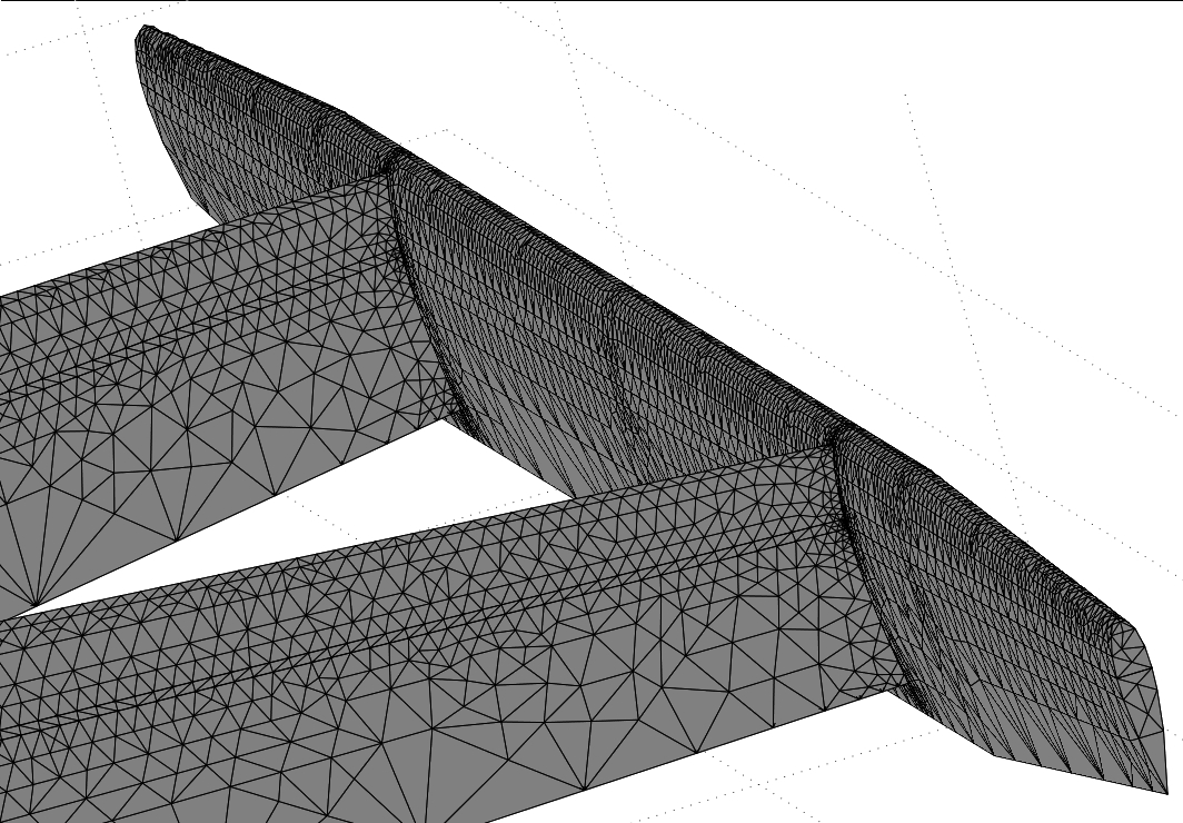
In the FEM programs used in this project [11][12] a geometry is drawn after which a mesh is

defined. The continuous domain is discretized into a set of discrete sub-domains (see figure 1.3).

Figure 1.3: A typical mesh on the surface of a 3D geometry.

Chapter 2

Designing of the turbine

2.1 Introduction

The turbine is the first part designed in this project. Besides the primary objectives (stated in the

objective function) no extra constraints are introduced due to properties of the other structural

parts (tower and generator).

2.1.1 The chosen wind turbine concept

The H-rotor concept

The turbine design presented here is a VAWT with straight blades supported with struts and

is named an H-rotor (see figure 2.2). This concept is developed at the Division for Electricity

and Lightning Research, Uppsala University. The H-rotor is omni-directional and needs no yaw

mechanism. Due to the straight blades, and constant speed along the blades, a simple blade profile

can be used. The axis orientation enables the generator to be placed on ground. By this a lighter

tower structure is needed. The shaft is directly connected to the generator which eliminates the

gearbox. An electrical controlled passive stall regulation is used without the need of pitching the

blades. Simplicity is the main advantage of this concept [13].

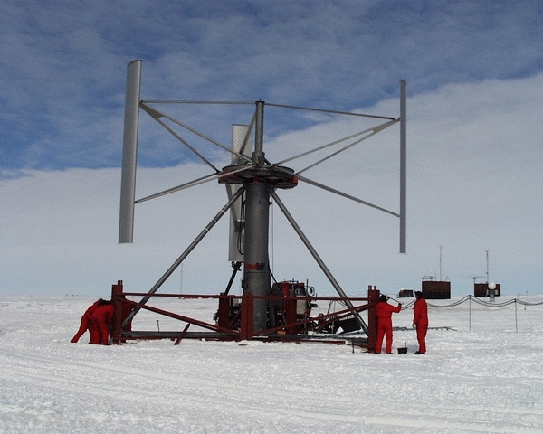
A similar design was installed in 1991 at the German Georg von Neumayer Antarctic station

(70

S; 8

W ). It is a three bladed H-rotor type vertical axis wind turbine named HMW-56

(see figure 2.1). The turbine has a diameter of 10 m and a total swept area of 56 m

. The rated

power is 20 kW in 9 m/s. The generator is mounted in the top of the tower with the turbine

struts directly connected to the outer rotor of the generator. The steel tower is able to be lifted

mechanically by a winch. HMW-56 is a prototype wind turbine especially designed for the harsh

climate in antarctica and it is still operating. The electric converter and control unit had to be

replaced after three years of operation, but no mechanical damages have occurred and very little

maintenance has been needed [14][5].

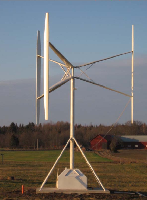
The H-rotor prototype project in Marsta

A 12 kW H-rotor has been installed in Marsta, outside of Uppsala Sweden, in December 2006 (see

figure 2.2). The turbine has a swept area of 30m

at 6m height. The generator is placed on ground.

The purpose of this installation is to perform various measurements in order to validate models

used in the design process and to prove the viability of the concept [13].

Figure 2.1: The HMW-56 wind turbine operating at the German Georg von Neumayer Antarctic station.

Figure 2.2: The 12 kW H-rotor placed in Marsta.

2.2 Design strategy

The following strategy is used in the design of the H-rotor turbine:

1. Gather meteorological data and describe the wind resource on site.

2. Define the objective function (state the most important design criteria).

3. List the parameters encountered in the design procedure. This is a mean of defining the level

of detail in the analysis.

4. Fix some parameters to simplify and shorten the amount of time needed for the design

process.

5. Based on the wind resource on site and performance data of earlier designs find a first

tentative design fulfilling the power demand.

6. Refine the tentative design using a design tool to ensure that all parts in the objective function

are achieved. To further simplify the design process it is performed assuming fixed turbine

radius and blade length (denoted the reference design). As the optimum rotor solidity is

found, scaling the reference design is made possible without loosing the overall aerodynamic

performance. One parameter at a time is optimized and then hold fixed in the following

order.

• Rotor solidity

• Blade profile thickness

• Fixed blade pitch

• Point of attachement

7. Choose a control strategy.

8. Based on comparisons between measurements on earlier designs and outputs from the simu-

lation tool introduce a reduction factor on the aerodynamic efficiency.

9. Scale the optimized reference design to meet the mean power demand stated in the objective

function.

10. Verify the mean power output using the known wind regime and simulated aerodynamic

performance. That produces a power curve. Calculate the yielded number of MWh produced

per year.

It was also remarked later in this work that another parameter can come into consideration; the

number of turbines. The first approach was to design one 5 kW turbine. However, due to an extra

constraint appearing later in this work, two turbines of 2.5 kW and five turbines of 1 kW are also

investigated. These special designs will be investigated in the paragraph 2.10 "Alternative number

of turbines, two 2.5 kW, five 1 kW".

2.3 Wind resources

2.3.1 Data resources

The meteorological data used has been kindly provided by the Antarctic Meteorological Research

Center (AMRC) [15] which archives and provides the U.S. Antarctic Programe (USAP) [16] with

meteorological data. One minute averages of wind speed, temperature and pressure have been

measured since February 2004. One minute averages represent the highest possible resolution

stored by AMRC. The measuring mast is situated in the prevailing wind direction upwind of the

station to minimize disturbances caused by man made structures. Based on these data, mean wind

speed, wind speed frequency distribution and mean air density can be investigated.

2.3.2 Treatment of data

To evaluate the wind resource and the wind power production potential on site the meteorological

data is treated with statistical methods. The method used separates the data into wind speed

intervals or bins in which it occurs. A series of N wind speed observations is assumed. The data

are separated into N

bins of width w

, with midpoints m

and with the number of occurrences

in each bin (the frequency) f

such that:

N =

j=1

(2.1)

With this technique the mean wind speed is calculated using equation 2.2.

U =1

j=1

(2.2)

The mean machine power output for each wind speed bin, P

), defined by the machine power

curve is given later in the design process. This is then used to calculate the mean power production

(see equation 2.3). Based on P

) the estimated energy production E

can be calculated

(see equation 2.4).

j=1

(2.3)

j=1

(2.4)

2.3.3 Mean wind speed

The mean wind speed at a height of 10 m, corresponding to the first estimation of the turbine hub,

is 5.8 m/s. The wind speed measurements are performed between February 2004 to May 2007.

2.3.4 Wind speed frequency distribution

Figure 2.3 shows the wind speed frequency distribution. Every bar in the diagram represents the

frequency of occurrence for that special wind speed interval. Wind speeds between four and five

meters per second are the most common and represent around 40 percent of the time. Wind speeds

above 15 meters per second are very rare. The highest wind speed ever measured on the South

Pole is 24.6 meters per second.

Wind speed (m/s)

Frequencyofoccurence(%)

Figure 2.3: Wind speed frequency distribution.

2.3.5 The design wind speed

The power in the wind is proportional to the cube of the wind speed according to equation 1.1.

To design a wind turbine that maximizes the power output, rather than operation hours, it is the

root cube mean value of the cubed wind speed that set the design criteria. The root mean cube

value of the wind and thus the wind speed used during the design process is 6.7 m/s.

2.3.6 Density of the air

The density of the air is proportional to pressure and temperature defined in the general gas law

(see equation 2.5). The mean density used in further analysis is 1:07kg=m

. The density is low at

the South Pole because of the high altitude, about 2800 m, and thereby the low air pressure.

p = ˆ

(2.5)

where p denotes the pressure, ˆ the density, R is the gas constant, M is the molar mass and T is

the temperature of the air.

2.4 Objective function

The objective functions are:

• The power output for the wind distribution at the South Pole (maximize but with constraint

that it should be on average more than 5 kW).

• The aerodynamic efficiency, C

ˆAU

(maximize)

• Limit the fatigue on all parts (the design must not have unfavorable load patterns during

operation)

• The cost of the system (minimize)

2.5 Design parameters

The parameters listed below can be varied in the design process.

• Number of blades

• Turbine radius (m)

• Blade length (m)

• Blade chord length (m)

• Blade profile type

• Fixed blade pitch angle (degrees)

• Attachment point of the struts on the blade (m)

• Design of struts (blade profile and chord length)

• Rotation speed as a function of the wind speed (rad/s, rpm)

With these parameters it is possible to form some non dimensional numbers, namely:

• The solidity of the turbine (

)

• The ratio between the blade tip speed and the wind speed, the tip speed ratio (TSR)

• The aspect ratio (chord to blade length ratio) (

)

• The chord to radius ratio (

)

where N denotes the number of blades, c the chord length, R the turbine radius and H the length

of the blades.

2.5.1 Fixed parameters

All the design parameters are not free. Some can be chosen freely by the designer, such as the

rotational speed as function of the wind speed (namely the maximum rotation speed allowed).

Other parameters are held fixed to shorten the amount of time needed. Following parameters are

held fixed:

• Number of blades: 3

• Optimum TSR: 4

• Blade profile type restricted to symmetrical airfoils

• Struts blade profile: NACA 0025

The choice of three blades is mainly motivated by the reduction in complexity. Unpublished results

of reference [17] show that favorable load variations on the turbine may be achieved with more

than three blades but a higher manufacturing cost. An optimum TSR of 4 is chosen as it is in the

range of earlier VAWT designs and has proved to be viable for the prototype turbine in Marsta.

Only symmetrical NACA profiles are examined in this analysis. This is motivated by the signif-

icantly reduced costs associated with production of symmetrical profiles compared to cambered

profiles. The higher production costs of cambered profiles is due to the necessity of constructing

two molds to produce the up- and downside of the blade profile. NACA 4 digit symmetric profiles

are derived from polynomial shapes which make them easier to construct. Moreover, if all possible

blade profiles were to be investigated this would become a very large project of its own.

Simulations with different designs of the struts are not performed as they have small influence on

the aerodynamic efficiency. More importantly, the structural constraints put limitations on the

choice of struts dimensions. A NACA 0025 airfoil section is considered a good trade off between

aerodynamic performance (low resistance) and structural strength.

2.6 Estimation of a tentative design

The optimization tool, described in section 2.7.1, does not find an optimal design automatically

because a global optimum may not exist. Therefore a first guess is needed to start optimizing

and save time. Some parameters of the Marsta H-rotor prototype are used to start up the design

procedure.

The Marsta H-rotor is a 12 kW turbine rated at 12 m/s which has been both simulated and

experimentally studied. All design parameters of this turbine can be found in reference [13]. The

optimal TSR (TSR at optimal C

for use in the variable speed range) has been set to four. The

maximum blade tip speed has been set to 40 m/s. Three blades are used in order to reduce the

structural load variations without affecting the overall performance. The struts are made from

NACA 0025 profiles to be able to withstand centrifugal loads and extreme aerodynamic loads.

Using the known wind speed frequency distribution on the South Pole and the experimental C

vs. TSR curve for the H-rotor in Marsta, enable calculations for a tentative design. The tentative

design procedure is to scale up the 12 kW H-rotor until the mean power output is around 5 kW.

This tentative design procedure suggests a rotor with approximately a radius of 5m and a blade

length of 10m. All other parameters listed in section 2.5 are held the same as for the H-rotor in

Marsta.

2.7 Optimizing the tentative design using a CMDMS model

The tentative design does not achieve all demands in the objective function. Therefore a fine tuning

is needed. To do this in an effective way a simulation tool is used. Throughout the design process

the results from the simulations are qualitatively compared with experimental data or results from

other models used in similar applications.

2.7.1 The CMDMS model

The model used during the design process is a CMDMS (Conformal Mapping and Double Multiple

Streamtube) model. The CMDMS model is based on the ideas of the Double Multiple Stream-

tube (DMS) model presented in reference [18]. All design parameters listed in section 2.5 can be

changed in the program. The CMDMS model uses a double step momentum model to simulate

the aerodynamics of the vertical axis turbine. The airflow is split into an overall and a local part.

The model of the local part of the flow uses conformal mapping to describe the blade profile as a

circle. This enables faster calculations using Fourier Transforms. Reference [13] gives an additional

description of the used CMDMS model.

This model provides the aerodynamic forces. The outputs primary studied in this analysis are :

• The aerodynamic efficiency, C

• The tangential force coefficient, C

, plotted versus the blade position around one revolution

• The normal force coefficient, C

, plotted versus the blade position around one revolution

• The lift force coefficient, C

, plotted versus the local angle of attack

• The drag force coefficient, C

, plotted versus the local angle of attack

The CMDMS code was applied to obtain a C

vs. TSR curve on the Marsta 12 kW turbine. From

initial measurements it was indicated that the CMDMS code overestimate the results by 20%. This

will be taken into account in the final design stage.

The CMDMS model needs some necessary inputs to simulate the aerodynamics of the turbine

properly. One important input is the specification of the pre stall lift point. At a certain angle of

attack (AOA) the blade starts to enter the stall region and the C

slope starts to decrease. This

is nearly where the C

versus angle of attack curve ceases to be linear. In figure 2.4 this region

is presented for a NACA 0012 profile at various Reynolds numbers (caused by varied TSR). From

this point, and for higher values of AOA, the CMDMS model uses interpolated C

’s between the

given input and flat plate lift values for high angles of attack.

This characteristic of the program makes the analysis very sensitive to the chosen value of the pre

stall point. Ideally this input should be given by experimental lift AOA curves.

0.5

1.5

AOA (degrees)

2.5

3.5

4.5

5.5

Figure 2.4: Pre stall- and stall region for a NACA 0012 at different TSR’s.

2.7.2 Problem finding input data

There is a lack of experimental data in the pre stall region for some symmetrical NACA profiles due

to the low Reynolds numbers considered. For NACA 0018 and NACA 0021 sufficient experimental

data has been found in order to extract useful inputs for the multiple stream tube model [19][20].

The data source has a major influence on the outcome of the simulation. The simulated values

of C

are very sensitive to the assumed variation of airfoil characteristics with varying Reynolds

number. A particular care in the choice of aerodynamic airfoil data is highly recommended.

To compare at least qualitatively different airfoil sections and turbine designs, it is better to use

one unique tool. This tool should be as low demanding in terms of CPU time as possible. Based

on this a program named XFoil is chosen.

Description of XFoil

XFoil is a code used to simulate the aerodynamic properties for different airfoil sections in arbitrary

Reynolds number [21]. The outputs from XFoil are the aerodynamic lift coefficients versus angle

of attack in the pre stall region. From these data, a point from where the CMDMS program

starts interpolating the C

versus angle of attack curve can be chosen. The data from XFoil

seems conservative compared to the experimental data found for the NACA 0018 and NACA 0021

profiles.

XFoil incorporates a two-dimensional panel code, with coupled boundary layer codes, for airfoil

analysis work [21]. The turbulence level of the incoming airflow can be varied. For this application

the highest possible turbulence level is chosen motivated by the disturbed flow regime in the

"backside" of the turbine.

2.8 Designing of one 5 kW turbine

2.8.1 The reference design

Beside the fixed parameters listed in section 2.5.1 the design procedure is simplified furthermore

by assuming a fixed dimension of the turbine in the beginning of the designing process. This size

of turbine is denoted in this report as the reference design. A comparative study between fewer

parameters is made possible. The reference turbine is given a radius of 5m and a blade length of

10m.

These dimensions are based on the tentative design procedure which approximately suggests a

turbine of this size (see section 2.6). Table 2.1 summarize the parameters of the reference design.

Number of blades

Optimum TSR

Radius (m)

Blade length (m)

Blade chord length (m)

will be optimized

Airfoil section

will be optimized

Fixed pitch angle (deg)

will be optimized

Point of attachment

will be optimized

Struts design

NACA 0025 with same chord length as optimized blade design

Table 2.1: Parameters of the reference design.

The reference design is tested for variations in solidity, blade profile thickness, fixed blade pitch

and point of attachment in mentioned order. When choosing the turbine with best performance,

not only C

at the optimal TSR concludes what design that performs the best. In most of the

design steps, the lift- and drag coefficients as well as the tangential and normal forces transferred

to the struts are studied to avoid unfavorable characteristics. This is done with respect to the

objective functions specified in section 2.4.

When the best performing reference design is chosen it will be scaled down (with respect to the

swept area) to more exactly meet the mean power output demand. The last step is to redo

the design process in a simplified way to ensure that the scaling process did not deteriorate the

aerodynamic performance.

2.8.2 Optimizing the solidity

In the analysis of the optimum solidity the chord length for two different blade profiles is varied.

The rest of the parameters in the reference design are held fixed. The TSR is fixed and equals

four.

Influence of the solidity

Experiments compared with a very simple stream tube model has been performed by reference [22]

on a 12 ft. diameter darreius shaped vertical axis wind turbine. Results between both wind tunnel

experiments and simulations in these experiments correspond reasonably. The results suggest that

lower solidity generates a wider operating range in means of TSR’s.

A higher solidity generally makes the structure endure higher stresses and achieve maximum aero-

dynamic efficiency at lower TSR’s.

Numerical results from a DMSV model

Numerical experiments have been performed by reference [23] and [17] developing and using a

DMSV (Double Multiple Streamtube Variable) model. The DMSV model is based on ideas of

the DMS model presented in reference [18]. The major difference is that the DMSV model apply

variable flow reduction factors in both altitude and latitude direction between the two actuator

discs. Figure 2.5 present the C

vs. TSR curve for an H-rotor in the same range of Reynolds

number.

1234567

−0.05

0.05

0.1

0.15

0.2

0.25

0.3

3 blades chord=0.2m

= 0.15

3 blades chord=0.3m

= 0.225

3 blades chord=0.4m

= 0.3

3 blades chord=0.5m

= 0.375

Figure 2.5: C

vs. TSR curve for the an H-rotor turbine in the same range of Reynolds number.

Numerical simulations using the CMDMS model

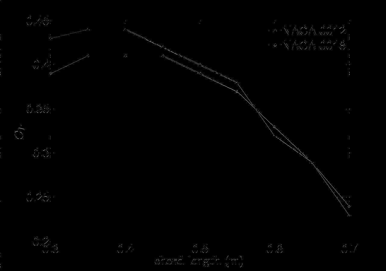
Based on simulations performed by reference [22] and [23] a first guess for an optimum rotor solidity

is 0.3 to achieve an optimum C

at TSR four. A rotor solidity of 0.3 with a design using three

blades and a radius of 5m results in a blade chord of 0.5m. To verify this assumption, simulations

in the CMDMS model have been performed. This has been done for two different symmetrical

blade profiles, NACA0012 and NACA0018. The solidity has been varied between 0.18 and 0.42

implying a chord length from 0.3m to 0.7m. The results from these simulations are presented in

figure 2.6.

Design chosen

Based on the results using the CMDMS model a solidity of 0.27 is chosen, which implies a blade

chord of 0.45m. This solidity is found near the maximum in both the DMSV and CMDMS model

and can meet the demand of a strong structure. The C

P max

is different between the turbines

modeled for using the DMSV and the CMDMS code respectively. This is because the turbines

used in respectively simulation are of different size and hence have various performance. None the

less it is possible to compare the aerodynamic performance qualitatively for varying TSR’s.

Figure 2.6: Aerodynamic efficiency with varying rotor solidity.

2.8.3 Optimizing the blade profile thickness

In the analysis of the optimum blade profile thickness the blade thickness is varied from 12 to 25

percent of the chord length. The TSR is varied for every blade profile between 2 and 6. The blade

chord length is set to 0.45m. The rest of the parameters in the reference design are held fixed.

Influence of the blade thickness

Numerical experiments presented in reference [24] suggest that neither C

P max

, nor the optimum

TSR, are significantly affected by the type of airfoil used on a VAWT with two skipping-rope shaped

blades. However, the blade stall characteristics and the aerodynamic efficiency are different. For

instance, a NACA 0012 blade profile generally achieves a slightly higher C

P max

and has higher

aerodynamic performance in higher TSR, while both NACA 0015 and NACA 0018 perform better

in the low TSR region. This is because thicker NACA profiles have better stall characteristics at

low TSR where the angle of attack varies in a larger span. Structural strength motivates a choice

of a thicker blade profile.

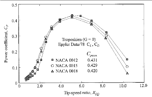
Numerical results from a DMS model

In figure 2.7 the C

is compared between three symmetrical airfoil sections at different TSR. In

this particular case the aerodynamic performance is simulated in a DMS model for a two bladed

rotor with skipping-rope (ideal Troposkien) shaped blades [24].

Numerical simulations using the CMDMS model

To verify that C

P max

occurs at tip speed ratio four for each blade profile, as earlier simulations

suggest [24], several simulations with the CMDMS model have been performed. Results from these

simulations are presented in figure 2.8.

Discussion

The results for the NACA 0012 blade profile does not correspond well with the experiments per-

formed by reference [24] in this analysis using the CMDMS model. The NACA 0012 blade profile

Figure 2.7: C

vs. TSR for three different NACA profiles simulated with a MDS model [24]. X

denotes

the TSR on the equatorial section of the curved blades.

performs well at low TSR and has a lower optimum TSR. This is probably an artifact in the code

due to the unstable numeric caused by thin profiles at high angles.

Moreover, it is to remember that the numerical simulations performed using the CMDMS model

and the DMS model (as in reference [24]) differ in number of blades and turbine blade geometry. A

straight bladed H-rotor have the same Reynolds number and AOA along the whole blade whilst a

turbine using skipping-rope shaped blade does not. These aspects explain the differences between

the two simulations.

Chosen design

The results using the CMDMS model reveal that a NACA 0018 blade profile seems to be a well

suited trade off between aerodynamic performance and structural strength. Therefore the sym-

metrical NACA 0018 blade profile is chosen for the reference design.

2.8.4 Optimizing the fixed blade pitch

In the analysis of the optimum fixed blade pitch the offset angle is varied from 0 to +4 degrees.

Positive pitch angles are defined as toe out. Early tests showed that all negative fixed pitch angles

generated very bad results along with unfavorable load cycles. The TSR is varied for every blade

profile between two and six. The blade chord length is set to 0.45m and the blade profile is set to

NACA 0018. The rest of the parameters in the reference design are held fixed.

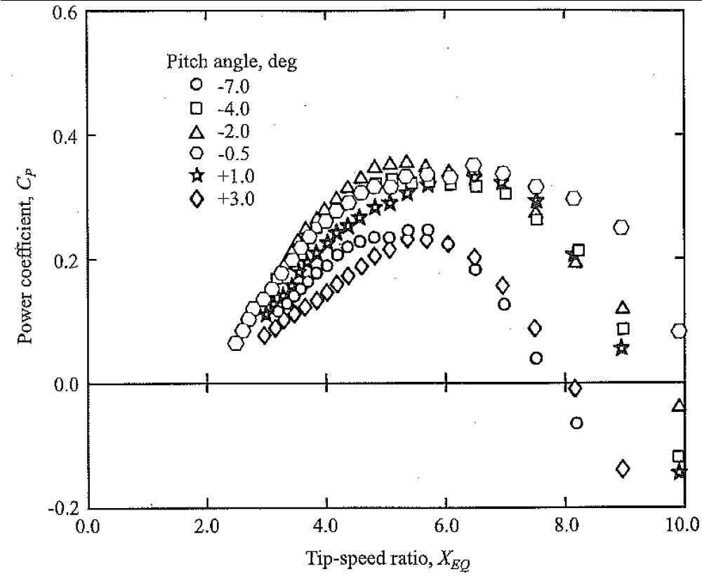
Influence of the pitch angle

Sandia National Laboratories have done tests on a 5m radius research turbine concerning the effects

of fixed blade pitch [25]. Significant variations in cut-in TSR, aerodynamic efficiency and maximum

power output have been shown. Changes as small as only one or two degrees can generate large

differences in result [26]. Reference [26] concluded that the aerodynamic performance is changed

when using a fixed blade pitch due to following reasons:

• The variation pattern in angle of attack is changed resulting in an altered blade torque

pattern around one revolution.

23456

0.05

0.1

0.15

0.2

0.25

0.3

0.35

0.4

0.45

0.5

NACA 0012

NACA 0015

NACA 0018

NACA 0021

NACA 0025

Figure 2.8: C

vs. TSR for five different NACA profiles.

• The normal force of the blade is able to contribute to the torque due to the offset between

the mounting position (angle) and the centre of pressure.

Experimental results from the Sandia 5m radius turbine

Performance data for the Sandia 5m radius research turbine suggests that variation in fixed pitch

angle is a powerful and simple tool for the designer to improve the turbine performance. Figure

2.9 shows performance data for the Sandia 5m radius research turbine. In these plots the pitch is

denoted positive for toe-in angles.

Figure 2.9: Experimental results on the Sandia 5m radius reserach turbine. X

denotes the TSR on the

equatorial section of the curved blades.

Numerical simulations using the CMDMS model

The impact of pitching the blades has been investigated by doing several simulations with the

CMDMS model. Results from simulations using a NACA 0018 airfoil are shown in figure 2.10.

23456

0.05

0.1

0.15

0.2

0.25

0.3

0.35

0.4

0.45

0.5

0 deg

+1 deg

+2 deg

+3 deg

+4 deg

Figure 2.10: C

vs. TSR for a NACA 0018 blade profile with chord 0.45m for varying fixed pitch angle.

Discussion

A pitched blade achieves a much higher aerodynamic efficiency, especially around the region of

optimal TSR. The major explanation for this seems to be the possibility to move the region of

blade stall around the blade revolution.

Chosen design

Based on these results a constant pitch of +4 degrees looks promising for the reference design.

From an operation point of view it is preferable to have a wide and smooth C

vs. TSR curve in

the region around the optimal tip speed ratio.

2.8.5 Optimizing the point of attachment

In the analysis of the optimum point of attachment the mentioned parameter is varied between 0

to 50 percent of the chord from the leading edge. The TSR is held fixed at four. The blade chord

length is set to 0.45m, the blade profile corresponds to NACA 0018 and a fixed blade pitch of four

degrees is used. The rest of the parameters in the reference design are held fixed.

Influence of the attachment point

The point of attachment is where the struts are mounted on to the blades and is denoted by

percent of the chord from the leading edge. Unpublished results based on numerical simulations

by reference [17] suggests variations in both aerodynamic performance and load patterns on the

turbine when changing the point of attachment (see figure 2.11).

(a) The normal force coefficient plotted for one revolution.

(b) The tangential force coefficient plotted for one revolution.

Figure 2.11: Influence of the attachment point. LE denotes the leading edge.

Numerical simulations using the CMDMS model

The effects of change in the point of attachment were simulated at 10, 20, 25, 30, 40 and 50 percent

of the chord length. As can be seen in figure 2.12, the effect on the aerodynamic performance of

changing the point of attachment is very small using the CMDMS model. The tangential and

normal forces transferred to the struts from the blades showed very little difference between the

different attachment points.

0.1

0.2

0.3

0.4

0.5

0.454

0.456

0.458

0.46

0.462

0.464

0.466

Figure 2.12: C

with varying point of attachment for the fully optimized 2.5 kW design.

Discussion

The very small effects on the performance when varying the point of attachment may be due to

the code used (CMDMS) not capable of properly simulating the influence variations in attachment

points.

Chosen design

Based on these results using the CMDMS model the point of attachment is chosen to be at 25

percent of the chord from the leading edge, also denoted the "quarter chord". This is the normal

configuration in most designs and because of the very small difference in C

there is no motivation

why to change this.

2.8.6 Control strategy

The control strategy is a way of defining the rotation speed as a function of the wind speed. For this

application the control mechanism is based on passive stall regulation governed by the generator.

The shape of the power curve will depend on the optimal tip speed ratio and the maximum blade

tip speed allowed. The turbine is designed to operate at TSR four. As soon as the blade tip speed

reaches 40 m/s the rotational speed will be fixed to limit the centrifugal forces acting on the blades

and the struts (see figure 2.13). As can be seen in figure 2.14(a), the turbine benefit from the stall

regulation after the rotational speed has been fixed and the power output is reduced. At wind

speeds above 20 m/s a controlled shut down will be administrated not shown in the figure 2.14(a).

2.9 The proposed 5 kW design

The above optimized reference design resulted in a mean power output of 5.2 kW after a 20 percent

reduction of the theoretical C

(every C

point along the C

vs. TSR curve). Therefore, scaling

Windspeed (m/s)

Rotationalspeed(rpm)

Figure 2.13: Control strategy in means of revolutions per minute versus the wind speed for the fully

optimized 5 kW turbine.

of the optimized reference design is not needed to meet the mean power demand of 5 kW in the

objective function.

The mean power output is calculated using equation 2.3 incorporating the real wind speed frequency

distribution and the control strategy described above. Moreover, the theoretical C

P max

value is

decreased with 20 percent to a more realistic value around 0.38 at optimum TSR.

Table 2.2 summarize the design parameters for the fully optimized 5 kW wind turbine. Figure

2.14(a) and 2.14(b) present the power curve and C

vs. TSR curve respectively.

Mean power output (kW)

5.2

Number of blades

Radius (m)

Blade length (m)

Blade chord length (m)

0.45

Airfoil section

NACA 0018

Fixed pitch angle (deg)

Point of attachment

0.25 times the chord length

Struts design

NACA 0025 with chord length 0.45

at TSR four

0.38

Table 2.2: Optimized parameters for the 5 kW wind turbine.

2.10 Alternative number of turbines, two 2.5 kW, five 1 kW

Initially, the objective was to design one wind power machine producing 5 kW mean power output.

The smallest turbine meeting this demand turned out to have a radius of 5m and blade height of

10m (see section 2.9). As this size of turbine may not be suitable for this special application, a

strategy of designing several smaller wind turbines emerged. Two turbines, one with 1 kW and

another with 2.5 kW mean power are proposed.

When scaling down a design, both aspect ratios and the solidity have to be kept constant. This

is due to preserve the aerodynamic behavior of the turbine. As can be seen in figure 2.15, the

aerodynamic behavior seems to be kept constant within an acceptable range.

Table 2.3 contains the two turbine designs which evolved when scaling down for 2.5 kW and 1.0

kW respectively. Figure 2.16 summarize the performance for both of the designs. The mean power

output is calculated using equation 2.3 incorporating the real wind speed frequency distribution

and the control strategy described in section 2.8.6. Moreover, the theoretical C

value is decreased

with 20 percent to a more realistic value at the optimum tip speed ratio for both of the designs.

The 12 kW rated power turbine in Marsta turned out to have a mean power output of about

1.3 kW in this wind regime. Therefore this design is chosen for the 1.0 kW application. Though

the Marsta design has slightly different aspect ratios and solidity, the aerodynamic performance is

estimated to be sufficient. The 12 kW rated power design in Marsta is favored as it represents an

effective choice compared to the reconstruction of a new design.

Mean power output (kW)

2.8

1.4

Number of blades

Radius (m)

3.75

Blade length (m)

7.5

Blade chord length (m)

0.35

0.25

Airfoil section

NACA 0018

NACA 0021

Fixed pitch angle (deg)

Point of attachment

quarter chord

Struts design

NACA 0025, chord=0.35m NACA 0025, chord=0.25m

at TSR four

0.37

0.32

Table 2.3: Optimized parameters for the 2.5 kW and 1 kW wind turbines.

The real mean power output of the 2.5 kW design is 2.8 kW with a 20 percent reduction of the

theoretical C

. The mean power output calculations are based on the real wind speed frequency

distribution. The maximum C

is 0.37 at TSR four.

The real mean power output of The 1 kW design is 1.4 kW with a 20 percent reduction of the

theoretical C

. The mean power output calculations are based on the real wind speed frequency

distribution. The maximum C

is 0.32 at TSR four.

Wind speed (m/s)

Power(kW)

(a) Power curve for the 5 kW turbine.

12345678

−0.05

0.05

0.1

0.15

0.2

0.25

0.3

0.35

0.4

TSR

(b) C

vs. TSR curve for the 5 kW turbine.

Figure 2.14: Power curve and C

vs. TSR curve for the 5 kW turbine. Optimum TSR is four. The

controlled shut down of the turbine at 20 m/s is not shown in the figures.

23456

0.05

0.1

0.15

0.2

0.25

0.3

0.35

0.4

0.45

0.5

TSR

Optimized reference design

2.5kW design

Figure 2.15: C

vs. TSR for the fully optimized reference design and the 2.5 kW turbine after preservation

of the rotor solidity and aspect ratios.

Wind speed (m/s)

Power(kW)

(a) Power curve for the 2.5 kW turbine.

Wind speed (m/s)

Power(kW)

(b) Power curve for the 1 kW turbine.

1234567

−0.05

0.05

0.1

0.15

0.2

0.25

0.3

0.35

0.4

TSR

vs. TSR curve for the 2.5 kW turbine.

1234567

−0.1

−0.05

0.05

0.1

0.15

0.2

0.25

0.3

0.35

TSR

(d) C

vs. TSR curve for the 1 kW turbine.

Figure 2.16: Power curve and C

vs. TSR curve for the two smaller wind turbines. Optimum TSR is four

in both designs. The controlled shut down of the turbines at 20 m/s is not shown in the figures.

Chapter 3

Load estimates and stability

calculations on the foundation

3.1 Introduction

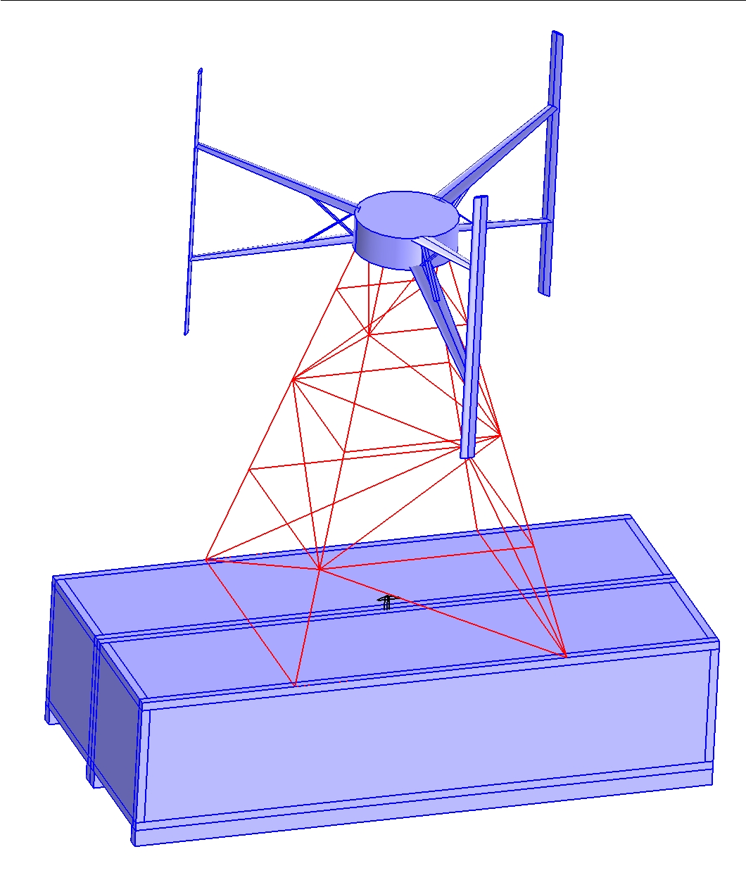
The foundation in this application consists of two eight feet (2.4 m) wide by 34 feet (10.4 m) long

containers bolted into a foundation as can be seen in figure 3.1. Both containers are eight feet

(2.4 m) high and their total weight together is about 13600 kg. Two skis, one foot (0.3 m) wide

by 34 feet (10.4 m) long, are mounted on the bottom of each container to enable movement of the

structure. The main reason for mounting the wind turbine on top of the containers is that these

are controlled by the ICECUBE project. This means that they can be modified with minimal

permission from Raytheon Polar Services Corporation (RPSC) or National Science Foundation

(NSF). A permanent mounted structure will need more approvals [27].

Verifying whether the proposed double mounted container structure will work as a foundation

does not include any designing. First the loads are estimated then calculations and simulations

are performed to verify the constraints stated on the foundation. The stability of the foundation

is tested before optimization of both the tower and generator. It is important that the designed

turbine is not too large. Once the tower and the generator are optimized the stability calculations

on the foundation is performed again. This time with more accurate input data.

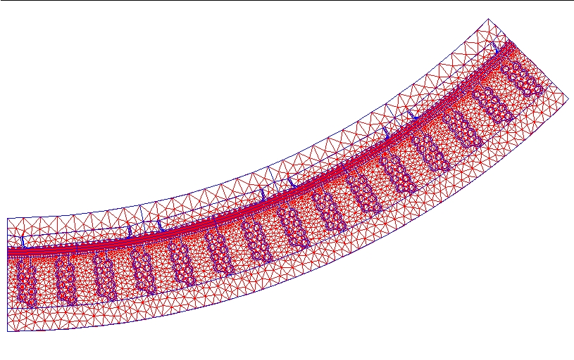
3.2 Simulation tool used in the structural mechanic analysis

The simulation tool used when analyzing stress and strain cases as well as the eigenfrequency of

both the foundation and the tower structure is COMSOL Multiphysics 3.3 (formerly FEMLAB)[11].

COMSOL is a solver software package for various physics and engineering applications using Finite

Element Methods. Using a FEM program like COMSOL is time saving for this project as the

geometries, in for example the foundation and tower structure, are complex. Still, the geometries

have to be simplified before running a simulation in COMSOL to reduce CPU time. This is

achieved by modeling the structure with shells and beams. Solids should be avoided as the number

of equations solved for is directly proportional to the degrees of freedom.

3.3 Load estimates

There will be mainly three load cases present. Static loads due to the weight. Static pressure

loads due to the wind. Unsteady loads due to flow induced vibrations and unsteady thrust forces

for the turbine. The loads and assumed geometries in the calculations are in most cases slightly

exaggerated to generate results on the safe side. The load estimates presented in this section will

also be used in the design of the tower structure.

3.3.1 Weight loads

The static load transferred to the underlying snow includes the weight of the foundation, tower,

turbine and generator. The weight of these components acts as a vertical pressure force on the

snow under the four skis. The approximated weights of the different components are summarized

in table 3.1. The turbine weights are based on the actual weight of the H-rotor in Marsta. The

turbine weight estimates are calculated with a scaling law using the cubic relationship between

the masses and lengths. The tower weights are based on the chosen designs presented in table 4.1.

The generator weights are based on the chosen designs presented in table 5.2.

Turbine design

5 kW 2.5 kW 1 kW

Foundation (kN)

133 133 133

Truss tower (kN)

Turbine (kN)

2.5

0.5

Generator (kN)

2.5

Total static load, W (kN) 179.5 183 189

Table 3.1: Approximated weights of the different components. The truss towers are lighter for the larger

turbines due to lower constraints on the eigenfrequency.

3.3.2 Static pressure forces and torques due to the wind

The static pressure load is the load caused by the wind acting on the entire structure. In equation

3.1 A denotes the projected frontal area facing the wind.

P ressure

ˆv

air

(3.1)

Drag

= F

P ressure

(3.2)

, denoting the drag coefficient in equation 3.2, depends on the shape of object exerted by the

wind. For the container foundation and the generator house a drag coefficient of 2 is used, the

same as for a long flat plate perpendicular to the air flow. For the cylinder shaped truss members

in the tower a drag coefficient of 1.3 is used. The static pressure loads on the turbine is simulated

using the CMDMS model described in section 2.7.1.

Torque is caused by drag force, defined in equation 3.2, acting on the structure surface facing the

wind.

Estimating the load torque caused by the wind hitting the foundation, tower and

generator house

Drag

is approximated for a maximum wind speed of 40 m/s during stand still of the turbine.

The wind hitting the structure will cause a load torque. The area of the different structural parts

facing the wind is estimated and presented in table 3.2.

Turbine design

5 kW 2.5 kW 1 kW

generatorhouse

) 1

tower

)

7.5

foundation

)

Table 3.2: Estimated areas for calculation of the static pressure load torque.

The area estimates assume that the wind is hitting the wind turbine structure perpendicular to

the long side of the containers to achieve the maximum load torque possible. These estimates

assume that the same tower construction and generator house dimensions are used for all three

turbine designs. Area estimation of the tower is using the dimensions presented in section 4.8.

The area of the truss tower is estimated assuming a solidity of 20% ((truss member projected

area)/(total enclosed area ot the truss tower)) whereafter a representative geometrical shape (an

uppright triangular) of the tower is used in further calculations.

The static pressure load torque caused by the wind hitting one area element of the structure, dM,

is calculated by multiplying the drag force per surface with the projected area element, dxdz,

and the height from the snow level, z. The total load torque caused by a structural part is then

calculated by integrating dM over the whole structure surface area S as described in equation 3.4.

Figure 3.1: The axes of orientation.

dM = dF

Drag

z =

ˆv

air

zdxdz

(3.3)

StructuralP art

(3.4)

This is done for the foundation, truss tower and generator house respectively and is presented in

table 3.3.

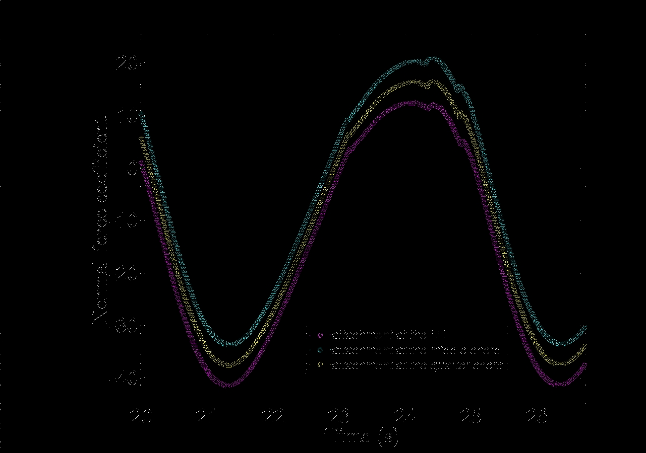
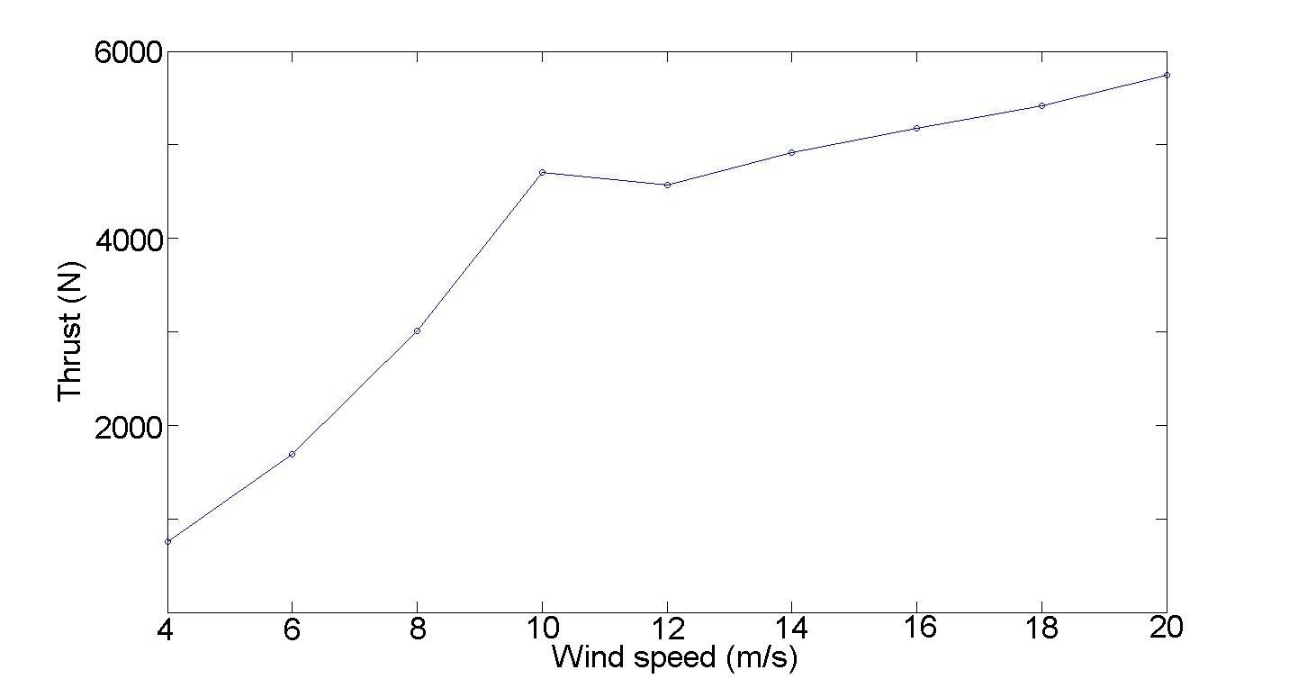
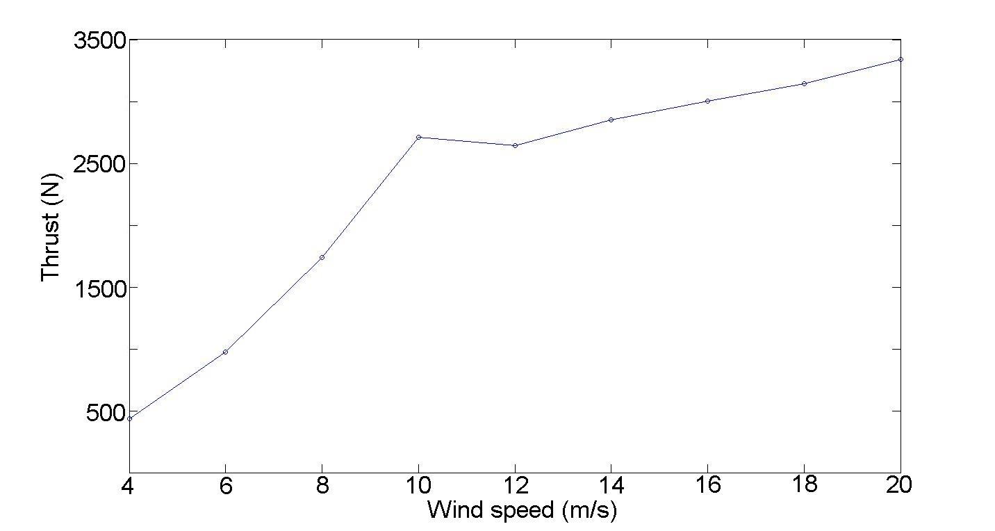
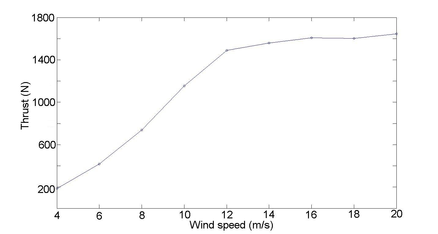
Simulation of the drag force on the turbine

Simulations on the three different turbines are performed for a wind speed of 40 m/s and a tip

speed ratio equal to zero (stand still). The results from one of these simulations are presented in

figure 3.2. The static pressure forces on the turbine is transfered to the hub. Therefore the static

pressure load torque contribution from the turbine is calculated by multiplying the simulated forces

with the height of the hub above snow level (10 m).

Figure 3.2: Forces transferred to the hub for the 5 kW turbine in 40 m/s during stand still. The straight

line is the mean value of the static pressure force on the whole turbine structure.

Total static pressure load torque

Table 3.3 present the sum of the static pressure load torque.

Turbine design

5 kW 2.5 kW 1 kW

turbine

(kNm)

107

generatorhouse

(kNm)

tower

(kNm)

foundation

(kNm)

Total pressure load torque, M

tipping

(kNm) 242 199 165

Table 3.3: Estimated load torque caused by the wind at 40 m/s during stand still.

3.3.3 Unsteady loads

Flow induced vibrations

Even at high Reynolds numbers a no-slip condition will hold for a fluid flowing next to a surface.

The no-slip condition imply that the fluid has zero velocity in the boundary between the surface

and the fluid. But it is confined to a small region, the boundary layer along the surface. For

streamlined bodies the flow outside the boundary layer is largely irrotational. For bodies with high

curvature (e.g. a cylinder) an adverse pressure gradient result in a region of backward flow and

deattached boundary layer. The region of circulation caused by the separation becomes unstable

at sufficiently high Reynolds numbers which will cause an oscillating wake. The wake is composed

of large scale eddies downstream of the body. The formation of these large scale eddies occur at a

dominating frequency f which is described in the non-dimensional form by the Strouhal number

(see equation 3.5) [28].

St =

(3.5)

In equation 3.5 St is the Strouhal number depending on the body geometry, 0.2 for a circle. L is the

characteristic length, for this application the diameter of the steel tubes used as truss members in

the tower. U is the free stream wind velocity. The periodically varying pressure forces on the body

caused by the vortex shedding may result in flow induced vibrations. This frequency is calculated

for a wind speed of four meters per second. Four meters per second is the assumed wind speed for

start up of the wind turbines. The results are presented in table 3.4.

Turbine design

5 kW 2.5 kW 1 kW

Flow induced frequency (Hz) 13

Table 3.4: Calculated flow induced frequencies at a wind speed of four meters per second.

Unsteady thrust on the turbine

Unsteady thrust forces on the turbine during operation result in time varying stresses in the

structure that may lead to fatigue damage. In figure 3.3 the thrust force on the 5 kW turbine is

plotted for one revolution. Each blade contribute with a highly varying thrust force (around one

revolution) as a function of the position. The sum of all three blades result in a somewhat sinus

shaped thrust force function.

−100

−50

100

150

200

250

300

−1000

1000

2000

3000

4000

5000

6000

7000

8000

9000

Thrust force on 5 kW mean power turbine at 20 m/s

One revolution (degrees)

Thrust force (N)

mean

thrust

resultant

thrust

force

thrust

contribution

from one

blade

Figure 3.3: Thrust forces transferred to the hub for the 5 kW turbine at 20 m/s.

Harmonics

As in many rotating mechanical systems not only the operational frequency (denoted P) is present.

Several overtones, harmonics, may occur. These overtones all have an integer multiple frequency

(nP) compared to operational frequency. In HAWT applications the most common type of har-

monic is the blade passing frequency. When a blade pass the tower shadow (in means of wind

speed) a change in thrust force and moment is induced. This result in a blade passing frequency

equal to the number of blades times the operational frequency. For VAWT applications a 3P fre-

quency is present due to the variation pattern of the tangential force for the three blades. A 6P

harmonic is also produced as each blade is passing the wakes of the other two blades per revolution.

Figure 3.4 present the different harmonics at different wind speeds for the 5 kW turbine.

Figure 3.4: Thrust force induced harmonics for the 5 kW turbine. ModC/mean(signal) present the total

variation in force as percentage of the mean thrust force for the actual wind speed.

To avoid resonance it is importat that none of the frequencies interfere with the eigenfrequency

of any structural part in the design. Resonance may lead to large deformations and associated

high loads. The operational frequency for different wind speeds will follow the control strategy

described in section 2.8.6. A Campbell diagram is drawn for each turbine (see figure 3.5) presenting

the operational frequency along with the 3P and 6P harmonics and the eigenfrequencies for the

foundation and tower (based on simulation 1 and 2 respectively).

3.4 Constraints and calculations

3.4.1 Overturning

To prevent the wind turbine structure from overturn the stabilizing torque generated by the weight

load has to be larger than the static pressure load torque. The weight load torque is calculated with

equation 3.6 where W denotes the weight and L denotes the foundation width. The foundation

width is approximated to 4.9m.

stabilizing

= W

(3.6)

Table 3.5 presents the dynamic and static load torques along with safety factors for each turbine

design.

Turbine design

5 kW 2.5 kW 1 kW

stabilizing

(kNm)

440 448 463

tipping

(kNm)

242 199 165

Safetyfactor K

overturn

at 40 m/s 1.8

2.2

2.8

Safetyfactor K

overturn

at 25 m/s 4.5

5.6

7.0

Table 3.5: Stabilizing and tipping moments acting on the wind turbine structure.

Wind speed (m/s)

Frequency (Hz)

Tower

Foundation

(a) Campbell diagram for the 5 kW turbine.

Wind speed (m/s)

Frequency (Hz)

Foundation

Tower

(b) Campbell diagram for the 2.5 kW turbine.

Wind speed (m/s)

Frequency (Hz)

Tower

Foundation

Figure 3.5: Campbell diagram for all three turbines. 4 m/s is the assumed start up wind speed, at 10 m/s

the rotational speed of the turbine is fixed.

When designing foundations the safety factor for overturn should be at least three. None of the

designs in table 3.5 can meet these standards during hurricane conditions (40 m/s).

3.4.2 Container strength

Installation of a wind turbine on top of the double container foundation will not result in exceeding

the static design load according to reference [29]. These containers are designed to withstand a

stacking pressure corresponding to eight fully loaded containers (950 kN). It is the frame of the

container that ensure the strength, the design loads of the roof is merely 3 kN [30].

3.4.3 Snow collapse and settlement

The foundation should be designed to minimize the effects of settlement caused by the wind turbine

operation and static weight.

No theoretical guidance could be found in the literature concerning the impact on the underlying

snow layers when exposed to a vertical pressure force. The weight added by the wind turbine,

generator and truss tower will be in the range of 10-15% (see table 3.1).

According to table 3.3.

3.4.4 Drift of the structure

Horizontal movement of the container foundation caused by forces on the structure during operation

or hurricane conditions is not allowed. This might be a problem because of the skis mounted

beneath the containers used for simplifying movement twice per year. Calculations are performed

only for the structure with the 5 kW turbine design as this concept will result in the highest

horizontal forces.

The coefficient of friction between the snow and the skis is about 0.1 [27]. By this, the maximum

horizontal force allowed transferred to the skis is 0:1 ? 179:5kN ˇ 18kN. The horizontal force at

stand still during hurricane conditions is described by equation 3.7. The horizontal force during

operation is described by equation 3.8. F

Dragturbine

and F

T hrustturbine

are simulated using the

CMDMS model. The drag forces on the structure include forces on the container foundation,

tower and generator house. Drag forces are estimated using the techniques described in section

3.3.2. The results are presented in table 3.6.

HorizontalHurricane

= F

DragStructure

+ F

DragT urbine

(3.7)

HorizontalOperation

= F

DragStructure

+ F

T hrustT urbine

(3.8)

As the skis are mounted along the long side of the containers all drag forces are calculated assuming

that the wind is hitting the short side of the containers.

Turbine design

5 kW

Horizontal

during operation (kN)

13.7

Horizontal

at hurricane conditions (kN) 42.2

Table 3.6: Horizontal forces transferred to the skis. The maximum horizontal force allowed transferred to

the skis is 18kN

3.4.5 Eigenfrequency

The eigenfrequency of the foundation must not coincide with the rest of the structure to prevent

effects caused by resonance.

The upper snow layer and the foundation is tested for eigenfrequencies in COMSOL. The model

used is of the entire tower structure and the foundation standing on top of a solid describing the

layers of snow.

The truss tower is given the properties presented in section 4.8. The foundation model is made of

shells given the right thickness and densities to give realistic vibration characteristics and weight.

The four skis are included in the foundation model. The upper snow layer is reproduced by

four layers of cylindrical solids. These are also given realistic values of density and vibration

characteristics. The density in the different snow layers are varied linearly from 380kg=m

in the

upper most layer to 540kg=m

in the lowest [31][32]. The elastic modulus is varied in the same

way from 170MP a to 1050MP a. The Poisson’s ratio is set to 0.2 in all layers [33]. The boundaries

at bottom and sides of the snow solid are held fixed in all directions.

Simulation 1: Eigenfrequency of the structure including upper snow layer and foun-

dation. The lowest eigenfrequency in this model is 7.0 Hz. This is true for all tower designs.

3.5 Discussion

3.5.1 Overturning

None of the turbine designs resulted in a safety factor above three at hurricane conditions. However,

all three turbine designs are estimated to be viable. This is motivated due to the highest wind speed

ever measured at the South Pole was about 25 m/s. At this wind speed the tipping moment would

decrease with 60% which leads to a higher safety factor as can be seen in table 3.5. Constructing

a support structure mounted on the long sides of the countainers would increase the stability. One

example of such a construction is sketched in figure 3.6(a).

Another method to prevent tipping of the structure is to use snow anchors. These would be buried

under a snow mass. The other end would be attached in the foundation structure as shown in

figure 3.6(b).

(a) Support arms.

(b) Snow anchors.

Figure 3.6: Sketched support structures. View from the short end of the container foundation.

A final option is to use a lower tower for the larger turbines to decrease the tipping moment.

3.5.2 Container strength

The container can easily withstand the static weight of the tower, generator and turbine. This is

true for a design where the weight is transferred to the frame of the container. The easiest way

to do this is to design a tower with a bottom width equal to the width of the double container

foundation.

3.5.3 Drift of the container foundation

It is a clear risk of drift of the container foundations at high wind speeds. The calculations are

most conservative as the coefficient of friction can be up to three times larger to start moving the

container [27]. In addition, a wind speed of 40 m/s is most unlikely. The highest wind speed ever

measured on site is about 25 m/s at which the horizontal force transferred to the skis are lower

than the maximum allowed (assumed stand still of the turbine). None the less, some type of wedge

construction mounted at the ends of the skis is suggested to avoid any risk of drift of the container.

3.5.4 Snow collapse and settlement

No extra settlement is to be expected due to the extra static weight when mounting a wind turbine

on top of the container. Whether the vibrations present during operation of the wind turbine

will result in settlements is hard to say. If it turns out that settlements occur due to vibrations,

installation of some extra pontoons to decrease the local pressure force could be one solution.

Change of skis to a wider type may also be a solution.

3.5.5 Eigenfrequency

The eigenfrequency of 7.0 Hz may result in vibration problems due to resonance phenomena. 7 Hz is

in the operation range for all three turbine designs though only for 3P and 6P operation frequencies

(see figure 3.5). The margin of error in simulation 1 is relatively large due to the uncertainty of

the elastic and vibration properties for the snow. The elastic and vibration properties used in

simulation 1 are for unpacked snow. In reality the snow is packed before placing the containers.

This may lead to stiffer snow characteristics and thereby a higher eigenfrequency for the whole

structure. Further analysis, preferable with a more accurate vertical density profile of packed snow,

is therefore highly recommended.

Chapter 4

Designing of the tower structure

4.1 Introduction

The main purpose of the tower structure is to elevate the turbine to the design height. Moreover,

the tower structure has to be stable and stiff enough to not interfere with the operation of the

wind turbine. As will be further explained in the generator section of this report, the generator is

suggested to be mounted in the top of the tower. By this, the tower structure has to withstand

the extra weight added compared to the earlier H-rotor structure in Marsta.

4.2 Design strategy

Following strategy is used in the design of the tower structure:

1. Define the objective function (state the most important design criteria).

2. State the constraints on the tower structure which all have to be fulfilled to ensure a safe

operation of the turbine.

3. State the parameters encountered in the design procedure. This is a mean of defining the

level of detail in the analysis.

4. Fixate some parameters to simplify and shorten the amount of time needed for the design

process.

5. Optimize the design parameters not held fixed to achieve the objective functions.

6. Chose a metal material with favorable characteristics at low temperatures.

7. Based on the optimized tower design validate that all constraints (even those not optimized

for) are ensured.

4.3 Objective function

The objective functions are:

• Assuming a tower structure ensuring structural strength the most important design criteria

is the eigenfrequency of the tower. This must not coincide with any of the operational

frequencies (or their corresponding harmonics) of the turbine to avoid resonance phenomena.

• The tower design has to enable a stable mounting of a generator in the top and transfer all

forces to the container frame (corners or edges).

4.4 Constraints

Following constraints is stated to ensure a safe operation of the wind turbine. Remark that the

constraints on the dimensions and the eigenfrequency are the only ones optimized for. The rest of

the constraints are only validated once a tower design is chosen.

4.4.1 Dimensions

The tower structure has to elevate the turbine to 10 m height above snow level which is the design

height. The container foundation including the skis reaches 2.75 m. Therefore the tower has to be

7.25 m high. The loads from the tower have to be transferred to the container frame as described in

section 3.4.2. This is done either by dimensioning the tower bottom to fit the container dimensions

or building a framework on top of the containers to ensure structural strength.

4.4.2 Eigenfrequencies

The eigenfrequency of the tower must not coincide with any of the operational frequencies of

the turbine, corresponding harmonics or any flow induced vibrations. This is necessary to avoid

resonance phenomena. The choice of allowed range of eigenfrequency of the tower puts constraints

on the geometric shape, material properties and total mass of the tower [34].

4.4.3 Elastic limit

All stresses in the tower during operation have to be well below the dimensioned elastic limit

for the material in use to avoid plastic deformation[34]. This is particularly important at low

temperatures as brittle fracture may occur at stresses near the elastic limit without any apparent

plastic deformation[35].

4.4.4 Elastic instability

The compressive stresses in any tower part must not exceed the value of failure caused by elastic

instability (buckling). The load-bearing ability of a structural member in the case of buckling

result in constraints on both material properties and the geometric shape [34].

4.4.5 Fatigue

To avoid rupture caused by fatigue the fatigue stress limit must not be reached in any structural

member during operation[34].

4.4.6 Displacement

The displacement of any tower part has to be minimized. The top of the tower structure is the

most important part concerning displacement.

4.4.7 Ease of transportation, installation and maintenance

A tower design that is easy to install and erect is preferable. To minimize the transportation

volume a design that is possible to assembly on site is also preferable. Easy access to the top of

the tower is needed to enable possibly maintenance of the generator and the turbine.

4.5 Design parameters

The parameters below are encountered in the optimization process to.

• Type of tower (truss tower, guyed tower etc.).

• The dimensions of the tower structure (to ensure the second argument in the objective func-

tion).

• Type and dimensions of the structural members in the tower (e.g. what type of hollow

sections used and their cross section properties).

4.5.1 Fixed parameters

To limit the complexity in the design process most of the parameters listed in section 4.5 are fixed.

Based on the design constraints stated in section 4.4 a truss tower is chosen. A truss tower combines

low weight and structural strength to ensure both high eigenfrequency and limited stresses in any

single structural part. Moreover, a truss tower design enables easy and stable mounting of a

generator in the top and minimal displacement during operation. The main drawback with a truss

tower is the increased turbulence created behind the members causing unfavorable aerodynamics

for the turbine.

The truss tower is given a square shaped bottom frame with the same side length as the short side

of the container foundation (see figure 4.1). The height of the tower is 7.25 m. The top of the

tower is a square shaped frame with a side length of one meter.

4.6 Optimizating the tower structure using COMSOL

Based on the parameters fixed, the type of hollow sections and its dimensions for the truss members

in the tower is the only parameters left to optimize.

The dynamic properties and thereby the eigenfrequency of a structure is a function of geometry,

mass, elastic properties and damping of the structure. In the simulations performed in COMSOL

no damping is applied to the structure during vibration analysis. The elastic properties are set by

the choice of material. The eigenfrequency !

of the structure can thus be described with equation

4.1

(4.1)

where k denotes the stiffness and m the mass of the system. For this application the stiffness in the

beams is proportional to the elastic modulus E of the material times the moment of inertia I set

by the geometrical shape of the cross section of the beams. For this reason, a high eigenfrequency

Figure 4.1: The model of the whole structure as drawn in COMSOL. Remark that the turbine model is

not used in any simulation.

is achieved for a structure with low mass combined with beam cross sections resulting in high I (if

E is considered fixed by the choice of material).

Several truss tower designs have been simulated in COMSOL. Truss members made of relatively

thin steel tubes (cylindrical hollow sections) with large diameter result in a structure with low

total weight and favorable geometrical shape.

4.7 Material chosen

All truss members are made of steel tubes S355MLH with an elastic limit ˙

= 355MP a and

a density of 7850kg=m

. The ultimate strength ˙

= 450MP a. S355MLH is tested for brittle

failure (V-notch impact test) at ? 50

C [36]. The most important material characteristic for this

application is the temperature at which the impact test is performed. Besides that, the choice of

material is done by following the strategy presented in reference [37].

According to reference [37] the elastic limit is reduced using a partial coefficient method described

in equation 4.2.

(4.2)

is a factor referring to the insecurity of the material in use. ?

is assigned the value 1.0 for

low insecurity and 1.1 for high insecurity.

is a factor referring to the risk of injury at failure and importance of the structural part. ?

assigned the value 1.0 for low, 1.1 for medium and 1.2 for high risk of injury and importance.

The risk of injury in case of failure in any part of the tower structure is considered high due to the

human activity near and inside the container foundation. The insecurity of the material properties

of S355MLH is considered high due to the low temperatures on site. By this the elastic limit is

reduced to the dimensioned elastic limit ˙

= 269 MP a.

According to reference [34] following relationship between the ultimate stress limit and the fatigue

stress limit ˙

can be applied for most structural steels.

0:35 <

< 0:60

(4.3)

This gives that the fatigue stress limit for S355MLH is ˙

= 0:35 ? 450MP a = 157MP a.

4.8 The proposed tower structure designs

Three different tower designs are suggested for the three turbine designs respectively. The designs

differ only in the steel tube diameter chosen as can be seen in table 4.1. A sketch of the tower

design is found in Appendix A.

Turbine design

5 kW

2.5 kW

1 kW

Material in truss members S355MLH S355MLH S355MLH

Outer diameter (mm)

Inner diameter (mm)

Table 4.1: Truss towers for the different turbine designs.

The truss members are preferably connected to each other by bolts and screws at site to ease

installation and minimize the transportation volume. Welding is not recommended as the structural

strength then is limited to the welded connections that are not tested for the low temperatures in

this application. Designing the connection between the tower and the container foundation in a

way that enable tilting of the tower structure would ease installation of the turbine and generator

in the top. This function would ease possible maintenance of the turbine and generator as well.

4.9 Verification of the design constraints

To verify that all the design constraints are ensured either calculations or simulations are per-

formed. Simulation 2: "Eigenfrequency of the truss tower including static weight of the turbine

and generator" was performed during the optimization of the truss tower using COMSOL and is

presented here along with the other constraints.

4.9.1 Eigenfrequency simulation

Simulation 2: Eigenfrequency of the truss tower including static weight of the turbine

and generator. The eigenfrequency of the tower structure is simulated using COMSOL. Elastic

and vibration properties of the truss members are defined. Between the four top truss members

a thin solid is placed given a certain thickness and density to represent the static weight of the

turbine and generator (see figure 4.2). The truss members are given a weight based on the cross

section geometry and density. The four truss members in the bottom are held fixed in all directions.

The eigenfrequency of the three truss towers corresponding to each turbine design is presented in

table 4.2.

Figure 4.2: The tower model as drawn in COMSOL.

Turbine design

5 kW 2.5 kW 1 kW

Eigenfrequency (Hz) 11.7 13.7 15.8

Table 4.2: Eigenfrequency for the three tower designs.

4.9.2 Stresses and displacements simulations

The stresses and displacements are simulated in COMSOL for two different cases. The first is in

hurricane conditions, 40 m/s, during stand still. The second case is during operation when the

tower structure is exposed to maximum force transferred from the turbine. The thrust force on

the turbine is proportional to Cp times the cube of the wind speed. The value of the thrust force

on the turbine where this function reaches its maximum is calculated using the CMDMS model

described in section 2.7.1. For all turbine designs this point of maximum thrust force occur at a

wind speed of 20 m/s when the TSR equals two (see figure 4.3). As described in section 2.8.6 20

m/s is the cut of wind speed.

Simulation 3: Stresses and displacements for the truss tower during hurricane con-

ditions at stand still. The force transferred from the turbine to the top of the tower structure

at stand still during hurricane conditions was simulated using the CMDMS model. This force is

applied to the sides of the top mounted solid facing the wind. The solid mounted on the top of

the tower is given a certain density to correspond the static weight of the turbine and generator.

The truss members are given a weight based on the cross section geometry and density. The drag

force per unit length on the rest of the structure is 0:5ˆv

(N=m) where d is the truss member

outer diameter and C

is given the value 1.3. The four bottom truss members are held fixed in

all directions.

The tower structure is tested for two wind directions. In the first simulation the wind is hitting

the structure in positive x-direction with 90

angle to one side of the structure. In the second

simulation the wind is hitting the structure at 45

angle (see figure 4.2).

The results are presented in table 4.3.

Turbine design

5 kW 2.5 kW 1 kW

Direction

Maximum axial stress (MPa) 8.9

5.3

3.6

Maximum displacement (mm) 2.7

1.9

1.6

X&Y

Maximum axial stress (MPa) 13

7.3

3.7

Maximum displacement (mm) 2.6

1.9

1.4

Table 4.3: Stresses and displacements for the truss tower during hurricane conditions. The dimensioned

elastic limit is 269 MPa.

Simulation 4: Stresses and displacement for the truss tower during operation at max-

imum thrust conditions. This simulation is performed with the same model used in simulation

2. The forces on the turbine is changed to correspond the maximum thrust conditions (20 m/s).

This simulation is performed for the two directions described in simulation 2.

The results are presented in table 4.4.

Turbine design

5 kW 2.5 kW 1 kW

Direction

Maximum axial stress (MPa) 5.8

2.0

0.9

Maximum displacement (mm) 1.8

1.3

1.0

X&Y

Maximum axial stress (MPa) 4.1

1.8

0.7

Maximum displacement (mm) 1.8

1.3

1.0

Table 4.4: Stresses and displacements for the truss tower during operation. The dimensioned elastic limit

is 269 MPa.

4.9.3 Elastic instability calculations

Failure caused by elastic instability, in engineering also called buckling, is a failure mode charac-

terized by a sudden failure of a structural member subjected to high compressive stresses. This

occurs if the equilibrium state of the structural system is not stable. An unstable system may

lead to large deformations even by a small disturbance. When studying the stability in a straight

beam subjected to an axial pressure force one consider four Euler cases. These cases differ in end

constraints for the beam. For this application Euler 2 is the case most representative to a beam

in a truss tower [34].

For Euler 2 the beam is linked to the end surfaces enabling bending of the beam in y-direction but

motion in the x-direction relative to the end surfaces is not possible (see figure 4.4).

To calculate the highest compressive stress allowed a method of partial coefficients is used. This

method is described in reference [37]. The method takes into consideration the geometric shape

and material properties of the beam and calculates a reduction factor. The reduction factor is

multiplied with the dimensioning elastic limit to give the maximum compressive stress allowed on

the beam. The reduced elastic limit is calculated using the same partial coefficients motivated in

section 4.7 and gives ˙

= 269 MP a.

Assuming that the largest axial stress, calculated in section 4.9.2, occur as an axial compressive

stress in the longest truss member give the most conservative value of the maximum compressive

stress allowed. Three maximal compressive stresses are calculated as the cross section differ slightly

between the three truss tower designs (see table 4.5).

Turbine design

5 kW 2.5 kW 1 kW

Maximum compressive stress allowed (MPa) 32

Maximum compressive stress achieved

(MPa) 13

7.3

3.7

Table 4.5: Maximum pressure force that can be applied without causing failure due to elastic instability.

4.9.4 Fatigue calculations

The turbine is exposed to thrust variations that may lead to fatigue due to multiple stress cycles

as was discussed in section 3.3.3 . Simulations are performed in COMSOL to estimate the stress

variations. This is done for the conditions during operation with maximum thrust force on the

turbine (at 20 m/s just before the turbine is taken out of operation). The loads transferred from

the three turbine blades to the top of the tower structure is simplified to a sinusoidal varying force

with a 3P frequency. The axial stresses in the tower structure due to these forces is presented in

table 4.6 as mean value, ˙

, and amplitude, ˙

Turbine design 5 kW 2.5 kW 1 kW

(MPa)

4.1

1.8

0.9

(MPa)

3.0

1.1

0.3

Table 4.6: Mean value and amplitude of the axial stresses for the fatigue calculations.

The fatigue stress limit ˙

= 157MP a is further reduced by reduction factors that consider the

material thickness, surface smoothness and occurrence of notches. The reduced fatigue stress limit

and the effective fatigue stresses for each tower design are plotted in a reduced Haigh-plot (see

figure 4.5).

The fatigue stress limit for all tower designs has been reduced according to reference [38] assuming:

• No notches are present leading to a notch fatigue factor equal to one.

• The material thickness is less than 10 mm leading to a volume fatigue factor of approximately

one.

• The material surface is considered rough leading to a surface fatigue factor approximately

equal to 0.75.

These assumptions lead to a reduced fatigue stress limit ˙

= 118MP a.

4.10 Discussion

4.10.1 Eigenfrequencies

The eigenfrequencies of the different tower designs are all higher than the 6P operation frequency

hence resonance will not appear.

The results in table 3.4 show that the flow induced vibrations for all three tower designs have a

frequency well above the operational frequencies and corresponding harmonics at a wind speed of

four meters per second (see figure 3.5). Therefore, flow induced vibrations will not interfere with

the operational frequencies and hence no resonance will occur during operation assuming that the

start up wind speed is 4 m/s. Theoretically, resonance may occur during a wind regime that induce

vibrations corresponding to any eigenfrequency in the structure. For example, at a wind speed of

According to table 4.3.

1.8 m/s flow induced vibrations will coincide with the eigenfrequency of the 5 kW turbine tower.

For this application however these possible resonance points are assumed harmless due to the weak

pressure forces associated with the small wind speeds.

Even for flow induced vibrations at resonance the amplitude always remains limited. None the less

the phenomena should be avoided in order to limit the long term fatigue damage [28].

4.10.2 Stresses and displacement

The elastic limit is not reached during neither hurricane conditions nor during operation for any of

the tower designs. This mean that failure caused by ductile or brittle fracture is unlikely to occur.

The deformations in all simulated cases are very small and will cause no problem for the operation

of the turbine.

4.10.3 Elastic instability

None of the compressive stresses achieved in the different tower designs exceed the allowed stresses

for the Euler 2 case. Still, the tower designed for the 5 kW turbine has a relatively small buffer

considering the unsteady thrust loads and thrust harmonics. The results from simulations on

these unsteady load types suggest peak thrust loads up to 40% more than the average used in the

analysis. This may motivate to use a tower design for the 5 kW turbine that lower the maximum

axial stresses achieved.

4.10.4 Fatigue

The fatigue calculations performed in this model suggests that no fatigue occur in any structural

part of the tower during operation of the turbine. But, fatigue is most likely to occur where the

structural members of the tower are connected to each other near bolt holes or in welded details.

The simulated stresses that are used in the fatigue calculations are based on a very rough model and

none of these important details are fully simulated for. After a more detailed design of the tower

is done, a higher level of fatigue analysis is therefore highly recommended. Still, as the effective

stresses presented in table 4.6 are so small compared to the fatigue stress limit failure caused by

fatigue is therefore unlikely even if reduction factors for example bolt holes are introduced.

(a) 5 kW turbine.

(b) 2.5 kW turbine.

Figure 4.3: Thrust force on the turbine at different wind speeds.

Figure 4.4: A beam with Euler 2 end constraints.

Figure 4.5: Reduced Haigh plot. If the combination of ˙

and ˙

lies within the area below the dotted

line no fatigue will occur. Notice the enlargement near origo to visualize the three combinations of mean

and amplitude stresses present during operation.

Chapter 5

Designing of the generator

5.1 Introduction

The generator converts the rotating movement of the wind turbine into electrical energy. Due to

uncertainties concerning the steel elastic properties in the very low temperatures for this application

a wind turbine design without a long shaft is preferable. The concept proposed in this project

utilizes a generator mounted in the top of the tower. The turbine struts will be mounted directly

to the outside of the generator rotor. This generator design contains no rotating shaft.

5.1.1 Direct drive concept

The proposed design has the turbine directly connected to the generator rotor without utilizing

any gearbox. Such a design eliminates losses and possible problems associated with maintenance

of the gearbox. Without the multiplication in speed with a gearbox the generator will have a

relatively slow rotational speed. Therefore, the generator is designed with a large number of poles

to achieve sufficient induction and efficiency [13].

5.1.2 Synchronous permanent magnet generator

A synchronous generator using permanent magnets (PM) is designed. The use of high energy

Neodynium-Iron-Boron magnets compared to electromagnets in the rotor improve the efficiency

as almost no rotor losses are present. The use of permanent magnets is further motivated by a

more simple rotor construction. The stator winding is based on cables which is capable of being

overloaded more than twice the rated power [39]. This technique also enables an efficient and safe

way of electrically regulate the turbine rotational speed via the generator also in high wind speeds.

Figure 5.1 show a cross section of the generator model described in section 5.2. In reality a concept

with an outer rotor will be built.

5.1.3 Generator losses

The sources of the different losses has to be understood to design an efficient machine. Generators

are associated with both mechanical and electromagnetic losses. The electromagnetic losses are

divided into resistive losses in the conductors, hysteresis-, eddy current- and excess losses.

The phenomena of hysteresis imply that the effect of an applied force or field not only depend on

the instantaneous value of the force. For an electromagnetic application the relationship between

Figure 5.1: The different generator parts.

the magnetic field strength and magnetic field density is not linear (see figure 5.2). The hysteresis

phenomena will result in losses, corresponding to the enclosed area in figure 5.2, as the magnetic

field is changed in time and the strength does not depend linearly. Eddy currents are caused when

a changing magnetic field interacts with a conducting material or vice versa. This relative motion

causes a circulating flow of electrons (a current) within the conducting material leading to resistive

losses. The calculated values of the hysteresis and eddy current losses differ slightly from measured

values of the total losses. Therefore a correction term is often introduced in relationships for the

iron losses. The difference is denoted excess losses.

Figure 5.2: A hysteresis curve for electromagnetic applications.

The iron losses in the stator can be estimated using the following expression where the first part

represent the hysteresis losses, the second part the eddy current losses and the last part the excess

losses [40].

loss

= k

max

f + k

eddy

max

+ 8:67k

max

1:5

(5.1)

In equation 5.1 B

max

is the maximum magnetic flux density, k

, k

and k

eddy

are loss coefficients,

is the stacking factor and f is the electric frequency. The iron losses estimated using 5.1 is per

unit mass and thus are to multiplied with the mass of the stator to achieve the total iron losses.

The resistive losses in the copper conductors is described with the following expression

loss

= 3R

(5.2)

where R

is the inner resistance and I is the current.

The total electromagnetic loss is the sum of the iron losses in the stator and the copper losses in

the windings. The electric efficiency of the generator can thus be described with equation 5.3.

+ P

loss

+ P

loss

(5.3)

The mechanical losses in the generator, e.g. friction losses in the bearings, are not simulated in

the model used. These losses are assumed to be 0.5% of the total electric power produced.

5.2 Simulation tool used in the electromagnetic analysis

Designing of the generators has been performed using a FEM simulation tool, ACE [12][13]. ACE

solves an electromagnetic model combined of a description of the magnetic field inside the generator

and equivalent circuit equations.

The field model describing the generator is based on Maxwell’s equations,

r ? D = ˆ

free

(5.4)

r ? B = 0

(5.5)

r ? E = ?

(5.6)

r ? H = j +

(5.7)

where D is the electric displacement field, ˆ

free

is the free electric charge density, B is the magnetic

flux density, E is the electric field, H is the magnetizing field and j is the current density. Equation

5.4, Gauss law, describes that electric charges produce electric fields. Equation 5.5 states that the

divergence of a magnetic field is always zero and thus no magnetic point source exist. Faraday’s

law of electromagnetic induction, equation 5.6, demonstrates that a voltage can be generated by

varying the magnetic flux passing through a given area over time. Equation 5.7, Ampère’s circuital

law, describes the source of the magnetic field.

For this application the time derivative of the electric displacement field,

, is neglected due

to low frequencies. This assumption in combination with Maxwell’s equations using constitutive

relations give the following field equation

?r ? (

)= ? ˙

(5.8)

where ˙ is the conductivity, ?

and ?

are permeability (?

is the permeability in vacuum), A

the axial magnetic potential and

denotes the applied potential.

The circuit equations in this model are described by

+ I

= 0

(5.9)

= Ua + R

+ L

end

? Ub ? R

? L

end

(5.10)

= Uc + R

+ L

end

? Ub ? R

? L

end

(5.11)

where a, b and c denotes the three phases. R

is the inner resistance and L

end

is the coil end

inductance. U

and U

are the terminal line voltages and U

, U

are the terminal phase

voltages solved for in the field equations. I

, I

and I

are the conductor currents.

ACE solve the field equation 5.8 in a finite element environment. A mesh is produced and is finer

close to regions of critical parts such as the air gap and electrical conductors (see figure 5.3). The

generator is symmetric why only a few poles have to be modeled. The simulations are performed

in a stationary mode where calculations are performed for a fixed rotor position.

Figure 5.3: The mesh generated in ACE.

A machine length is calculated based on the two dimensional calculations described above to ensure

the rated power.

5.3 Design strategy

Following strategy is used in the design of the generator:

1. Define the objective function (state the most important design criteria).

2. State the parameters encountered in the design procedure. This is a mean of defining the

level of detail in the analysis.

3. Fix some parameters to simplify and shorten the amount of time needed for the design

process.

4. Optimize the generator design using a simulation tool.

5. Estimate the electric efficiency when operating the generator at part load.

5.4 Objective function

The objective functions are:

• Minimization of the iron losses.

• Minimize the length of the machine (as the diameter is fixed).

• Minimize the cost.

In PM synchronous machines the tendency is that iron losses form a larger proportion of the

total losses than in induction machines. This is partly because of the elimination of copper losses

associated with the electromagnets in the rotor [41]. Moreover, the iron losses decrease in a smaller

extent when the generator is operated at part load, compared to the resistive copper losses. As

the generators will operate a large time of the year below rated power minimizing the iron losses

are of great importance to ensure an acceptable electric efficiency even at part load.

A short machine is first of all a result of a well optimized design. Another aspect related to the

geometrical shape of the generator is the fact that the generator house will deteriorate the air flow

and thereby the conditions for the turbine. A slimmed design will minimize this negative effect.

5.5 Design parameters

Designing of a generator is a multi variable and complex problem. To minimize the amount of time

needed only the parameters with most influence on the result will be encountered in the design

process. These are listed below.

• Rated power (kW)

• Rated rotational speed (rpm)

• Material properties in cables, stator steel plates and magnets

• Maximum allowed current density in the stator windings (A=mm

)

• Number of cables in the stator winding

• Number of slots per pole and phase

• Electric frequency (Hz)

• Power factor

• Outer and inner diameter of the stator (mm)

• Length of the airgap between rotor and stator (mm)

• Permanent magnet dimensions (mm)

Apart from the design parameters listed above all settings available in ACE are held the same as

for the generator designed for the Marsta application [40].

5.5.1 Fixed parameters

To reduce the time needed for the design process some of the parameters encountered in the design

process are held fixed. Three generators are designed aimed for the three wind turbines presented

in section 2.9 and 2.10. The rated power of these generators are set to 9 kW, 13 kW and 23 kW.

Material properties

In the simulations performed following material parameters are held fixed:

• Stator steel plates denoted M270_50A.

• Iron ring material denoted m

_1672_08

• Wedges on the rotor ring holding the PM in place made of aluminum.

• PM denoted Vacodym_362_TP.

Stator outer diameter

The generator house will be standing on top of the truss tower. The outer diameter of the stator

is fixed to match the these dimensions. The top of the truss tower has the shape of a one by

one meter square (see figure 5.4). Therefore the outer diameter of the stator is chosen to be

2 ?

500

+ 500

ˇ 1400mm.

Figure 5.4: The stator diameter illustrated.

Current density

The rated current density in the winding cables is set to a maximum of 1.5 A=mm

. This is done to

not risk any failure when the generator is overloaded, as might be the case during electric braking

of the turbine at high wind speeds.

Magnet width

The width of the magnets is set fixed in relation to the circumference of the rotor. As a compromise

between a long flat magnet which has proven to be preferable [42] and not too much leakage flux,

75% permanent magnet coverage of the rotor circumference has been chosen.

Power factor

During the design process the generator is assumed to have a power factor equal to one meaning

that only resistive loads are connected in the grid.

5.6 Optimizing the generator using ACE

The parameters not held fixed are varied in an iterative design process to achieve the objective

functions.

Electric frequency

The induced voltage in the windings are proportional to the change of the magnetic field in time.

Varying the electric frequency is used to regulate the iron losses in the stator according to equation

5.1. In this sense a low electric frequency is preferable. Counter wise, a high electric frequency will

lead to a shorter machine and thereby lower iron losses due to less stator weight.

Number of cables

Varying the number of cables in the stator winding enables variation of the output voltage. A

lower output voltage level require a shorter machine. This is a method to reduce the iron losses

due to less stator weight. Reducing the voltage for a fixed power level implies a higher current

which will result in higher copper losses in the cable windings (see equation 5.2).

Size of yoke and inner rotor ring

The length of the yoke in radial direction affect the magnetic flux density B in that area. A too

high magnetic flux density in the iron will lead to saturation. Saturation is the state when the

material cannot conduct a stronger magnetic field. For iron the point of saturation is about 2.1 T

[43]. A larger yoke will lower the local magnetic flux density as the volume is increased for a fixed

magnetic field strength. Too high magnetic flux density should be avoided to lower the iron losses

(see equation 5.1). In addition, larger yoke also result in a heavier machine and hence more iron

losses.

Analogous with the dimensioning of the yoke radial length the size of the rotor is based on a trade

off between performance and weight.

Magnet height

The choice of magnet size is limited to the radial thickness as the width is fixed in relation to

the rotor circumference. The PM are the most expensive material in the generator. Therefore a

minimum amount of PM material should be used. In addition, use of very thick magnets may lead

to unnecessary high magnetic flux densities both in the air gap and the stator. An example of a

magnetic flux density distribution is shown in figure 5.5.

Number of slots per pole and phase

The choice of number of slots per pole and phase primary have influence on occurrence of electrical

harmonics and cogging effects. The harmonic of a sine wave is a component frequency that is an

integer multiple of the fundamental frequency (the electrical frequency). In reality the winding

scheme can never produce a perfect sine wave. Every non-perfect wave will introduce the dis-

continuities that are the source of harmonics [44]. Cogging occurs when the rotor magnets seek

alignment with the stator teeth. This may lead to unnecessary high torque during for example

start up of the generator and vibrations.

5.7 Estimating the electric efficiency when operating at part

load

The wind turbines are designed based on the root mean cube of the wind speed distribution (6.7

m/s). The generators on the other hand is optimized for the wind speed (expressed in rotational

speed) at the rated power. This mean that the generators most of the time will operate at part load.

A simulation in ACE have been performed for the rotational speed, induced voltage and resulting

impedance at a wind speed of 6.7 m/s on the generator design in Marsta. This simulation suggest

Figure 5.5: Magnetic flux field generated for a stationary analysis in ACE.

an electric efficiency of 91%. An electric efficiency of 91% is chosen to represent all generator

designs in this project at part load.

5.8 The proposed generator designs

Following three generator designs are proposed.

Rated power (kW)

23 13 9

No load phase voltage (V) rms

221 200 173

Current (A)

60.1 37.5 30

Electrical fequency (Hz)

20 30 33

Rated efficiency (percent)

96.1 96.1 95.7

Estimated efficiency at part load (percent) 91 91 91

Estimated loss factor in bearings (percent) 0.5 0.5 0.5

Total efficiency at part load (percent)

90.5 90.5 90.5

Table 5.1: Electromagnetic design parameters based on stationary simulations in ACE.

Rated power (kW)

23 13

Rotational speed

75 112.5 123.8

Number of poles

32 32 32

Number of slots per pole and phase 5/4 5/4 5/4

Stator inner diameter (mm)

1260 1270 1270

Stator outer diameter (mm)

1400 1400 1400

Airgap width (mm)

10 10 10

Generator length (mm)

201 117 92

Generator weight (kg)

555 330 262

Table 5.2: Geometric design parameters.

5.9 Discussion

The generator design parameters presented in table 5.1 and table 5.2 are based on stationary

simulations using the described simulation tool. ACE build a two dimensional geometric model of

the generator based on the geometry. To simplify this drawing process ACE assume an inner rotor

concept. For this application an outer rotor design is in mind. Still, because of the large diameter

of the generator and thereby the relatively small difference in the amount of magnetic material

depending of rotor concept, ACE is assumed useful for this application. The geometrical design

parameters are presented to show the approximate dimensions of the generators.

Cables, for which the plastic insulation becomes brittle at low temperatures, may fracture and

lead to shorting with many potential problems as result. This has to be considered in the choice

of winding cables. Metals in general become more fragile and less resistant to fatigue at low

temperatures. This has to be considered when constructing the generator house and choosing the

steel type.

The three generator designs all have relatively low electrical frequency and maximal magnetic flux

density in order to minimize the iron losses. To reduce the copper losses and thereby ensure an

acceptable electrical efficiency at rated power the current level is adjusted by choice of conductor

area. Flat and wide permanent magnets are used to decrease the amount inactive air gap area and

thereby reduce the machine length. The height of the magnets are dimensioned to ensure a certain

magnetic flux density in the air gap. The stator steel plates has a thickness of 0.5 mm. This is a

compromise ,used in earlier designs, between iron losses and price. Thinner steel plates will lower

the eddy current losses but is on the other hand more expensive. A winding scheme for the three

phases have been optimized by ACE in order to have a number of slots per pole and phase of 5/4.

This relation has been used in earlier designs to reduce the effect of cogging and lower the influence

of unwanted harmonics. A relatively large air gap length of 10 mm has been chosen to simplify

the construction of the generator and reduce the load on the stator structure.

Chapter 6

Conclusions

Three wind turbine concepts have been designed. All of these can meet the demands of annual

energy production and the mean power output in 6.7 m/s. The wind turbine concepts have been

designed to ensure a safe operation and be viably for the site specific constraints.

The material properties of the carbon fiber, in the turbine blades and struts, are assumed to not

change significantly due to the low temperature. No problems related to icing are to be expected

due to the low humidity in the air. This indicates that no adaption for low temperature is needed

for the turbine.

The generator house has to be constructed to minimize the risk of snow ingress. A construction

with few entries for the snow and careful choice of sealing- or filter method (if needed) is suggested.

The lubricants in the bearings have to be rated for very low temperatures. If it is possible to find

winding cables rated for low temperatures there, is no need for heating of the generator.

The truss tower designed can easily withstand all stresses transferred from the turbine. This is true

assuming that the material properties of the S355MLH metal tubes does not change drastically

below ? 50? (the temperature at which the metal is tested).

Using the existing containers as foundation has proved to be viable. It represents a good choice

compared to constructing a new foundation standing on the snow. The hub height of the wind

turbine will always be 10 m as the container is movable why snow accumulation is not a problem.

If needed the stability of the container foundation can easily be increased by constructing some

type of support structure.

6.1 Cost estimates

The cost estimates presented in table 6.1 are, unless anything else is stated, based on both the

experience from earlier H-rotor designs and on going projects. The costs are estimated for the

turbine, tower structure and generator.

The cost estimate of the turbines includes costs for both material and manufacturing of three

blades and six struts. The aerodynamic parts of a wind turbine are shell structures enhanced with

inner beams to ensure the strength and stiffness. Because of this, the cost of manufacturing wind

turbine blades and struts are proportional to the surface. The surface is therefore estimated for

the three turbine designs respectively using the blade chord length, radius and blade length of the

turbine. Based on the area for each turbine design the cost is estimated utilizing the cost of an

earlier design.

The cost estimate of the tower structures is based on material cost for the steel tubes used and an

estimated amount of time needed for a mechanical workshop to construct the truss towers. The

price of the steel tubes S355MLH is 9 SEK/kg and is delivered in pieces of 12 m length. The weight

of the three truss towers is known. All three tower designs are assumed to take two weeks for two

persons to construct (per tower). The cost per hour is assumed to be 600 SEK per person in a

mechanical workshop and thereby the total workshop cost for constructing one tower is estimated

to be 96 000 SEK.

The cost estimate of the generators are based on costs associated with the stator steel plates,

the permanent magnets, the rotor iron ring and time needed for assembly. Draka Kabel Sverige

AB [45] has kindly been giving cables to earlier generator designs constructed at The Division for

Electricity and Lightning Research. For this application it is assumed that the cables also can be

free. None the less the cables are not expected to represent any major share of the total cost of the

generator unless special low-temperature insulation is needed. The material cost and laser cutting

of the stator plates is assumed to be proportional to the mass of the stator steel. The material

cost and manufacturing of the permanent magnets is assumed to be proportional to the total mass

of permanent magnets. The cost of the rotor iron ring and the aluminum wedges (used to fix the

magnets) is based on the raw material price per kg multiplied with a refining factor representing

the manufacturing of the rotor in a mechanical workshop. The raw material price for structural

steel is assumed to be 15 SEK/kg and for aluminum 35 SEK/kg. The refining factor is chosen

to be 4. The amount of time needed to assembly all generator parts is estimated to be 6 weeks

for two persons. The price per hour and person is lower than in an regular mechanical workshop

as the assembly of the generators will be performed at The Division for Electricity and Lightning

Research. This cost is estimated to be 150 SEK/hour and person.

All raw material volumes are increased with 20% representing the extra material needed to ensure

that the material will not run out. For instance, the S355MLH steel tubes are delivered in pieces

of 12m length but it is not sure if every meter per piece can be utilized. This is why extra material

has to be ordered.

The cost estimates are presented in table 6.1 for the three wind turbine concepts respectively. In

table 6.1 the costs are presented in Euro assuming 1 EUR = 9.4 SEK.

Wind turbine concept

1?23 kW 2?13 kW 5?9 kW

Material and manufacturing cost turbine and struts (EUR) 60 600 70 200 90 400

Material cost steel tubes in tower (EUR)

1 200

2 800

8 000

Manufacturing cost in workshop (EUR)

10 200 20 400 51 000

Material and manufacturing cost stator plates (EUR)

10 400 13 600 28 000

Material cost permanent magnets (EUR)

3 200

3 700

7 300

Material and manufacturing cost rotor ring (EUR)

900

1 000

2 100

Manufacturing cost at the department (EUR)

7 700

15 400 38 500

Total cost (EUR)

94 200 127 100 225 300

Table 6.1: Costs associated with different parts of the wind turbine and total cost for the three wind

turbine concepts.

6.2 Comparison between the different wind turbine concepts

Table 6.2 present the most important properties for the three different turbine concepts respectively.

6.3 Choice of turbine concept

Though the 23 kW wind turbine concept will produce slightly less than 43 MWh per year it is

considered the best choice of the three concepts. This decision is based on following arguments:

Wind turbine concept

1?23 kW 2?13 kW 5?9 kW

Estimated annual energy production (MWh) 40.8

45.6

54.3

Safety factor for tipping (in 40 m/s)

1.8

2.2

2.8

Safety factor for tipping (in 25 m/s)

4.5

5.6

7.0

Share of total cost, turbine (%)

Share of total cost, tower (%)

Share of total cost, generator (%)

Total cost (EUR)

94 200 127 100 225 300

Table 6.2: Characteristics for the different wind turbine concepts.

• It represents the most cost effective concept.

• It is the concept that most of all represent the initial request from the ICECUBE project,

one wind turbine on top of one container.

• It will take less time to both construct and install one wind turbine compared to the other

concepts presented that are based on several turbines.

• Shipping to South Pole is very expensive. This motivates a concept with only one set up of

each structural member (turbine, generator and tower).

• If all power produced will be consumed inside one container a concept based on one turbine

represents the most simple electrical grid.

A support structure of some type is highly recommended to increase the stability of the container

foundation.

6.4 Recommendations for future work

The proposed turbine designs are tested for different attachment points (between the struts and

the blades). Using the CMDMS model revealed no argument why to change this parameter.

Therefore, the struts are attached at the quarter chord. However, unpublished results by reference

[17], introduced late in this project, show that this parameter can have influence of the force

harmonics on the blade. Based on these results a more extensive analysis is recommended.

The three tower designs presented in this report are all dimensioned very strong. This is based on

the results from the calculations performed to verify the constraints stated on the tower structure.

For instance, all stresses are well below the maximum allowed and the risk of fatigue is very

low. This motivates the use of thinner steel tubes which would lower the weight and thereby the

eigenfrequency. There are mainly two things the designer should have in mind when using thinner

steel tubes. The increased risk of elastic instability and decreased stabilizing moment due to lower

weight.

Investigate whether ordinary cables are useful for this application. There are possible problems

related to the low temperatures. The cable insulation risk to become brittle and fracture. Other

types of plastic materials for insulation should be investigated.

Simulations on the eigenfrequency of the foundation including the underlying snow have been per-

formed. These suggest that problems related to resonance phenomena may occur during operation.

This analysis however is based on uncertain elastic properties of unpacked snow. A vertical density

profile for packed snow on site would increase the certainty in the results.

6.5 Recommendations to future designers of H-rotors

Designing of a whole wind turbine structure is an iterative process. The designs presented in this

report are in no means fully optimized. Still, they are all viable and may all be improved with

relatively small amount of work.

If designing of the turbine will be performed before the generator, as is the case for the design

process in this project, the designer have to take into consideration the normal load case for the

generator. The turbines designed in this project are optimized for a certain mean power output

whilst the generators are optimized for a certain rated power. The root mean cube of the wind speed

and the rated wind speed does not correlate well why the generator most of the time will operate

at part load. The electric efficiency of the generator is lower compared to the rated efficiency. This

has resulted in that the mean power output for the largest turbine designed is not achieved. It

is therefore recommended to compensate for this earlier in the design process and design a larger

turbine (if possible due to the stability constraints on the container).

Acknowledgements

I would like to express my deepest thanks to Paul Deglaire, my supervisor, and Associate Professor

Hans Bernhoff, my department examiner, for helping me during the entire project. Jeff Cherwinka,

ICECUBE project engineer, Sven Lidström, technical officer at the Swedish Polar Research Sec-

retariat, as well as Allan Hallgren, Leader of the Uppsala ICECUBE group, have also been very

helpful during the project and have patiently been answering my many questions.

I would also like to thank Sandra Eriksson, Division for Electricity and Lightning Research at

Uppsala University, for helping me designing the generators.

Jihong Cole-Dai, Department of Chemistry and Biochemistry South Dakota State University, and

Mark Battle, Department of Physics and Astronomy Bowdoin College, have been kind enough to

provide me with the snow properties needed in the analysis.

References

[1] J.C. King and J. Turner. Antarctic Meteorology and Climatology. Cambridge University Press,

Cambridge, England, 1997.

[2] National Science Foundation Office for Polar Programs

http://www.nsf.gov/od/opp/support/southp.jsp [Online; accessed 12-October-2007].

[3] The Swedish Polar Research Secreteriat. http://www.polar.se/english/index.html [Online;

accessed 20-October-2007].

[4] IceCube Neutrino Observatory. http://icecube.wisc.edu/ [Online; accessed 12-October-2007].

[5] A. Lindquist. Wind power in antarctica - a feasibility study for wasa. Master’s thesis, Uppsala

University, 2004.

[6] A. Guichard, P. Magill, P. Godon, D. Lyons, and C. Brown. Potential for significant wind

power generation at antarctic stations. Presented at the Seventh Symposium on Antarctic

and Logistics Operations (SCALOP), 1996.

[7] S. Eriksson, H. Bernhoff, and Leijon M. Evaluation of different turbine concepts for wind

power. Renewable and Sustainable Energy Reviews, May 2006.

[8] T. Laakso. State-of-the-art of wind energy in cold climates

http://virtual.vtt.fi/virtual/arcticwind/ [Online; accessed 12-October-2007].

[9] D. Freitag and T. McFadden. Introduction to Cold Regions Engineering. ASCE Press, 1997.

[10] T. Huges. The Finite Element Method: Linear Static and Dynamic Finite Element Analysis.

Courier Dover Publications, 2000.

[11] COMSOL Multiphysics 3.3. http://www.comsol.com/.

[12] Anon. Ace, modified version 3.1, ABB common platform for field analysis and simulations.

ABB Corporate Research Centre. Corporate Research, 721 78 Västerås Sweden.

[13] A. Solum, P. Deglaire, S. Eriksson, M. Stålberg, M. Leijon, and H. Bernhoff. Design of a 12kw

vertical axis wind turbine equipped with a direct driven pm synchronous generator. EWEC

2006, 2006.

[14] S. El Naggar, H. Gernandt, and J. Janneck. Operational experience with wind power tech-

nology at neumayer-station. Presented at the Ninth Symposium on Antarctic and Logistics

Operations (SCALOP), 2000.

[15] Antarctic Meteorological Research Center. amrc.ssec.wisc.edu [Online; accessed 12-October-

2007].

[16] U.S. Antarctic Programe. http://www.usap.gov [Online; accessed 12-October-2007].

[17] P. Deglaire. Swedish Centre for Renewable Electric Energy Conversion, Division for Electricity

and Lightning. The Ångström Laboratory, Uppsala.

[18] G. F. Homicz. Numerical simulation of vawt stochastic aerodynamic loads produced by at-

mospheric turbulence: Vawt-sal code. Technical report, Sandia National Laboratories, Albu-

querque, New Mexico 87185 and Livermore, California 94550, 1991.

[19] R. K. Angel, P. J. Musgrove, and R. A. McD Galbraith. Collected data for tests on a naca0018

aerofoil, volume iii: Pressure data relevant to study of large scale vertical axis wind turbines.

Technical report, Department of Aeronautics & Fluid Mechanics, University of Glasgow, 1988.

[20] R. K. Angel, P. J. Musgrove, and R. A. McD Galbraith. Collected data for tests on a naca0021

aerofoil, volume iii: Pressure data relevant to study of large scale vertical axis wind turbines.

Technical report, Department of Aeronautics & Fluid Mechanics, University of Glasgow, 1988.

[21] M. Drela. Xfoil: An analysis and design system for low reynolds number airfoils. Conference

on Low Reynolds Number Airfoil Aerodynamics, 1989.

[22] R. J. Templin. Aerodynamic performance theory for the nrc vertical-axis wind turbine. Tech-

nical report, N.A.E. Report LTR-LA-160, 1974.

[23] M. Bouquerel. Swedish Centre for Renewable Electric Energy Conversion, Division for Elec-

tricity and Lightning. The Ångström Laboratory, Uppsala.

[24] I. Paraschivoiu. Wind Turbine Design with Emphasis on Darrieus Concept, chapter 6.4, pages

156–199. Polytechnic International Press, 2002.

[25] I. Paraschivoiu. Wind Turbine Design with Emphasis on Darrieus Concept, chapter 8.5, pages

346–349. Polytechnic International Press, 2002.

[26] P. C. Klimas and M. H. Worstell. Effects of blade preset pitch/offset on curved-blade dar-

reius vertical-axis wind turbine performance. Technical report, Sandia National Laboratories,

SAND81-1762, 1981.

[27] Jeff Cherwinka. Antarctic Astronomy and Astrophysics Research Institute. W. Washington

Madison, USA.

[28] J. Morgenthal. Aerodynamic Analysis of Structures Using High-resolution Vortex Particle

Methods. PhD thesis, University of Cambridge, 2002.

[29] Sea Box Inc., East Riverton, USA. ISO Containers Building Code Specifications

http://www.seabox.com.

[30] Sea Box Inc., East Riverton, USA. Standard specification for 40’?8’?8’6” general cargo steel

container, 1 January 1999. http://www.seabox.com.

[31] Mark Battle. Department of Physics and Astronomy, Bowdoin College. Maine, USA.

[32] Jihong Cole-Dai. Department of Chemistry and Biochemistry, South Dakota State University.

South Dakota, USA.

[33] Matthew Sturm Lewis H. Shapiro, Jerome B Johnson. Snow mechanics: Review of the state

of the knowledge and applications. Technical Report CRREL 97-3, Cold Regions Research

and Engineering Laboratory, Hanover, New Hampshire, August 1997.

[34] H. Lundh. Grundläggande hållfasthetslära. Institution for Solid Mechanics, KTH, Stockholm,

Sweden, 2000.

[35] F. S. Merritt and J. T. Ricketts. Building Design and Construction Handbook. McGraw-Hill,

Inc, 1994.

[36] Ruukki, Helsinki, Finland. Steel tubes, Structural hollow sections EN10219

http://www.ruukki.com [Online; accessed 12-October-2007].

[37] Boverket, Karlskrona, Sweden. Boverkets handbok om Stålkonstruktioner, BSK 99

http://www.boverket.com [Online; accessed 12-October-2007].

[38] H. Sundström. Handbok och formelsamling i Hållfasthetslära. Institution for Solid Mechanics,

KTH, Stockholm, Sweden, 1999.

[39] A. Solum and M. Leijon. Investigating the overload capacity of a direct-driven synchronous

permanent magnet wind turbine generator designed using high-voltage cable technology. In-

ternational Journal of Energy Research, 31(11), January 2007.

[40] S. Eriksson, A. Solum, M. Leijon, and H. Bernhoff. Simulations and experiments on a 12 kw

direct driven pm synchronous generator for wind power. Technical report, Swedish Centre

for Renewable Electric Energy Conversion, Division for Electricity and Lightning, Uppsala

University, Uppsala, Sweden, 2006.

[41] C. Mi, G. Slemon, and R. Bonert. Minimization of iron losses of permanent magnet syn-

chronous machines. IEEE Transactions on Energy Conversion, 20(1), March 2005.

[42] Fifth European Wave Energy Conference. Permanent magnet fixation concepts for linear

generator, The Ångström Laboratory, Uppsala, 2003.

[43] C. Nordling and J. Österman. Physics Handbook for Science and Engineering. Studentlitter-

atur, Lund, Sweden, 1999.

[44] E. Laithwaite and L. Freris. Electric Energy: its generation, transmission and use. McGraw-

Hill Book Company (UK) Limited, 1980.

[45] Draka Kabel Sverige AB. http://www.draka.se.

Appendix A

Sketch of the truss tower